Multistability and Self-Organization in Disordered SQUID Metamaterials

Abstract

Planar arrays of magnetoinductively coupled rf SQUIDs (Superconducting Quantum Interference Devices) belong to the emergent class of superconducting metamaterials that encompass the Josephson effect. These SQUID-based metamaterials acquire their electromagnetic properties from the resonant characteristics of their constitutive elements, i.e., the individual rf SQUIDs. In its simplest version, an rf SQUID consists of a superconducting ring interrupted by a Josephson junction. We investigate the response of a two-dimensional rf SQUID metamaterial to frequency variation of an externally applied alternating magnetic field in the presence of disorder arising from critical current fluctuations of the Josephson elements; in effect, the resonance frequencies of individual SQUIDs are distributed randomly around a mean value. Bistability is observed in the total current-frequency curves both in ordered and disordered SQUID metamaterials; moreover, bistability is favoured by disorder through the improvement of synchronization between SQUID oscillators. Relatively weak disorder widens significantly the bistability region by helping the system to self-organize itself and leads to nearly homogeneous states that change smoothly with varying driving frequency. Also, the total current of the metamaterial is enhanced compared with that of uncoupled SQUIDs, through the synergetic action of coupling and synchronization. The existence of simultaneously stable states that provide either high or low total current, allows the metamaterial to exhibit different magnetic responses that correspond to different values of the magnetic permeability. and provide either high or low total current, allows the metamaterial to exhibit two different magnetic responses that correspond to different values of its magnetic permeability. At low power of the incident field, high-current states exhibit extreme diamagnetic properties corresponding to negative magnetic permeability in a narrow frequency region.

I Introduction

Advances in theory and nanofabrication techniques have opened many opportunities for researchers to create artificialy structured, composite media that exhibit extraordinary properties. The metamaterials (MMs) are perhaps the most representative class of materials of this type, which, among other fascinating properties, exhibit negative refractive index and optical magnetism Shalaev2007 ; Soukoulis2007 ; Litchinitser2008 . High-frequency magnetism, in particular, exhibited by the magnetic metamaterials, is considered one of the ’forbidden fruits’ in the Tree of Knowledge that has been brought forth by metamaterial research Zheludev2010 . The unique properties of MMs are particularly well suited for novel devices like hyperlenses, which surpass the diffraction limit Pendry2000 , and optical cloaks of invisibility Schurig2006 . Furthermore, they can form a material base for other functional devices with tuning and switching capabilities Zheludev2010 ; Zheludev2011 . The key element for the construction of MMs has customarily been the split-ring resonator (SRR), a subwavelength ”particle” which is effectivelly a kind of an artificial ”magnetic atom” Caputo2012 . In its simplest version it is just a highly conducting ring with a slit that can be regarded as an inductive-capacitive resonant oscillator. SRRs become nonlinear and therefore tunable with the insertion of an electronic component (e.g., a diode) in their slits Shadrivov2008 . However, metallic SRRs suffer from high ohmic losses that place a strict limit on the performance of SRR-based metamaterials, either in the linear or the nonlinear regime, and hamper their use in novel devices. The incorporation of active constituents in metamaterials that provide gain through external energy sourses has been recognized as a promising technique for compensating losses Boardman2010 . On the other hand, the replacement of the metalic elements with superconducting ones, provides both loss reduction and wideband tuneability Anlage2011 ; the latter because of the extreme sensitivity of the superconducting state to external stimuli Zheludev2011 ; Anlage2011 . Tunability of superconducting metamaterial properties by varying the temperature or an externally applied magnetic field have been recently demonstrated Ricci2005 ; Ricci2007 ; Gu2010 ; Fedotov2010 ; Chen2010 .

Going a step beyond, the metalic metamaterial elements can be replaced by rf SQUIDs (rf Superconducting QUantum Interference Devices), creating thus SQUID-based metamaterials Lazarides2007 ; Lazarides2008 . The rf SQUID, as shown in figure 1(a), consists of a superconducting ring interrupted by a Josephson junction (JJ) and demonstrates both reduced losses and strong nonlinearities due to the Josephson element Barone1982 ; Likharev1986 . It constitutes the direct superconducting analogue of a nonlinear SRR, that plays the role of the ’magnetic atom’ in superconducting metamaterials in a way similar to that of the SRR for conventional (metalic) metamaterials Lazarides2007 ; Tsironis2009 ; Lazarides2012 . However, currents and voltages in SQUID elements are determined by the celebrated Josephson relations Josephson1962 . The feasibility of using superconducting circuits with Josephson junctions as basic elements for the construction of superconducting thin-film metamaterials has been recently demonstrated Jung2013 . Nonlinearity and discreteness in SQUID-based metamaterials may also lead in the generation of nonlinear excitations in the form of discrete breathers Lazarides2008 ; Tsironis2009 ; Lazarides2012 , time-periodic and spatially localized modes that change locally their magnetic response. Numerous types of SQUIDs have been investigated since its discovery, while it has found several technological applications Kleiner2004 ; Fagaly2006 . Recent advances that led to nano-SQUIDs makes possible the fabrication of SQUID metamaterials at the nanoscale Wernsdorfer2009 . The use of SQUID arrays in dc current sensors Beyer2008 , filters Haussler2001a ; Bruno2004 , magnetometers Matsuda2005 , amplifiers Hirayama1999 ; Huber2001 ; Castellanos2007 , radiation detectors Kaplunenko1993 , flux-to-voltage converters Haussler2001b , as well as in rapid single flux quantum (RFSQ) electronics Brandel2012 , has been suggested and realized in the past. However, in most of these works the SQUIDs in the arrays were actually directly coupled through conducting paths. The SQUID-based metamaterial suggested in reference Lazarides2007 and investigated further in the present work relies on the magnetic coupling of its elements through dipole-dipole forces due to the mutual inductance between SQUIDs.

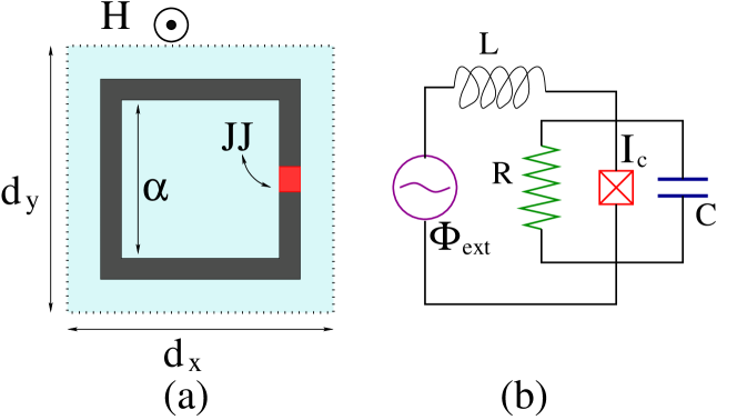
Figure 1: (color online) (a) Schematic drawing of an rf SQUID in a perpendicular time-dependent magnetic field ${\bf H}(t)$. (b) Equivalent electrical circuit ($RCSJ$ model) for a single rf SQUID driven by a flux source $\Phi_{ext}$.

Moreover, at low (sub-Kelvin) temperatures provide access to the quantum regime, where rf SQUIDs can be manipulated as flux and phase qubits Poletto2009 ; Castellano2010 , the basis element for quantum computation. Inductively coupled SQUID flux qubits can be used for the realization of quantum gates Zhou2005 , while larger arrays of inductively coupled SQUID flux qubits have been proposed as scalable systems for adiabatic quantum computing Roscilde2005 ; Johnson2010 . Notably, amplification and squeezing of quantum noise has been recently achieved with a tunable SQUID-based metamaterial Castellanos2008 .

In the present work we investigate the response of a two-dimensional (2D) rf SQUID metamaterial in the planar geometry with respect to frequency variation of an alternating magnetic field, focusing on the effect of quenched disorder through the SQUID parameter $\beta$ that determines the resonance frequency of individual SQUIDs. We are particularly interested in frequencies near resonance where multiple responses may appear; this issue is related to the existence or not of a bistability region in the current-frequency curve of the SQUID metamaterial. Having calculated the response of the metamaterial to a given alternating filed, the effective magnetic permeability $\mu_{r}$ can be determined by temporal and spatial averaging. Different responses, corresponding to different simultaneously stable metamaterial states, result in different $\mu_{r}$ in the bistability region. In the next section we give a brief overview of the equations for a single SQUID, we introduce the equations for the flux dynamics in a 2D SQUID metamaterial and calculate its linear modes. In Section 3 we present numerical results for the maximum total current (devided by the total number of SQUIDs) as a function of the driving frequency. Such current-frequency curves are obtained both for ordered and disordered SQUID metamaterials, focusing primarily on the possibility of bistability. In Section 4 we discuss the effect of synchronization and present calculations of the relative magnetic permeability $\mu_{r}$. Section 5 contains the conclusions.

II Dynamic Equations and Linear Modes

In an ideal JJ, the current-phase relation is of the form $I=I_{c}\,\sin(\phi_{j})$, where $I_{c}$ is the critical current of the JJ and $\phi_{j}$ the Josephson phase. When driven by an external magnetic field $H(t)$, the induced (super)currents around the SQUID ring are determined by the celebrated Josephson relations Josephson1962 . In the equivalent circuit picture, the resistively and capacitively shunted junction (RCSJ) model is frequently adopted to describe a real JJ. Thus, the equivalent lumped circuit for the rf SQUID in a magnetic field with appropriate polarization comprises a flux source $\Phi_{ext}$ in series with an inductance $L$ and an ideal JJ, while the latter is shunted by a capacitor $C$ and a resistor $R$ [figure 1(b)]. Then, the dynamic equation for the flux threading the SQUID ring can be obtained by application of Kirkhhoff laws, as

$$C\frac{d^{2}\Phi}{dt^{2}}+\frac{1}{R}\frac{d\Phi}{dt}+I_{c}\,\sin\left(2\pi\frac{\Phi}{\Phi_{0}}\right)+\frac{\Phi-\Phi_{ext}}{L}=0,$$ (1)

where $\Phi_{ext}$ is the external flux, $\Phi_{0}$ is the magnetic flux quantum, and $t$ is the temporal variable. The flux $\Phi$ threading the SQUID ring is related to the Josephson phase through the flux quantization condition

$$\phi_{j}=2\pi\frac{\Phi}{\Phi_{0}}+2\pi n,$$ (2)

where $n$ can be any integer.

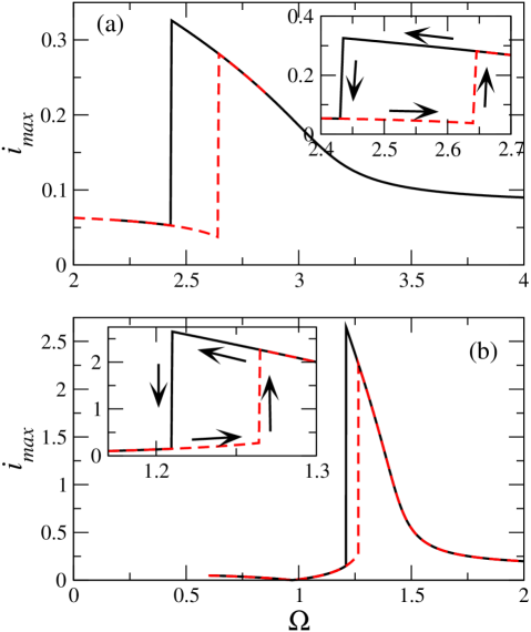
Figure 2: (color online) Maximum current amplitude $i_{max}$ as a function of the driving frequency $\Omega$ for an rf SQUID with $\alpha=0.002$, $\phi_{dc}=0$, and (a) $\beta=1.27$, $\phi_{ac}=0.1$; (b) $\beta=0.15$, $\phi_{ac}=0.02$. An enlargement of the bistability region is shown in the insets for each case.

The rf SQUID is a highly nonlinear oscillator whose amplitude-frequency curves exhibit several peculiar features not seen in conventional inductive-capacitive oscillators. For example, in a fine scale one may observe internal structure of increasing complexity that increases with increasing $\beta$ Shnyrkov1980 . That fine structure of the amplitude-frequency curves can be reproduced numerically by integrating the dynamic equation (1) Lazarides2008 ; Lazarides2012 . The SQUID resonance can be tuned either by varying the amplitude of the alternating driving field or by varying the magnitude of a static (dc) field threading the SQUID ring that creates a flux bias. The resonance shift due to nonlinearity has been actually observed in a Josephson parametric amplifier driven by fields of different power levels Castellanos2007 , while the shift with applied DC flux has been seen in high$-T_{c}$ rf SQUIDs Zeng2000 and very recently in a low$-T_{c}$ rf SQUID in the linear regime Jung2013 . Systematic measurements on microwave resonators comprising SQUID arrays are presented in references Castellanos2007 ; Palacios2008 . For very low amplitude of the driving field (linear regime), the rf SQUID exhibits a resonant magnetic response at a particular frequency $\omega_{SQ}=\omega_{0}\sqrt{1+\beta_{L}}$, where $\omega_{0}=1/\sqrt{LC}$ is the inductive-capacitive SQUID frequency, and $\beta_{L}$ is the SQUID parameter

$$\beta_{L}=2\pi\beta=2\pi\frac{LI_{c}}{\Phi_{0}}.$$ (3)

The dynamic behavior of the rf SQUID has been studied extensively for more than two decades both in the hysteretic ($\beta_{L}>1$) and the non-hysteretic regimes, usually under an external flux field of the form

$$\Phi_{ext}=\Phi_{dc}+\Phi_{ac}\cos(\omega t),$$ (4)

where $\omega$ is the driving frequency. The first and second term on the right-hand-side of the earlier equation correspond to the fluxes due to the presence of a constant (dc) and an alternating (ac) spatially uniform magnetic field, respectively. Typical current amplitude-frequency curves for a single SQUID are shown in figure 2 (for $\Phi_{dc}=0$). Equation (1) is formally equivalent to that of a massive particle in a tilted washboard potential (figure 3)

$$U_{SQ}=\frac{1}{C}\left\{\frac{(\Phi-\Phi_{ext})^{2}}{2L}-E_{j}\,\cos\left(2\pi\frac{\Phi}{\Phi_{0}}\right)\right\},$$ (5)

with $E_{j}=I_{c}\Phi_{0}/(2\pi)$ being the Josephson energy. While for $\beta_{L}<1$ there the potential has a single minimum, it aquires more and more local minima as $\beta_{L}$ increases above unity. Moreover, applied dc flux moves the location of both the local and the global minima.

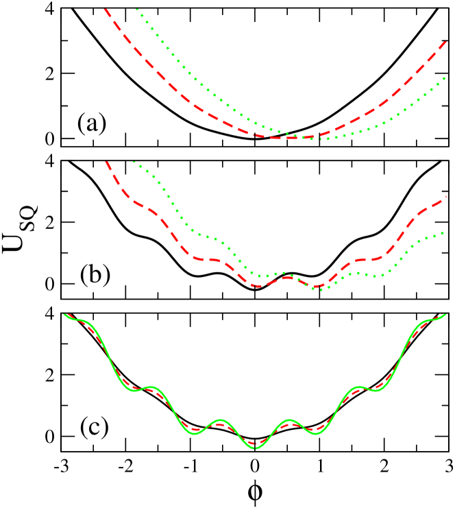
Figure 3: (color online) Potential curves as a function of the flux threading the SQUID ring. (a) For a non-hysteretic SQUID with $\beta_{L}\simeq 0.75<1$ and $\phi_{dc}=\Phi_{dc}/\Phi_{0}=0$ (black-solid curve); $0.5$ (red-dashed curve); $1.0$ (green-dotted curve). (b) For a hysteretic SQUID with $\beta_{L}\simeq 8>1$ and $\phi_{dc}=\Phi_{dc}/\Phi_{0}=0$ (black-solid curve); $0.5$ (red-dashed curve); $1.0$ (green-dotted curve). (c) For $\Phi_{dc}=0$ and $\beta_{L}=0.5<1$ (black-solid curve); $1.5$ (red-dashed curve); $2.5$ (green-dotted curve).

Consider a planar array comprising identical rf SQUIDs arranged in a tetragonal $N_{x}\times N_{y}$ lattice, that is placed in a spatially uniform, alternating magnetic field directed perpendicularly to the plane of the SQUIDs. The flux threading each SQUID ring induces a current with both normal and superconducting components that generates its own magnetic field. The induced fields couple the SQUIDs to each other through magnetic dipole-dipole interactions. The strength of this magnetoinductive coupling falls off approximatelly as the inverse-cube of the distance between SQUIDs. If the distance between neighboring SQUIDs is such that they are weakly coupled, then next-nearest and more distant neighbor coupling can be neglected. In that case, we need to take into account nearest-neighbor interaction only between SQUIDs, and the flux threading $(n,m)-$th SQUID of the array is given by

$$\Phi_{n,m}=\Phi_{ext}+L\,\left[I_{n,m}+\lambda_{x}(I_{n-1,m}+I_{n+1,m})\right.$$

$$\left.+\lambda_{y}(I_{n,m-1}+I_{n,m+1})\right],$$ (6)

where $n=1,...,N_{x},\,m=1,...,N_{y}$, $I_{n,m}$ is the total current induced in the $(n,m)-$th SQUID, and $\lambda_{x,y}\equiv M_{x,y}/L$ are the magnetic coupling constants between neighboring SQUIDs in the $x$ and $y$ directions, respectively. The values of the $M_{x}$ and $M_{y}$ are negative since the magnetic field generated by the induced current in a SQUID crosses the neighboring SQUID in the opposite direction. By adopting the resistively and capacitively shunted junction (RCSJ) model, the current $I_{n,m}$ is

$$-I_{n,m}=C\frac{d^{2}\Phi_{n,m}}{dt^{2}}+\frac{1}{R}\frac{d\Phi_{n,m}}{dt}+I_{c}\,\sin\left(2\pi\frac{\Phi_{n,m}}{\Phi_{0}}\right).$$ (7)

Then, following the procedure of reference Lazarides2008 and neglecting terms of order $\lambda_{x}\lambda_{y}$, $\lambda_{y}^{2}$, $\lambda_{x}^{2}$, etc., we get

$$C\frac{d^{2}\Phi_{n,m}}{dt^{2}}+\frac{1}{R}\frac{d\Phi_{n,m}}{dt}+I_{c}\,\sin\left(2\pi\frac{\Phi_{n,m}}{\Phi_{0}}\right)$$

$$-\lambda_{x}(\Phi_{n-1,m}+\Phi_{n+1,m})-\lambda_{y}(\Phi_{n,m-1}+\Phi_{n,m+1})$$

$$=[1-2(\lambda_{x}+\lambda_{y})]\Phi_{ext}.$$ (8)

In the absence of losses ($\gamma=0$), the earlier equations can be obtained from the Hamiltonian function

$$H=\sum_{n,m}\frac{Q_{n,m}^{2}}{2C}$$

$$+\sum_{n,m}\left[\frac{1}{2L}(\Phi_{n,m}-\Phi_{ext})^{2}-E_{J}\,\cos\left(2\pi\frac{\Phi_{n,m}}{\Phi_{0}}\right)\right]$$

$$-\sum_{n,m}\frac{\lambda_{x}}{L}(\Phi_{n,m}-\Phi_{ext})(\Phi_{n-1,m}-\Phi_{ext})$$

$$-\sum_{n,m}\frac{\lambda_{y}}{L}(\Phi_{n,m}-\Phi_{ext})(\Phi_{n,m-1}-\Phi_{ext}),$$ (9)

and

$$Q_{n,m}=C\,\frac{d\Phi_{n,m}}{dt}$$ (10)

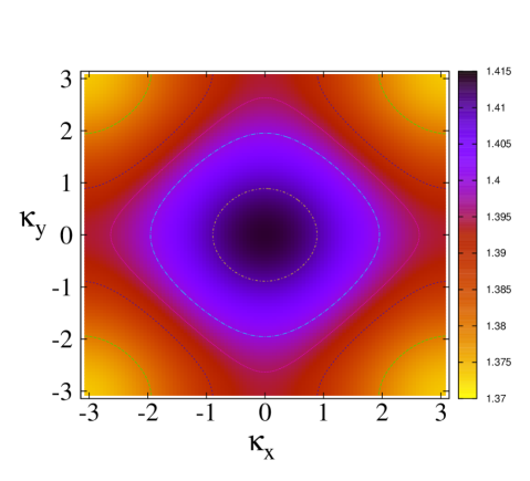
Figure 4: (color online) Contours of the linear dispersion $\Omega_{\vec{\kappa}}$ on the $\kappa_{x}-\kappa_{y}$ plane for a two-dimensional rf SQUID array, with $\lambda_{x}=\lambda_{y}=-0.014$ and $\beta=0.15$.

is the canonical variable conjugate to $\Phi_{n,m}$, and represents the charge accumulating across the capacitance of the JJ of each rf SQUID. The Hamiltonian function (II) is the weak coupling version of that proposed in the context of quantum computation Roscilde2005 . Using the relations

$$\phi_{n,m}=\frac{\Phi_{n,m}}{\Phi_{0}},\phi_{ext}=\frac{\Phi_{ext}}{\Phi_{0}},\tau=\omega_{0}t,\Omega=\frac{\omega}{\omega_{0}},$$ (11)

and equations (3), (14), equations (II) are normalized to

$$\ddot{\phi}_{n,m}+\gamma\dot{\phi}_{n,m}+\phi_{n,m}+\beta\,\sin(2\pi\phi_{n,m})$$

$$-\lambda_{x}(\phi_{n-1,m}+\phi_{n+1,m})-\lambda_{y}(\phi_{n,m-1}+\phi_{n,m+1})$$

$$=\phi_{eff},$$ (12)

where the overdots denote differentiation with respect to the normalized time $\tau$,

$$\phi_{eff}=[1-2(\lambda_{x}+\lambda_{y})]\phi_{ext},$$ (13)

is the effective driving field, and

$$\gamma=\frac{1}{R}\sqrt{\frac{L}{C}},$$ (14)

is the loss coefficient of individual SQUIDs, that actually represents all of the dissipation coupled to each rf SQUID and may also include radiative losses Kourakis2007 .

SQUID metamaterials support magnetoinductive flux-waves Lazarides2008 , just like conventional metamaterials comprising metallic elements (i.e., split-ring resonators) Shamonina2002 . The frequency dispersion for small amplitude flux waves is obtained by the substitution of $\phi=A\,\exp[i(\kappa_{x}n+\kappa_{y}m-\Omega\tau)]$, into the linearized equation (11) without losses and external field ($\gamma=0$, $\phi_{ext}=0$)

$$\Omega=\sqrt{1+\beta_{L}-2(\lambda_{x}\,\cos\kappa_{x}+\lambda_{y}\,\cos\kappa_{y})},$$ (15)

where $\Omega=\omega/\omega_{0}$ and $\kappa_{x,y}=d_{x,y}\,k_{x,y}$ are the normalized wavevector components, with $k_{x}$ ($k_{y}$) and $d_{x}$ ($d_{y}$) being the wavevector component and center-to-center distance between neighboring SQUIDs in $x-$direction ($y-$direction), respectively.

III Current - Frequency Curves

In the following, equations (II) are implemented with the boundary condition (except otherwise stated)

$$\phi_{0,m}(\tau)=\phi_{N_{x}+1,m}(\tau)=\phi_{n,0}(\tau)=\phi_{n,N_{y}+1}(\tau)=0,$$ (16)

for $n=1,...,N_{x}$, $m=1,...,N_{y}$ that account for the termination of the structure in a finite system. The set of dynamic equations (16) are integrated in time with a standard 4th order Runge-Kutta algorithm. For a single SQUID, the current denoted by $i_{max}$ is just the amplitude of the induced current. In the case of ordered SQUID arrays we use the same notation for the maximum total current, i.e., $i_{max}=max\left\{\frac{1}{N_{x}N_{y}}\sum_{n,m}i_{n,m}(t)\right\}$, where $n=1,...,N_{x}$ and $m=1,...,N_{y}$. For disordered arrays, the brackets $<...>$ indicate averaging of the maximum total current of the array over the number of differnt realizations, $n_{r}$. In order to trace the current-frequency curves for ordered ($i_{max}-\Omega$) or disordered ($<i_{max}>-\Omega$) arrays, we start the system with zero initial conditions and start integrating with a low (high) frequency until a steady state is reached. Subsequently the frequency is increased (decreased) by a small amount and the equations are again integrated until a steady state is reached, and so on. In each frequency step (except the first one, where we use zeros) we use as initial condition the steady state solution obtained in the previous step.

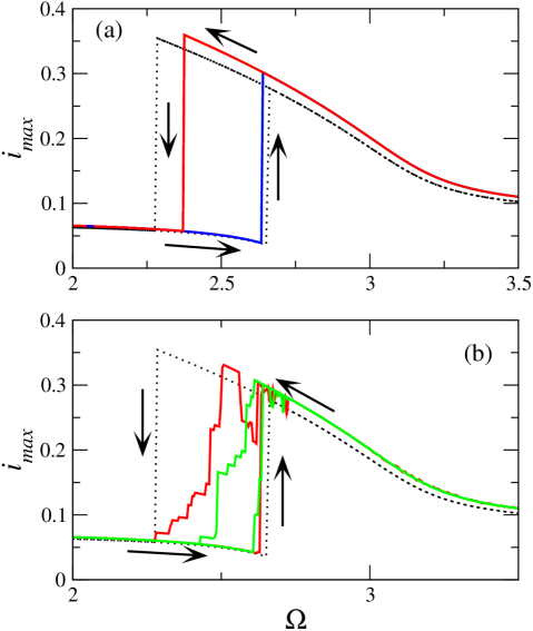
Figure 5: (color online) Maximum total current amplitude $i_{max}$ as a function of the driving frequency $\Omega$ for two-dimensional $N_{x}\times N_{y}$ rf SQUID arrays with $\alpha=0.002$, $\beta=1.27$, $\phi_{dc}=0$, $\phi_{ac}=0.1$, $N_{x}=N_{y}=20$, and (a) periodic boundary conditions; (b) free-end boundary conditions, starting with different initializations. The black dotted lines indicate the corresponding $i_{max}$ vs. $\Omega$ curves for a single rf SQUID. The maximum total current of the arrays has been divided by the total number of rf SQUIDs $N_{x}\times N_{y}$ to facilitate the comparison.

The bistability properties of single SQUID oscillators (see figure 2) are also seen in the arrays as well. We assume a moderate size array with $N_{x}=N_{y}=20$, for which the coupling between SQUIDs is isotropic and weak, i.e., $\lambda_{x}=\lambda_{y}=-0.014$. Typical current-frequency curves are shown in figure 5, where the maximum of the total current, divided by the total number of SQUIDs in the array, is displayed as function of the frequency $\Omega$ of an alternating flux (dc flux is set to zero). In this figure, the value of $\beta-$parameter has been selected so that hysteretic effects are rather strong ($\beta_{L}\simeq 8$). We observe that bistability appears in a frequency region of significant width. The corresponding curves for a single SQUID are also shown for comparison. In figure 5(a), where periodic boundary conditions have been employed, we observe that although the bistability region for the array is narrower than that for a single SQUID, the maximum current per SQUID is slightly larger than that for a single SQUID. In the case of periodic boundary conditions, the size of the array does not affect those results; current-frequency curves for larger arrays with $N_{x}=N_{y}=40$ and $N_{x}=N_{y}=80$ (not shown) are practically identical to these shown in figure 5(a). In figure 5(b) and the rest of the paper free-end boundary conditions [equations (16)] have been used. In this case, the current-frequency curves are very sensitive to the initial conditions, the frequency step, and other parameters. The curves in figure 5(b) shown in different colours (red and green) correspond to different initializations of the same system.

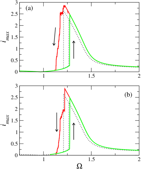
Figure 6: (color online) Maximum total current amplitude $i_{max}$ as a function of the driving frequency $\Omega$ for two-dimensional $N_{x}\times N_{y}$ rf SQUID arrays with $\alpha=0.002$, $\beta=0.15$, $\phi_{dc}=0$, $\phi_{ac}=0.02$, and (a) $N_{x}=N_{y}=20$; (b) $N_{x}=N_{y}=40$. The black dotted lines indicate the corresponding $i_{max}$ vs. $\Omega$ curves for a single rf SQUID. The maximum total current of the arrays has been divided by the total number of rf SQUIDs $N_{x}\times N_{y}$ to facilitate the comparison. Free-end boundary conditions that account for the termination of the structure have been used.

The parts of current-frequency curves that are close to those for the single SQUID are formed by almost homogeneous states, i.e., states with all SQUIDs in the high-current or low-current state. Homogeneous states are formed easier in the periodic systems [figure 5(a)]; only a small part survives in the case of free boundary conditions [figure 5(b)] that is close to the current-frequency curve of the single SQUID. In the latter figure we also observe the formation of small steps for which the corresponding solutions may be characterized as ’mixed states’, that are formed by a certain number of SQUIDs in the high-current state while all the others are in the low-current state. In figure 6, the corresponding curves for SQUIDs with $\beta_{L}\simeq 1$ ($\beta=0.15$) are shown. A comparison with the corresponding curves for a single SQUID (shown as dotted black lines) indicates that the frequency region where bistability appears are nearly of the same width.

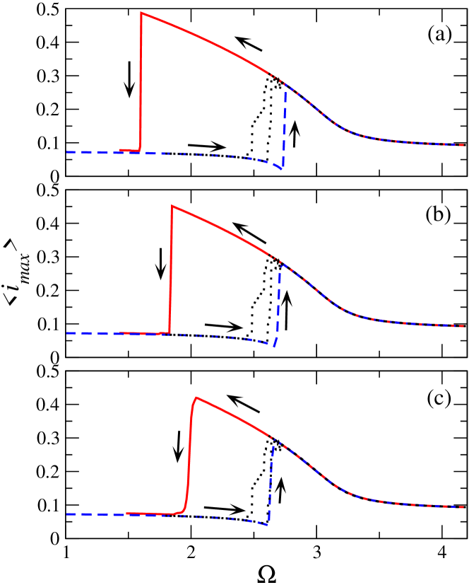
Figure 7: (color online) Maximum current amplitude averaged over $N_{R}=30$ realizations od disorder, $<i_{max}>$, as a function of the driving frequency $\Omega$ for a SQUID metamaterial with $\alpha=0.002$, $\beta=1.27$, $\phi_{ac}=0.1$, $\phi_{dc}=0$, and (a) $\beta=1.27~{}\pm 0.01$; (b) $\beta=1.27~{}\pm 0.05$; (c) $\beta=1.27~{}\pm 0.1$. The corresponding curves for the same SQUID metamaterial without disorder are shown in black-dotted lines.

The assumption of SQUID-based metamaterials comprising identical elements is certainly not realistic. Therefore, we consider disordered SQUID arrays in which the parameter $\beta$ varies randomly within a particular range of values around a mean value. The SQUID parameter $\beta$, that depends on the critical current of the Josephson junctions, determines also the resonance frequency of individual SQUIDs. We have calculated the maximum current-frequency curves of the same SQUID metamaterials as before, taking into account the distribution of the natural frequencies of individual SQUIDs. For obtaining reliable results, we have taken statistical averages over many realizations, $n_{R}$, of disorder. Remarkably, the calculations reveal that weak disorder strongly favours bistability, as it is observed in figures 7 and 8 for mean values of $\beta=1.27$ and $0.15$, respectively. In these figures, as we go from (a) to (c) $\beta$ fluctuates by $\pm 0.01$, $\pm 0.05$, and $\pm 0.1$, so that the relative disorder strength is much larger in figure 8. In all cases shown, either exhibiting weak or strong disorder, the stability of the nearly homogeneous states with high current increases considerably with respect to that for the corresponding ordered SQUID metamaterials. This is actually reflected in the widening of the bistability regions of the current frequency curves. We should also note that the bistability region gradually shrinks with increasing strength of disorder. That shrinking occurs more rapidly for $\beta_{L}\simeq 1$ (figure 8) since the relative $\beta$ variation is larger in this case.

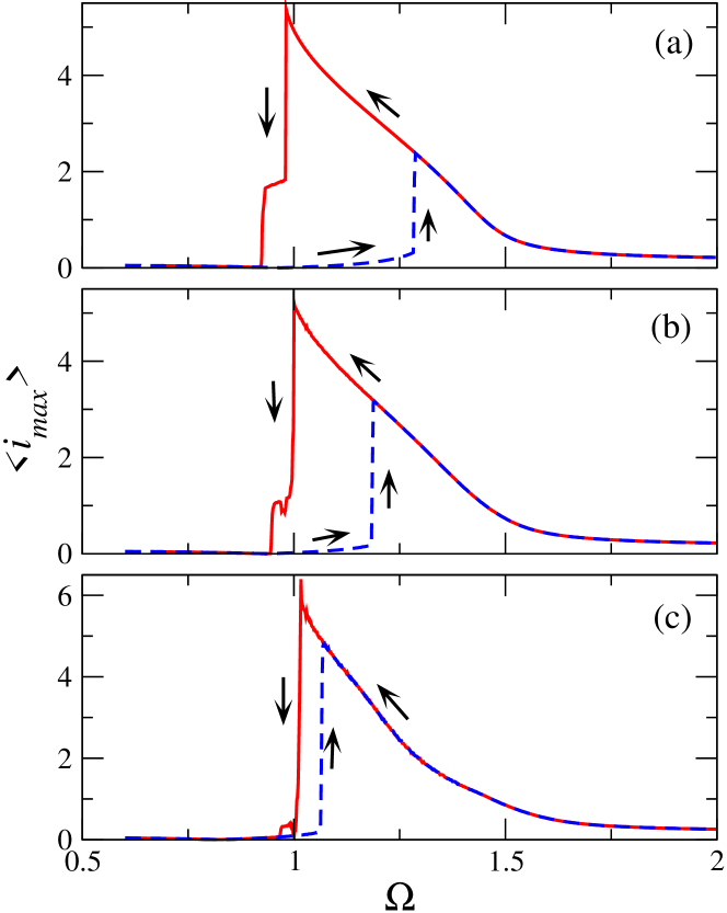
Figure 8: (color online) Maximum current amplitude averaged over $N_{R}=30$ realizations od disorder, $<i_{max}>$, as a function of the driving frequency $\Omega$ for a SQUID metamaterial with $\alpha=0.002$, $\beta=0.15$, $\phi_{ac}=0.02$, $\phi_{dc}=0$, and (a) $\beta=1.27~{}\pm 0.01$; (b) $\beta=1.27~{}\pm 0.05$; (c) $\beta=1.27~{}\pm 0.1$. The corresponding curves for the same SQUID metamaterial without disorder are shown in black-dotted lines.

IV Synchronization and Multiresponse

In order to ensure that the maximum current-frequency curves presented in figures 7 and 8 correspond to homogeneous states, we define and calculate a (Kuramoto-type) synchronization parameter, as

$$\Psi=\left<\frac{1}{N_{x}\,N_{y}}\sum_{n,m}e^{2\pi i\phi_{n,m}}\right>_{\tau,n_{R}},$$ (17)

where the brackets denote averaging both in time (i.e., in one oscillation period) and the number of realizations of disorder $n_{R}$. The absolute value of $\Psi$ quantifies the degree of synchronization; $|\Psi|$ may vary between $0$ and $1$, corresponding to completely asynchronous and synchronized states, respectively. The calculated values for (parts of) the maximum current-frequency curves in figure 7 are shown in figure 9 for $\Omega$ varying in both directions. The bistability regions are shown in this figure as green-dotted vertical lines, for reference. For very weak disorder [figure 9(a)], $|\Psi|$ remains close to unity for most of the frequency interval shown. However, there is a narrow region at low frequencies where synchronization, and therefore complete homogeneity breaks down, when the high current solution loses its stability. In that case all the SQUIDs change their state towards a lower maximum current state. During the proccess, the phase differences of the SQUID fluxes and the driving field lock in randomly selected values, resulting in a low current and only partially synchronized state. However, the two low current states that can be distinguish in this frequency region, i.e., the synchronized one obtained with increasing frequency and the partially synchronized one obtained with decreasing frequency, provide almost the same maximum current. With increasing the strength of the disorder [figure 9(b)] the bistability region shinks while the same effect as in figure 9(a) is observed in a wider frequency interval. Moreover, the high current states are not completely synchronized in the bistability region, since $|\Psi|$ is slightly less than unity. The effect can be seen more clearly by further increasing the strength of the disorder as in figure 9(c), where $|\Psi|$ is clearly less than unity in the bistability region indicating partial synchronization.

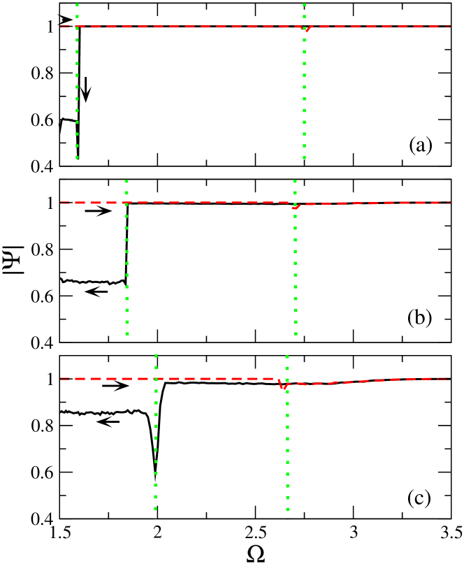
Figure 9: (color online) The magnitude of the synchronization parameter $|\Psi|$ as a function of the driving frequency $\Omega$ in the bistability region, for a $N_{x}\times N_{y}=20\times 20$ SQUID metamaterial with $\alpha=0.002$, $\beta=1.27\pm 0.01$, $\phi_{ac}=0.1$, $\phi_{dc}=0$, $N_{R}=30$ realizations of disorder, and (a) $\beta=1.27\pm 0.01$; (b) $\beta=1.27\pm 0.05$; $\beta=1.27\pm 0.1$. The arrows indicate the direction of frequency variation while the green dotted lines the corresponding bistability intervals.

The magnetic response of the SQUID metamaterial at a particular state can be calculated in terms of the magnetization along the lines given in references Lazarides2007 ; Jung2013 . Assuming a tetragonal unit cell with $d_{x}=d_{y}=d$ and a squared SQUID area of side $\alpha$, the magnetization is

$$M=\frac{\alpha^{2}<I>}{d^{2}D},$$ (18)

where $<I>=I_{c}\,<i>\equiv I_{c}\frac{1}{N_{x}N_{y}}\sum_{n,m}<i_{n,m}>_{\tau}$ is the spatially and temporally averaged current, and $D$ is a length related to the cavity where the metamaterial is placed Jung2013 . Using fundamental relations of electromagnetism we write the relative magnetic permeability as

$$\mu_{r}=1+\frac{M}{H},$$ (19)

where $H$ is the intensity of a spatially uniform magnetic field applied perpendicularly to the SQUID metamaterial plane. The latter is related to the external flux to the SQUIDs as

$$H=\frac{\Phi_{0}}{\mu_{0}\alpha^{2}}<\phi_{ext}>,$$ (20)

where $\mu_{0}$ is the magnetic permeability of the vacuum, and the brackets denote temporal averaging. Combining equations (18)-(20), we get

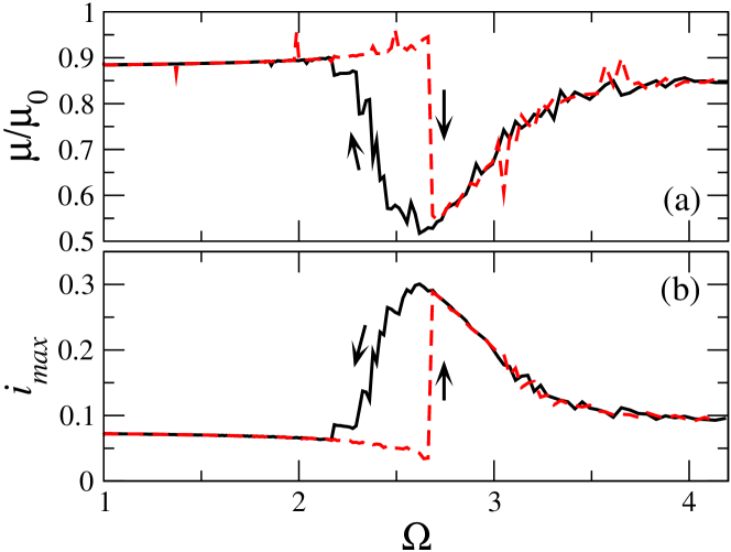
Figure 10: (color online) (a) Relative magnetic permeability $\mu_{r}=\mu/\mu_{0}$ for the low and high maximum current states as a function of the driving frequency $\Omega$, for $N_{x}=N_{y}=20$, $\alpha=0.002$, $\beta=1.27$, $\phi_{ac}=0.1$, and $\phi_{dc}=0$. Multiple-valued magnetic response is observed in the bistability region. (b) The corresponding maximum current-frequency curves. The arrows indicate the direction of frequency variation.

$$\mu_{r}=1+\kappa\frac{<i>}{<\phi_{ext}>},$$ (21)

where $\kappa=\frac{\mu_{0}\alpha I_{c}}{\Phi_{0}}\frac{\alpha^{3}}{d^{2}D}$. For a rough estimation of the constant $\kappa$ assume that $L\sim\mu_{0}\alpha$, where $L$ is the SQUID inductance, and that $D\simeq d$. Then, we have that $\kappa\sim\beta\left(\frac{\alpha}{d}\right)^{3}$. Using $\alpha=d/2$ and $\beta=1.27$ we get $\kappa\simeq 0.16$. We may then use the numerically calculated values of $i_{n,m}$ and $\phi_{ext}$ into equation (21) to obtain $\mu_{r}$. Simultaneously stable SQUID metamaterial states respond differently to the external field and therefore exhibit different $\mu_{r}$. This can be seen clearly in figure 10, where the relative permeability $\mu_{r}$ has been calculated from equation (21). The SQUID metamaterial for the parameters used in figure 10 is diamagnetic for all frequencies; however, the diamagnetic response is stronger for the high current states in the bistability region. For a weaker driving field that provides a flux amplitude of $10^{-3}$ the metamaterial is in the linear limit, as can be infered by inspection of the current-frequency curve shown in figure 11(b). The corresponding $\mu_{r}$ as a function of the driving frequency $\Omega$ is again diamagnetic everywhere except close to the resonance, where strong variation of $\mu_{r}$ occurs. For frequencies below (but very close to) the resonance at $\Omega\sim 3$ the metamaterial becomes strongly paramagnetic. To the contrary, for frequencies above (but very close to) the resonance the metamaterial becomes extremely diamagnetic, exhibiting negative $\mu_{r}$ within a narrow frequency region. Note that in this case negative $\mu_{r}$ would have also been obtained with a much smaller coefficient $\kappa$.

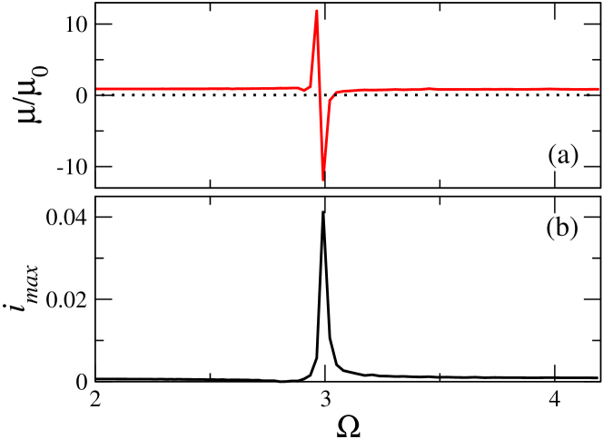
Figure 11: (color online) (a) Relative magnetic permeability $\mu_{r}=\mu/\mu_{0}$ for the low and high maximum current states as a function of the driving frequency $\Omega$, for $N_{x}=N_{y}=20$, $\alpha=0.002$, $\beta=1.27$, $\phi_{ac}=0.001$, and $\phi_{dc}=0$. Negative $\mu_{r}$ is observed in a narrow frequency band just above the resonance frequency. (b) The corresponding maximum current-frequency curves.

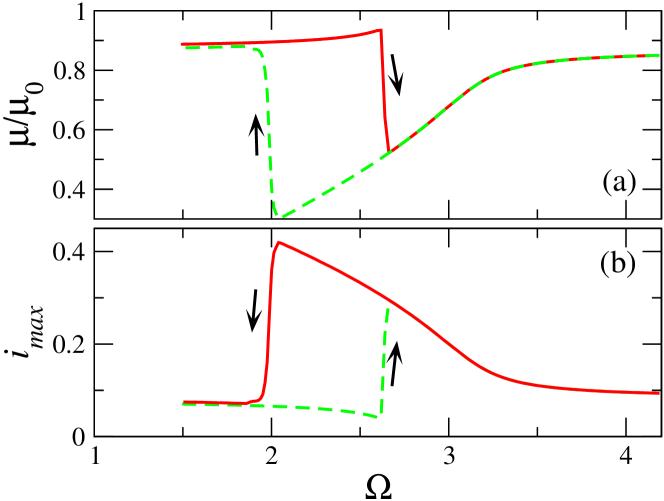
Figure 12: (color online) (a) Relative magnetic permeability $\mu_{r}=\mu/\mu_{0}$ for the low and high maximum current states as a function of the driving frequency $\Omega$, for a disordered SQUID metamaterial, with $N_{x}=N_{y}=20$, $\alpha=0.002$, $\beta=1.27\pm 0.1$, $\phi_{ac}=0.1$, and $\phi_{dc}=0$. Multiple-valued magnetic response is observed in the bistability region. (b) The corresponding maximum current-frequency curves.

For a disordered SQUID metamaterial, that is relatively strongly driven ($\phi_{ac}=0.1$), the relative permeability $\mu_{r}$ changes only slightly. The most important effect observed in this case is the enlargement of the bistability interval (figure 12). For weakly driven, disordered SQUID metamaterial, increasing disorder results in decreasing of the magnitude of $\mu_{r}$ in the frequency region around resonance. This effect is illustrated in figures 13 and 14, obtained for two different values of disorder; $\beta$ fluctuates around its mean value by $\pm 0.01$ and $\pm 0.1$, respectively. In the frequency region around resonance, in particular, we observe in figure 13 that the dip corresponding to negative $\mu_{r}$ becomes shallower than that for the ordered SQUID metamaterial (figure 11). With further increasing disorder (figure 14), the negative $\mu_{r}$ region disappears. For this particular set of parameters, the minimum of $\mu_{r}$ touches the zero axis.

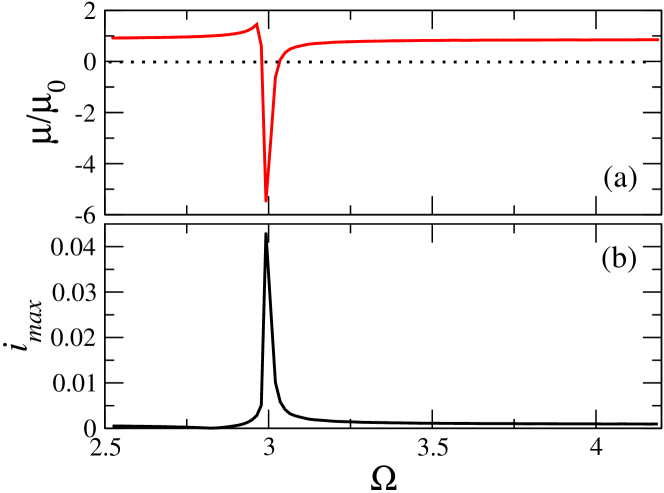
Figure 13: (color online) (a) Relative magnetic permeability $\mu_{r}=\mu/\mu_{0}$ for the low and high maximum current states as a function of the driving frequency $\Omega$, for a disordered SQUID metamaterial, with $N_{x}=N_{y}=20$, $\alpha=0.002$, $\beta=1.27\pm 0.01$, $\phi_{ac}=0.001$, and $\phi_{dc}=0$. Negative $\mu_{r}$ is observed in a narrow frequency band just above the resonance frequency. (b) The corresponding maximum current-frequency curves.

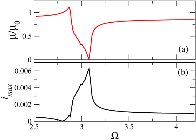
Figure 14: (color online) (a) Relative magnetic permeability $\mu_{r}=\mu/\mu_{0}$ for the low and high maximum current states as a function of the driving frequency $\Omega$, for a disordered SQUID metamaterial, with $N_{x}=N_{y}=20$, $\alpha=0.002$, $\beta=1.27\pm 0.1$, $\phi_{ac}=0.001$, and $\phi_{dc}=0$. Negative $\mu_{r}$ is not observed because of the relatively stong disorder. (b) The corresponding maximum current-frequency curves.

V Conclusions.

We investigated numerically two-dimensional SQUID metamaterials driven by an alternating magnetic field. We have calculated current-frequency curves both for ordered and disordered metamaterials; in both cases we observed bistability regions created by almost homogeneous high and low current states. However, we observed that the presence of disorder widens significantly the bistability regions. The effect is rather strong for SQUID metamaterials comprising SQUIDs with either small or large $\beta_{L}$ parameter. Remarkably, the homogeneity of high and low current states, that is quantified by the parameter $\Psi$, persists also in the case of disorder up to a very high degree. These states deviate only slightly from practically complete homogeneity only in the case of strong disorder, as can be seen from calculations of the amplitude of $\Psi$. This important result indicates that random variation of the SQUID parameters does not destroy bistability, that is crusial for applications that require bistable switching properties, but instead stabilizes the system against modulational or other instabilities.

This result is related to past work on disordered networks of nonlinear oscillators where it was concluded that moderate disorder may enhance synchronization and stabilize the system against chaos Braiman1995a ; Braiman1995b . In the present context, synchronization of individual SQUIDs in the high or low current states results in high or low maximum total current for the metamaterial. This requires that (almost) all the SQUIDs are in phase. It could be natural to assume that the more nearly identical the elements, the better the synchronization will be. However, even in the ideal case of identical elements, the earlier assumption may not be true and the in phase state may be dynamically unstable. Then, synchronization is reduced and the SQUID metamaterial cannot remain in the high current state that is more sensitive to instability. This can be clearly observed in figures 5(b) and 6(b), where in most of the bistability region the metamaterial relaxes to partially synchronized states that provide significantly lower maximum total current. This type of disorder-assisted self-organization may also occur by introducing local disorder in an array of otherwise identical oscillators, i.e., in the form of impurities Gavrielides1998a ; Gavrielides1998b . In this case, the impurities trigger a self-organizing process that brings the system to complete synchronization and suppression of chaotic behaviour.

Having calculated numerically the response of the metamaterial to an alternating field with given frequency, we have calculated the magnetic permeability of the metamaterial for several illustrating cases both with and without disorder. While the expression for calculating the magnetic permeability is rather simple, there is some uncertainty about the value of the factor $\kappa$. However, for a reasonable value of $\kappa$ we observe that the magnetic permeability can take negative values in a narrow frequency region above resonance for weakly driven SQUID metamaterials. In this case, increasing disorder results in weakening the negative response of the metamaterial; thus, for relatively strong disorder the response is not sufficient to make the magnetic permeability negative. For SQUID metamaterials exhibiting bistability, different magnetic permeabilities can be reached under the same conditions depending on their state.

References

- (1) V.M. Shalaev, Nature Photonics 1, 41 (2007)
- (2) C.M. Soukoulis, S. Linden, M. Wegener, Science 315, 47 (2007)
- (3) N.M. Litchinitser, V.M. Shalaev, Laser Phys. Lett. 5, 411 (2008)
- (4) N.I. Zheludev, Science 328, 582 (2010)
- (5) J.B. Pendry, Phys. Rev. Lett. 85, 3966–3969 (2000)
- (6) D. Schurig, J.J. Mock, B.J. Justice, S.A. Cummer, J.B. Pendry, A.F. Starr, D.R. Smith, Science 314, 977 (2006)
- (7) N.I. Zheludev, Optics and Photonics News 22, 31 (2011)
- (8) J.G. Caputo, I. Gabitov, A.I. Maimistov, Phys. Rev. B 85, 205446 (2012)
- (9) I.V. Shadrivov, A.B. Kozyrev, D.W. van der Weide, Y.S. Kivshar, Appl. Phys. Lett. 93, 161903 (2008)
- (10) A.D. Boardman, V.V. Grimalsky, Y.S. Kivshar, S.V. Koshevaya, M. Lapine, N.M. Litchinitser, V.N. Malnev, M. Noginov, Y.G. Rapoport, V.M. Shalaev, Laser Photonics Rev. 5 (2), 287 (2010)
- (11) S.M. Anlage, J. Opt. 13, 024001 (2011)
- (12) M.C. Ricci, N. Orloff, S.M. Anlage, Appl. Phys. Lett. 87, 034102 (3pp) (2005)
- (13) M.C. Ricci, H. Xu, R. Prozorov, A.P. Zhuravel, A.V. Ustinov, S.M. Anlage, IEEE Trans. Appl. Superconduct. 17, 918 (2007)
- (14) J. Gu, R. Singh, Z. Tian, W. Cao, Q. Xing, M.X. He, J.W. Zhang, J. Han, H. Chen, W. Zhang, Appl. Phys. Lett. 97, 071102 (3pp) (2010)
- (15) V.A. Fedotov, A. Tsiatmas, J.H. Shi, R. Buckingham, P. de Groot, Y. Chen, S. Wang, N.I. Zheludev, Opt. Express 18, 9015 (2010)
- (16) H.T. Chen, H. Yang, R. Singh, J.F. O’Hara, A.K. Azad, A. Stuart, S.A. Trugman, Q.X. Jia, A.J. Taylor, Phys. Rev. Lett. 105, 247402 (2010)
- (17) N. Lazarides, G.P. Tsironis, Appl. Phys. Lett. 16, 163501 (2007)
- (18) N. Lazarides, G.P. Tsironis, M. Eleftheriou, Nonlinear Phenomena in Complex Systems 11, 250 (2008)
- (19) A. Barone, G. Patternó., Physics and Applications of the Josephson Effect. (Wiley, New York, 1982)
- (20) K.K. Likharev., Dynamics of Josephson Junctions and Circuits. (Gordon and Breach, Philadelphia, 1986)
- (21) G.P. Tsironis, N. Lazarides, M. Eleftheriou, PIERS Online 5, 26 (2009)
- (22) N. Lazarides, G.P. Tsironis, Proc. SPIE 8423, 84231K (2012)
- (23) B. Josephson, Phys. Lett. A 1, 251 (1962)
- (24) P. Jung, S. Butz, S.V. Shitov, A.V. Ustinov, Appl. Phys. Lett. 102, 062601 (4pp) (2013)
- (25) R. Kleiner, D. Koelle, F. Ludwig, J. Clarke, Proceedings of the IEEE 92, 1534 (2004)
- (26) R.L. Fagaly, Review of Scientific Instruments 77, 101101 (2006)
- (27) W. Wernsdorfer, Supercond. Sci. Technol. 22, 064013 (2009)
- (28) J. Beyer, D. Drung, Supercond. Sci. Technol. 21, 095012 (6pp) (2008)
- (29) C. Häussler, T. Träuble, J. Oppenländer, N. Schopohl, IEEE Trans. Appl. Superconduct. 11, 1275 (2001)
- (30) A.C. Bruno, M.A. Espy, Supercond. Sci. Technol. 17, 908 (2004)
- (31) M. Matsuda, K. Nakamura, H. Mikami, S. Kuriki, IEEE Trans. Appl. Superconduct. 15, 817 (2005)
- (32) F. Hirayama, N. Kasai, M. Koyanagi, IEEE Trans. Appl. Superconduct. 9, 2923 (1999)
- (33) M.E. Huber, P.A. Neil, R.G. Benson, D.A. Burns, A.M. Corey, C.S. Flynn, Y. Kitaygorodskaya, O. Massihzadeh, J.M. Martinis, G.C. Hilton, IEEE Trans. Appl. Superconduct. 11, 1251 (2001)
- (34) M.A. Castellanos-Beltran, K.W. Lehnert, Appl. Phys. Lett. 91, 083509 (3pp) (2007)
- (35) V.K. Kaplunenko, J. Mygind, N.F. Pedersen, A.V. Ustinov, J. Appl. Phys. 73, 2019 (1993)
- (36) C. Häussler, J. Oppenländer, N. Schopohl, J. Appl. Phys. 89, 1875 (2001)
- (37) O. Brandel, O. Wetzstein, T. May, H. Toepfer, T. Ortlepp, H.G. Meyer, Supercond. Sci. Technol. 25, 125012 (6pp) (2012)
- (38) S. Poletto, F. Chiarello, M.G. Castellano, J. Lisenfeld, A. Lukashenko, P. Carelli, A.V. Ustinov, Physica Scripta T137, 014011 (6pp) (2009)
- (39) M.G. Castellano, F. Chiarello, P. Carelli, C. Cosmelli, F. Mattioli, G. Torrioli, New Journal of Physics 12, 043047 (13pp) (2010)
- (40) Z. Zhou, S.I. Chu, S. Han, IEEE Trans. Appl. Superconduct. 15, 833 (2005)
- (41) T. Roscilde, V. Corato, B. Ruggiero, P. Silvestrini, Phys. Lett. A 345, 224 (2005)
- (42) M.W. Johnson, P. Bunyk, F. Maibaum, E. Tolkacheva, A.J. Berkley, E.M. Chapple, R. Harris, J. Johansson, T. Lanting, I. Perminov, E. Ladizinsky, T. Oh, G. Rose1, Supercond. Sci. Technol. 23, 065004 (12pp) (2010)
- (43) M.A. Castellanos-Beltran, K.D. Irwin, G.C. Hilton, L.R. Vale, K.W. Lehnert, Nature Physics 4, 928 (2008)
- (44) V.I. Shnyrkov, V.A. Khlus, G.M. Choi, J. Low Temp. Phys. 39, 477 (1980)
- (45) X.H. Zeng, Y. Zhang, B. Chesca, K. Barthel, Y.S. Greenberg, A.I. Braginski, J. Appl. Phys. 88, 6781 (2000)
- (46) A. Palacios-Laloy, F. Nguyen, F. Mallet, P. Bertet, D. Vion, D. Esteve, J. Low Temp. Phys. 151, 1034 (2008)
- (47) I. Kourakis, N. Lazarides, G.P. Tsironis, Phys. Rev. E 75, 067601 (2007)
- (48) E. Shamonina, V.A. Kalinin, K.H. Ringhofer, L. Solymar, J. Appl. Phys. 92, 6252 (2002)
- (49) Y. Braiman, W.L. Ditto, K. Wiesenfeld, M.L. Spano, Phys. Lett. A 206, 54 (1995)
- (50) Y. Braiman, J.F. Lindner, W.L. Ditto, Nature 378, 465 (1995)
- (51) A. Gavrielides, T. Kottos, V. Kovanis, G.P. Tsironis, Europhys. Lett. 44, 559 (1998)
- (52) A. Gavrielides, T. Kottos, V. Kovanis, G.P. Tsironis, Phys. Rev. E 58, 5529 (1998)