Alternative Scenarios of Relativistic Heavy-Ion Collisions:
II. Particle Production

Abstract

Particle production in relativistic collisions of heavy nuclei is analyzed in a wide range of incident energies 2.7 GeV $\leq\sqrt{s_{NN}}\leq$ 62.4 GeV. The analysis is performed within the three-fluid model employing three different equations of state (EoS): a purely hadronic EoS, an EoS with the first-order phase transition and that with a smooth crossover transition. It is found that the hadronic scenario fails to reproduce experimental yields of antibaryons (strange and nonstrange), starting already from lower SPS energies, i.e. $\sqrt{s_{NN}}>$ 5 GeV. Moreover, at energies above the top SPS one, i.e. $\sqrt{s_{NN}}>$ 17.4 GeV, the mid-rapidity densities predicted by the hadronic scenario considerably exceed the available RHIC data on all species. At the same time the deconfinement-transition scenarios reasonably agree (to a various extent) with all the data. The present analysis demonstrates certain advantage of the deconfinement-transition EoS’s. However, all scenarios fail to reproduce the strangeness enhancement in the incident energy range near 30$A$ GeV (i.e. a horn anomaly in the $K^{+}/\pi^{+}$ ratio) and yields of $\phi$-mesons at 20$A$–40$A$ GeV.

I Introduction

This paper continues a series of reports on simulations of relativistic heavy-ion collisions within different scenarios Ivanov:2012bh ; 3FD-2012-stopping . These simulations were performed within a model of the three-fluid dynamics (3FD) 3FD employing three different equations of state (EoS): a purely hadronic EoS gasEOS (hadr. EoS), which was used in the major part of the 3FD simulations so far 3FD ; 3FD-GSI07 ; 3FDflow ; 3FDpt ; 3FDv2 , and two versions of EoS involving the deconfinement transition Toneev06 . These two versions are an EoS with the first-order phase transition and that with a smooth crossover transition. Details of these calculations are described in the first paper of this series 3FD-2012-stopping dedicated to analysis of the baryon stopping.

In this paper I report results on particle production and rapidity distributions of these particles in relativistic heavy-ion collisions in the energy range from 2.7 GeV to 62.4 GeV in terms of the center-of-mass incident energy ($\sqrt{s_{NN}}$). This domain covers the energy range of the RHIC (Relativistic Heavy-Ion Collider) beam-energy scan and SPS (Super Proton Synchrotron) low-energy-scan programs, as well as energies of the future FAIR (Facility for Antiproton and Ion Research) and NICA (Nuclotron-based Ion Collider Facility) facilities and the AGS (Alternating Gradient Synchrotron) at BNL (Brookhaven National Laboratory). As demonstrated in the first papers of this series Ivanov:2012bh ; 3FD-2012-stopping , within the considered here first-order-transition and crossover scenarios the deconfinement transition takes place in the region of top-AGS–low-SPS incident energies. The experimental baryon stopping also indicates certain signs of a deconfinement transition. Therefore, in this paper the attention is primaraly focused on this incident energy range. It should be mentioned that available data on particle production in the AGS-SPS energy range have already been analyzed within various models 3FD ; 3FD-GSI07 ; Bratk09 ; Bleicher08 ; Bleicher09 ; Bratk04 ; WBCS03 ; Larionov07 ; Larionov05 ; Hama:2004rr . The aim of this paper is a comparative analysis of these data within different assumptions on the EoS.

Closely related to the particle production, the hadron yield ratios are also discussed. The most intriguing issue among them is a horn anomaly in the $K^{+}/\pi^{+}$ ratio Gazdzicki:1998vd ; Alt:2007aa that still has no explanation within any dynamical model. Unfortunately, the 3FD model is not an exception from this list.

II 3FD Model

The 3FD model 3FD is a straightforward extension of the 2-fluid model with radiation of direct pions MRS88 ; gsi94 ; MRS91 and (2+1)-fluid model Kat93 ; Brac97 . The above models were extend in such a way that the created baryon-free fluid (which is called a “fireball” fluid, following the Frankfurt group) is treated on equal footing with the baryon-rich ones. A certain formation time $\tau$ is allowed for the fireball fluid, during which the matter of the fluid propagates without interactions. The formation time is associated with a finite time of string formation. It is similarly incorporated in kinetic transport models such as UrQMD Bass98 and HSD Cassing99 .

Unlike the conventional hydrodynamics, where local instantaneous stopping of projectile and target matter is assumed, a specific feature of the 3FD is a finite stopping power resulting in a counter-streaming regime of leading baryon-rich matter. The basic idea of a 3-fluid approximation MRS88 ; I87 is that at each space-time point a generally nonequilibrium distribution function of baryon-rich matter can be represented as a sum of two distinct contributions initially associated with constituent nucleons of the projectile (p) and target (t) nuclei. In addition, newly produced particles, populating the mid-rapidity region, are associated with a fireball (f) fluid. Therefore, the 3-fluid approximation is a minimal way to simulate the finite stopping power at high incident energies. Each of these fluids is governed by conventional hydrodynamic equations which contain interaction terms in their right-hand sides. These interaction terms describe mutual friction of the fluids and production of the fireball fluid. The friction between fluids was fitted to reproduce the stopping power observed in proton rapidity distributions for each EoS, as it is described in Ref. 3FD-2012-stopping in detail.

A conventional way of applying the fluid dynamics to heavy-ion collisions at RHIC and LHC energies is to prepare the initial state for the hydrodynamics by means of various kinetic codes Bleicher08 ; Bleicher09 ; Hama:2004rr ; Nonaka:2012qw . Contrary to these approaches, the 3FD model treats the collision process from the very beginning, i.e. the stage of cold nuclei, up to freeze-out within the fluid dynamics. The conventional hydrodynamical model of Refs. Merdeev:2011bz ; Mishustin:2010sd does such simulations in a very similar way but without taking into account incomplete stopping of colliding nuclei at the initial stage of the reaction. Therefore, such kind of simulations are justified only at moderately high energies.

Freeze-out is performed accordingly to the procedure described in Ref. 3FD and in more detail in Refs. 71 ; 74 . This is a modified Milekhin version of the freeze-out that possesses exact conservation of the energy, momentum and baryon number. Contrary to the conventional Cooper–Frye approach Cooper , the modified Milekhin method has no problem associated with negative contributions to particle spectra. The freeze-out criterion is based on a phenomenologically determined freeze-out energy density $\varepsilon_{\mbox{\scriptsize f}rz}$. This method of freeze-out can be called dynamical, since the freeze-out process here is integrated into fluid dynamics through hydrodynamic equations. This kind of freeze-out is similar to the model of “continuous emission” proposed in Ref. Sinyukov02 . There the particle emission occurs from a surface layer of the mean-free-path width. In the 3FD case the physical pattern is similar, only the mean free path is shrunk to zero. To the moment of the freeze-out the matter is already in the hadronic phase in the case of the 2-phase EoS, while for the crossover EoS this is not so. However, this is not a problem because, any case, the thermodynamic quantities of the frozen-out matter are recalculated from the in-matter EoS, with which the hydrodynamic calculation runs, to the hadronic gas EoS. This is done because a part of the energy is still accumulated in collective mean fields at the freeze-out instant. This mean-field energy should be released before calculating observables. Otherwise, the energy conservation would be violated.

The baryon stopping turns out to be only moderately sensitive to the freeze-out energy density. The freeze-out energy density $\varepsilon_{\mbox{\scriptsize f}rz}=$ 0.4 fm/fm³ was chosen mostly on the condition of the best reproduction of secondary particles yields.

In the 3FD model 3FD , particles are not isotopically distinguished, i.e. the model deals with nucleons, pions, etc. rather than with protons, neutrons, $\pi^{+}$, $\pi^{-}$, $\pi^{0}$, etc. In fact, it is not a problem to formulate the model for isotopically distinguished species. For that it is necessary to introduce into the EoS an additional isotopic chemical potential associated with the electric-charge conservation, and an additional continuity equation for each fluid that controls this electric-charge conservation. The problem comes out at the stage of numerical solution of this set of equations. This is the curse of dimensionality. Treatment of a 3-dimensional EoS (temperature and two chemical potentials) together with the (3+1)-space-time evolution is too complicated for computers available at present. Thus, the disregard of the isospin is a forced approximation.

Presently it is unconventional to apply hydrodynamics to such low incident energies as 2$A$ GeV. However, 20–30 years ago the hydrodynamics was a conventional tool for analysis of the heavy-ion collisions at incident energies around 1$A$ GeV, see e.g. Refs. MRS88 ; gsi94 ; Stocker ; Clare . All the arguments put forward in favor of the hydrodynamic approach in those references still hold true. In particular, the popular now blast-wave model Bondorf78 ; Siemens79 was originally developed for these low energies.

III Rapidity Distributions of Produced Particles

The rapidity distributions of produced particles were calculated at fixed impact parameters ($b$). Correspondence between experimental centrality, i.e the fraction of the total reaction cross section related to a data set, and a mean value of the impact parameter was taken from the paper Alt:2003ab in case of NA49 data. For Au+Au collisions it was approximately estimated proceeding from geometrical considerations. Feed-down from weak decays of strange particles into non-strange hadron yields was disregarded in accordance with measurement procedure of the NA49 collaboration. At the AGS energies this contribution of weak decays is just negligible. At RHIC energies (Au+Au collisions at beam-energy-scan energies), the contribution of weak decays into non-strange hadron yields was taken into account similarly to that done in data of the STAR and PHENIX collaborations.

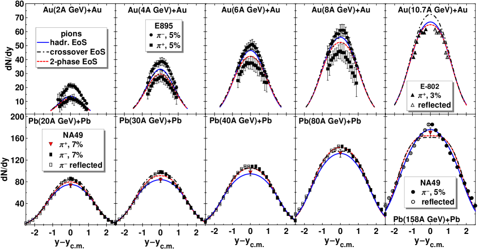
Figure 1: (Color online) Rapidity spectra of pions from central collisions of Au+Au ($b=$ 2 fm) and Pb+Pb ($b=$ 2.4 fm). Experimental data are taken for central Au+Au collisions at AGS energies Klay:2003zf (at 2$A$–8$A$ GeV, centrality 5%) and Ahle:1999jm (at 10.7$A$ GeV, centrality 3%), and Pb+Pb collisions at SPS energies Afanasiev:2002mx ; Alt:2007aa with centrality 7% at 20$A$–80$A$ GeV and centrality 5% at 158$A$ GeV.

In Fig. 1, comparison with available experimental data on rapidity distributions of pions from central collisions is presented. As particles are not isotopically distinguished in the 3FD model 3FD , only the total number of pions $N_{\pi}$ is calculated in the model. In Fig. 1, rapidity distribution of $N_{\pi}/3$ pions is displayed which, strictly speaking, should be compared with the sum of $\pi^{+}$, $\pi^{-}$ and $\pi^{0}$ distributions divided by 3. In view of the fact that the experimental $\pi^{-}$ distributions are always situated above the $\pi^{+}$ ones, a “good agreement” with the model means that calculated spectrum of $1/3$ of all pions turns out in between experimental $\pi^{+}$ and $\pi^{-}$ distributions. As seen from Fig. 1, this is always the case at AGS energies for all three EoS’s. At the SPS energies differences between predictions of different scenarios and experimental data do not exceed 10%, which is quite acceptable in view of uncertainties of the model (such as a choice of the impact parameter, accuracy of the multi-fluid approximation, phenomenological freeze-out procedure, etc.). Therefore, we can approximately conclude that the pion rapidity distributions are reasonably well reproduced by all of the considered EoS’s in the region of AGS–SPS incident energies.

A comment concerning the hadronic EoS is in order here. As it was mentioned in Refs. 3FD-2012-stopping ; 3FD , we proceeded from a principle of fair treatment of any EoS. It means that any possible uncertainties in the parameters are treated in favor of the EOS. Therefore, for the hadronic EoS the parameters of the friction enhancement and the formation time of the fireball fluid 3FD-2012-stopping ; 3FD were chosen such that the baryon stopping and the mid-rapidity pion density were reproduced at the top SPS energy of 158$A$ GeV. Thus, it is not surprising that the hadronic-EoS result is the best at 158$A$ GeV, see Fig. 1. However, even with this fit the pion distributions at midrapidity, i.e. $(\pi^{+}+\pi^{-})/2$, turn out to be somewhat underestimated at lower SPS energies, as seen in Fig. 1, and strongly overestimated at higher (RHIC) energies, as it will be seen below.

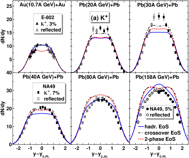
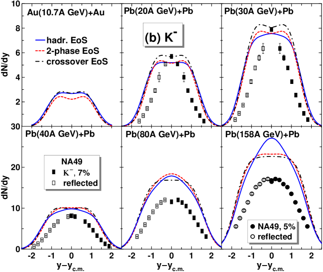
Figure 2: (Color online) Rapidity spectra of positive [(a) block of panels] and negative [(b) block panels] kaons from central collisions of Au+Au ($b=$ 2 fm) and Pb+Pb ($b=$ 2.4 fm). Experimental data are for central Au+Au collisions at AGS energy of 10.7$A$ GeV (centrality 3%) Ahle:1999jm and Pb+Pb collisions Afanasiev:2002mx ; Alt:2007aa at SPS energies with centrality 7% at 20$A$–80$A$ GeV and centrality 5% at 158$A$ GeV.

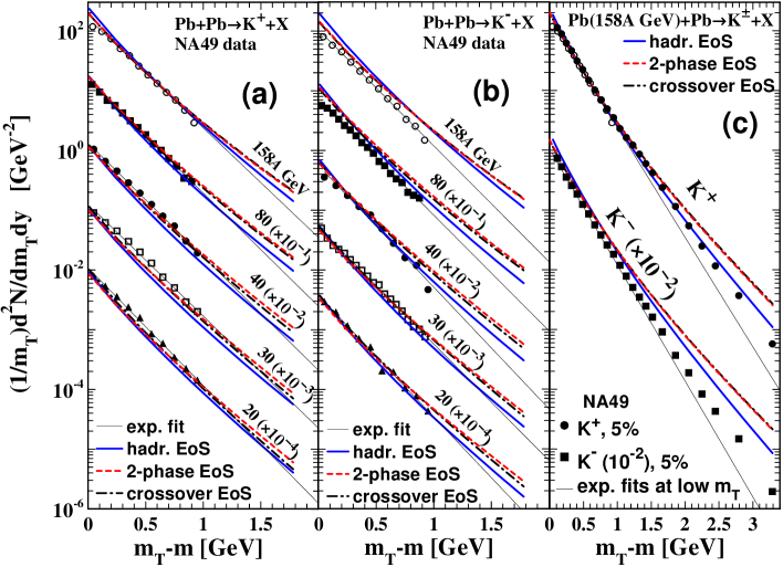
Figure 3: (Color online) Transverse mass spectra at mid-rapidity of positive (a) and negative (b) kaons from central collisions Pb+Pb ($b=$ 2.4 fm) at various incident energies and those in the extended transverse-mass range at 158$A$ GeV (c). Experimental data are taken from Refs. Afanasiev:2002mx ; Alt:2007aa and for high $p_{T}$ momenta, from Ref. Alt:2007cd .

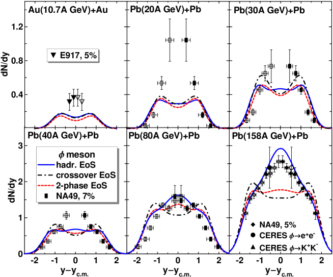
Figure 4: (Color online) Rapidity spectra of $\phi$ mesons from central collisions of Au+Au ($b=$ 2 fm) and Pb+Pb ($b=$ 2.4 fm). Experimental data for central Pb+Pb collisions at SPS energies with centrality 7% at 20$A$–80$A$ GeV and centrality 5% at 158$A$ GeV are taken Ref. Alt:2008iv and for central Au+Au collisions at 11.7$A$ GeV/c and centrality 5%, from Ref. Back:2003rw .

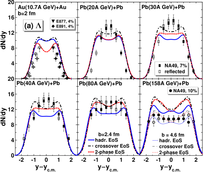
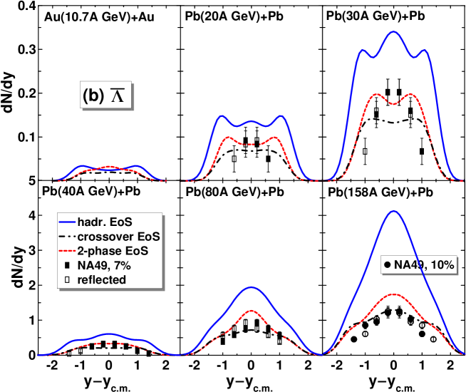
Figure 5: (Color online) Rapidity spectra of $\Lambda$ [(a) block of panels] and $\bar{\Lambda}$ [(b) block of panels] hyperons from central collisions of Au+Au ($b=$ 2 fm) and Pb+Pb ($b=$ 2.4 fm). Results for Pb+Pb collisions with $b=$ 4.6 fm are also displayed for $\Lambda$’s at 158$A$ GeV. Experimental data for central Pb+Pb collisions at SPS energies with centrality 7% at 20$A$–80$A$ GeV and centrality 10% at 158$A$ GeV are taken from Ref. Alt:2008qm , and for central Au+Au collisions at 11.5$A$ GeV/c and centrality 4%, from Ref. Barrette:2000cb .

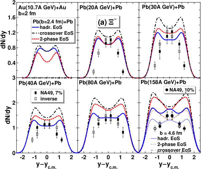
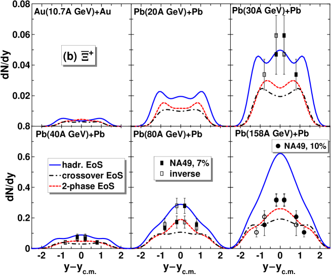
Figure 6: (Color online) Rapidity spectra of $\Xi^{-}$ [(a) block of panels] and $\bar{\Xi}^{+}$ [(b) block of panels] hyperons from central collisions of Au+Au ($b=$ 2 fm) and Pb+Pb ($b=$ 2.4 fm). Experimental data are taken for central Pb+Pb collisions Alt:2008qm at SPS energies with centrality 7% at 20$A$–80$A$ GeV and centrality 10% at 158$A$ GeV. Results for Pb+Pb collisions with $b=$ 4.6 fm are also displayed for $\Xi^{-}$’s at 158$A$ GeV.

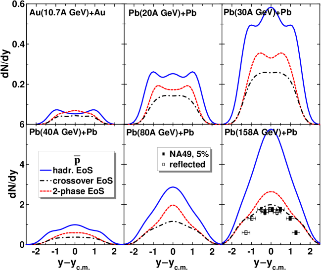
Figure 7: (Color online) Rapidity spectra of anti-protons from central collisions of Au+Au ($b=$ 2 fm) and Pb+Pb ($b=$ 2.4 fm). Experimental data for central Pb+Pb collisions at 158$A$ GeV with centrality 5% are taken from Ref. Anticic:2010mp .

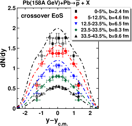
Figure 8: (Color online) Rapidity spectra of anti-protons at various centralities from collisions Pb+Pb at $E_{lab}=$ 158$A$ GeV. Experimental data are taken from Ref. Anticic:2010mp . Curves present calculations with the crossover EoS at different impact parameters ($b$).

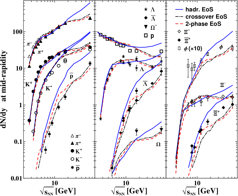
Figure 9: (Color online) Rapidity densities $dN/dy$ at mid-rapidity of various produced particles as functions of the center-of-mass energy of colliding nuclei predicted by 3FD calculations with three considered EoS’s. Experimental data are from compilation of Ref. Andronic:2005yp complemented by recent data from STAR collaboration Zhu:2012ph and latest update of the compilation of NA49 numerical results Compilation-NA49 ; Blume:2011sb .

In Fig. 2, rapidity distributions of positive and negative kaons from central collisions are presented. In fact, the model provides distributions of kaons, $K$, and antikaons, $\bar{K}$, which are sums of yields of $K^{+}+K^{0}$ and $K^{-}+\bar{K}^{0}$, respectively. The distributions of $K^{+}$ and $K^{-}$ are then approximately associated with distributions of $K$ and $\bar{K}$, respectively, divided by two. This approximation induces a certain error especially at low incident energies, where yields of $K^{+}$ and $K^{0}$ (and, correspondingly, $K^{-}$ and $\bar{K}^{0}$) noticeably differ.

As seen from Fig. 2, the $K^{-}$ production is distinctly overestimated in all of the considered scenarios. However, it is early to conclude that all the scenarios fail. This overestimation can be a consequence of the fact that the extrapolation of experimental data (the exponential one) beyond the measured points (thin solid lines in Fig. 3) essentially differs from results of calculations at high transverse masses ($m_{T}$), while in the experimentally measured low-$m_{T}$ region these are quite similar. In fact, determination of the rapidity density requires integration over $m_{T}$ up to infinity. Therefore, the experimental result can be different from the model ones because of their difference in the $m_{T}$ region, where experimental data are absent. Similar situation takes place for the $K^{+}$ yields. At lower SPS energies the experimental extrapolation to high $m_{T}$ reasonably agree with model results and hence the same reasonable agreement is observed in rapidity distributions. At higher SPS energies (80$A$ and 158$A$ GeV) the experimental (exponential) extrapolation is again distinctly lower than the model predictions. Therefore, the model rapidity distributions overestimate the experimental ones. It is worthwhile to notice that the calculated shapes of the $m_{T}$ spectra of kaons are somewhat similar to that of pion spectra, i.e. they are slightly concave in the logarithmic scale rather than linear, as it was assumed in the experimental extrapolation. Measurements of high transverse momenta later performed by NA49 collaboration at 158$A$ GeV Alt:2007cd showed that the exponential extrapolation of the low-$m_{T}$ data indeed underestimates the high-$m_{T}$ data, see (c) panel of Fig. 3. At the same time the 3FD predictions overestimate these high-$m_{T}$ data. The latter fact is expected, because even abundant hadronic species become rare species at high momenta. Therefore, their treatment on the basis of grand canonical ensemble (which is the case in the 3FD model) results in overestimation of their yield.

In view of the above possible explanation of the difference between calculated and experimental spectra it is early to conclude that the 3FD model fails to reproduce the $K^{+}$ and $K^{-}$ rapidity distributions. Again different EoS-scenarios agree (or disagree) with the available data approximately to the same extent. An important feature of the $K^{+}$ distributions is that all scenarios underestimate mid-rapidity values of the experimental data. This results in a failure to reproduce the experimental “horn” in the $K^{+}/\pi^{+}$ ratio Alt:2007aa , see sect. IV.

In Fig. 4 rapidity distributions of $\phi$ mesons from central collisions are presented. Here the situation is controversal. At high SPS energies, predictions of the hadronic EoS look certainly preferable. At lower SPS energies and the top AGS energy, predictions of different scenarios are rather similar and all of them considerably underestimate the experimental data at the mid-rapidity region. A reason of this is still unclear.

Let us turn to baryonic distributions. Since proton distributions have been already analyzed in detail in Refs. Ivanov:2012bh ; 3FD-2012-stopping , let us directly proceed to strange baryons. In Figs. 5 and 6 rapidity distributions of $\Lambda$, $\bar{\Lambda}$, $\Xi^{-}$ and $\bar{\Xi}^{+}$ hyperons from central collisions are presented. Because of the low centrality at 158$A$ GeV (10%), results for Pb+Pb collisions with $b=$ 4.6 fm are also displayed for $\Lambda$ and $\Xi^{-}$. For corresponding antiparticles $\bar{\Lambda}$ and $\bar{\Xi}^{+}$ the results with $b=$ 2.4 fm and $b=$ 4.6 fm are fairly close to each other. Therefore, calculations with $b=$ 4.6 fm are not presented. As seen, data on $\Lambda$ and $\Xi^{-}$ hyperons are reasonably reproduced by all of considered EoS’s. Apparent preference of the hadronic scenario in reproducing the $\Xi^{-}$ data cannot be considered as an argument in favor of this scenario because the extent of the overestimation by the deconfinement-transition scenarios is just within the accuracy of the grand-canonical approach. At the same time, for anti-hyperons $\bar{\Lambda}$ and $\bar{\Xi}^{+}$ the hadronic scenario evidently fails: it considerably overestimates the data, especially at the top SPS energy. The case of $\bar{\Xi}^{+}$ at 30$A$ GeV is not spectacular. There the data have too large error bars. For $\Lambda$ and $\bar{\Lambda}$ the crossover EoS looks certainly preferable. At the same time it is hardly possible to expect from the 3FD model with 2-phase and crossover EoS’s a better agreement with data on such rare probes as $\Xi^{-}$ and $\bar{\Xi}^{+}$ because the model is based on grand-canonical statistics and therefore requires “large” multiplicities to be valid.

Figure 7 confirms that the hadronic scenario strongly overestimates experimental data on antibaryons, in the present case, on antiprotons. At the same time, the crossover scenario almost perfectly reproduces the antiproton rapidity distribution even at various centralities, see Fig. 8. Correspondence between the centrality related to a data set and a mean value of the impact parameter used in the calculation is taken from Ref. Alt:2003ab .

In all the blocks of figures I kept the results for Au+Au collisions at 10$A$ GeV, even if there are no data for this reaction. This done because the deconfinement transition in the presently studied scenarios of nuclear collisions starts around this incident energy, see Refs. Ivanov:2012bh ; 3FD-2012-stopping . Therefore, it is important to observe evolution of particle distributions beginning from this energy.

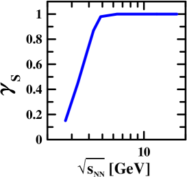
Figure 10: (Color online) Strangeness suppression factor as a function of the center-of-mass energy of colliding nuclei.

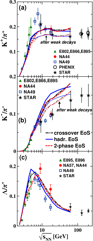
Figure 11: (Color online) The energy dependence of ratios of the rapidity densities $dN/dy$ at mid-rapidity: (a) $K^{+}$ to $\pi^{+}$, (b) $K^{-}$ to $\pi^{-}$, and (c) $\Lambda$ to $\pi^{-}$. Compilation of experimental data is from Ref. Blume:2011sb complemented by recent STAR data Zhu:2012ph ; Aggarwal:2010ig . Calculated ratios with pions including contribution from weak decays are also displayed by thin lines. The latter ratios are relevant to STAR and PHENIX data.

IV Mid-rapidity Densities and Their Ratios

Fig. 9 summarizes and extends the discussion of the previous section. It displays excitation functions of the mid-rapidity values of the rapidity spectrum of various produced particles but in a wider range of incident energies $\sqrt{s_{NN}}=$ 2.7–62.4 GeV. Results for the top calculated energy of $\sqrt{s_{NN}}=$ 62.4 GeV should be taken with care, because they are not quite accurate, as an accurate computation requires unreasonably high memory and CPU time.

The strangeness production at low incident energies is overestimated within the 3FD model. This is the consequence of the fact that the 3FD model is based on the grand canonical ensemble. This shortcoming can be easily cured by introduction of a phenomenological factor $\gamma_{S}$ Koch:1986ud which takes into account an additional strangeness suppression due to constraints of canonical ensemble. The mid-rapidity densities of single-strange particles ($K^{\pm}$, $\Lambda$ and $\bar{\Lambda}$), displayed in Fig. 9, are multiplied by $\gamma_{S}$ factor, and multi-strange particles ($\phi$, $\Xi^{-}$, $\bar{\Xi}^{+}$ and $\Omega$), by $(\gamma_{S})^{n_{s}}$ factor, where $n_{s}$ is the number of valence strange quarks contained in this particle.

The excitation function of the $\gamma_{S}$ factor is presented in Fig. 10, which is of course applicable only to central collisions of considered nuclei. On average, there is no need for additional strangeness suppression at $\sqrt{s_{NN}}>$ 5 GeV, though the reproduction of data on some strange species is still far from being perfect. The hadronic scenario looks worst in this respect. At 5 GeV $\leq\sqrt{s_{NN}}\leq$ 17 GeV, i.e. in the range of the SPS energy, it is impossible to find a unique value of $\gamma_{S}$ for this scenario to simultaneously improve reproduction of data on all of the strange hadrons. At $\sqrt{s_{NN}}\geq$ 17 GeV the hadronic scenario again requires an additional strangeness suppression. However, introduction of such a suppression at high incident energies is physically unjustified, because multiplicities of strange hadrons are already quite high for applicability of the grand canonical ensemble.

Fig. 9 confirms that the hadronic scenario considerably overestimates mid-rapidity densities of antibaryons (strange and nonstrange) predicted by EoS’s with a deconfinement transition and (as a rule) those deduced form experiment, starting already from lower SPS energies, i.e. $\approx$20$A$ GeV. At energies above the top SPS one, the mid-rapidity densities predicted by the hadronic scenario considerably exceed the data on all species. Notice that agreement of hadronic-scenario predictions with data on the major part of species in the SPS energy range was achieved at the expense of considerable enhancement the inter-fluid friction in the hadronic phase 3FD-2012-stopping ; 3FD as compared with its microscopic estimate of Ref. Sat90 . Precisely this enhancement makes bad job at energies above the SPS.

The advantage of deconfinement-transition scenarios is that they do not require any modification of the microscopic friction in the hadronic phase. They reasonably agree with all the data with the exception of negative kaons and $\phi$-mesons in the SPS energy range. A possible reason of disagreement with negative-kaon data is inaccuracy of the experimental extrapolation of the transverse-mass spectra, discussed in the previous section. As for $\phi$-mesons, the reason of this is still unclear. Rare probes, such as $\bar{\Xi}^{+}$ and $\Omega^{-}$, are also poorly reproduced, that is a consequence of inapplicability of the grand canonical ensemble for the treatment of such rare species.

In Fig. 11, ratios of various hadronic mid-rapidity densities are presented as functions of the incident energy. Calculated ratios with pions including contribution from weak decays of strange hadrons are also displayed by the corresponding thin lines. These ratios are relevant to STAR and PHENIX data Zhu:2012ph ; Aggarwal:2010ig . All of the considered scenarios do not reproduce the horn anomaly in the $K^{+}/\pi^{+}$ ratio Alt:2007aa around $E_{lab}=$ 30$A$ GeV. As it was demonstrated in Fig. 2, the reason is that all scenarios underestimate mid-rapidity values of $K^{+}$ as compared to the experimental data, while its rapidity distributions at peripheral rapidities look almost perfect. As it was found, the value of this ratio is quite insensitive to variations of the freeze-out parameter $\varepsilon_{\mbox{\scriptsize f}rz}$ 3FD-2012-stopping ; 3FD , because the yields of $K^{+}$ and $\pi^{+}$ increase or decrease proportionally with the change of $\varepsilon_{\mbox{\scriptsize f}rz}$.

Authors of Ref. Andronic:2008gu have noticed that within the statistical model the peak the $K^{+}/\pi^{+}$ ratio can be better reproduced if the contribution of the $f_{0}$(600) resonance, i.e. the $\sigma$ meson, is taken into account. However, authors of Ref. Satarov:2009zx concluded that the $\sigma$ meson does not solve the problem. In the present 3FD calculations the $\sigma$ meson is included. Moreover, the $\sigma$ spectral function is taken into account accordingly to parametrization of Ref. Wolf:1997iba .

A possible way to improve the reproduction of the horn anomaly is to accept different freeze-out conditions, i.e. energy densities $\varepsilon_{\mbox{\scriptsize f}rz}$, for $K^{+}$ and $\pi^{+}$ in this narrow energy region near $E_{lab}=$ 30$A$ GeV. However, physical reasons for such a radical solution of the horn-anomaly problem are absent. Another possibility consists in noticeable difference in $K^{+}$ and $K^{0}$ densities in this energy range. I would like to remind that the 3FD model does not distinguish isotopic states of hadrons and hence the yield of $K^{+}$ is determined as half of the total $K$ yield consisting of the sum of $K^{+}$ and $K^{0}$ contributions. Similarly, the $\pi^{+}$ yield is determined as one third of the total pion one. However, a physical reason for such an isotopic asymmetry in this narrow energy range is not seen. Moreover, such an asymmetry would be opposite to a natural isotopic asymmetry at which the $K^{0}$ yield exceeds the $K^{+}$ one. This natural asymmetry results from initial isotopic asymmetry of colliding nuclei.

A possible reason for overestimation of $K^{-}/\pi^{-}$ ratio, see (b) panel of Fig. 11, as compared with the data has been already mentioned in the previous section. It can result from difference of the extrapolation of transverse-mass experimental data (exponential extrapolation) beyond the measured points (thin solid lines in Fig. 3) from results of calculations at high transverse masses ($m_{T}$). Therefore, it would be desirable to directly compare the transverse-momentum spectra predicted by the model with experimental ones at high transverse momenta. The $\Lambda/\pi^{-}$ ratio, see (c) panel of Fig. 11, is quite satisfactorily reproduced by all of the scenarios.

V Summary

Results on rapidity distributions of particles produced in relativistic heavy-ion collisions in the energy range 2.7 GeV $\leq\sqrt{s_{NN}}\leq$ 62.4 GeV are presented. These simulations were performed within the three-fluid model 3FD employing three different equations of state: a purely hadronic EoS gasEOS and two versions of the EoS involving the deconfinement transition Toneev06 . These two versions are an EoS with the first-order phase transition and that with a smooth crossover transition. Details of these calculations are described in the first paper of this series 3FD-2012-stopping dedicated to analysis of the baryon stopping.

If was found that the model within all of the considered scenarios reproduces approximately to the same extent the available data on almost all (with some exceptions) hadronic species in the AGS–SPS energy range, i.e. at 2.7 GeV $\leq\sqrt{s_{NN}}\leq$ 17.4 GeV. In the case of the hadronic EoS this agreement is achieved at the expense of noticeable enhancement of the inter-fluid friction in the hadronic phase 3FD-2012-stopping ; 3FD as compared with its microscopic estimate of Ref. Sat90 . Reproduction of the data is better for abundant species, as it should be within grand-canonical statistics. The above mentioned exceptions are

• At lower SPS energies and the top AGS energy, predictions of all scenarios are rather similar and all of them considerably underestimate the experimental $\phi$-meson data. Moreover, at the top SPS energy, the hadronic EoS unexpectedly gives the best description of the $\phi$-meson data. The reason of this is unclear.

• The strangeness enhancement in the incident energy range near 30$A$ GeV, i.e. the “horn” anomaly in the $K^{+}/\pi^{+}$ ratio Alt:2007aa , is not reproduced in any scenario.

• The $K^{-}$ production is distinctly overestimated in all of the considered scenarios. This overestimation can be a consequence of the extrapolation of experimental data (the exponential one) beyond the measured points that essentially differs from results of calculations at high transverse masses, while in the experimentally measured low-$m_{T}$ region these are quite similar.

• Data of rare probes (like $\Xi^{-}$ and $\bar{\Xi}^{+}$ hyperons) are poorly reproduced apparently because of the grand-canonical statistics used in the 3FD model.

• The last exception concerns only the hadronic EoS. The hadronic scenario considerably overestimates experimental rapidity densities of antibaryons (both strange and nonstrange), starting already from lower SPS energies, i.e. $\approx$ 20$A$ GeV. At the same time, the deconfinement-transition scenarios successfully (to a various extent) reproduce these data.

The failure with the $\phi$-meson data and the “horn” anomaly requires further investigation. The proposed reason of the overestimation of the $K^{-}$ production also needs to be checked.

At energies above the top SPS one, i.e. at $\sqrt{s_{NN}}>$ 17.4 GeV, the mid-rapidity densities predicted by the hadronic scenario considerably exceed the available RHIC data on all the species. The deconfinement-transition scenarios reasonably agree with all the data.

The 3FD model deals with three different fluids 3FD ; 3FD-2012-stopping . These are two baryon-rich fluids initially associated with constituent nucleons of the projectile and target nuclei. These fluids are either spatially separated or unified at the freeze-out stage. In addition, newly produced particles, populating the mid-rapidity region, are associated with a baryon-free (“fireball”) fluid which remains undissolved in baryonic fluids till the freeze-out. A certain formation time $\tau$ is allowed for the fireball fluid, during which the matter of the fluid propagates without interactions. The formation time is associated with a finite time of string formation. The main difference concerning this baryon-free fluid in considered alternative scenarios consists in different formation times: $\tau=2\;\mbox{fm/c}$ for the hadronic scenario and $\tau=0.17\;\mbox{fm/c}$ for scenarios involving the deconfinement transition 3FD-2012-stopping .

As it is seen from simulations, the main contribution to baryon and meson yields comes from baryon-rich fluids within the deconfinement-transition scenarios. This contribution slowly decreases with the incident energy rise. For instance, at $\sqrt{s_{NN}}=$ 39 GeV approximately half of pions are produced from the baryon-free fluid within the deconfinement-transition scenarios. For all other particles (i.e. baryons and mesons) and lower energies this fraction is essentially lower. At the same time the fraction of half for pions from the baryon-free fluid is achieved already at $\sqrt{s_{NN}}\simeq$ 9 GeV (i.e. $E_{lab}\simeq$ 40$A$ GeV) within the hadronic scenario. This is one of the reasons why $\tau$ was chosen so large in the hadronic scenario. Large formation time prevents absorption of the baryon-free matter by the baryonic fluids. Without this large contribution of the baryon-free fluid it is impossible to reproduce mesonic yields at SPS energies within the hadronic scenario. However, this strongly developed baryon-free fluid makes bad job for antibaryons in the case of the hadronic EoS. The reason is that antibaryons are dominantly produced from the baryon-free fluid even at lower incident energies within all of the considered scenarios. Their yields in the hadronic scenario strongly overestimate experimental data. At $\sqrt{s_{NN}}>$ 17.4 GeV the overdeveloped baryon-free fluid makes already bad job for for all produced particles, resulting in considerable overestimation of the available RHIC data on all the species within the hadronic scenario.

All the above speculations are formulated in terms of the 3FD model. However, they hold true in general physical terms, if baryon-rich fluids are understood as a matter formed of leading particles, predominantly (but not solely) occupying peripheral rapidities, and the baryon-free fluid is associated with newly produced particles, predominantly (but not solely) occupying mid-rapidity region. At large baryon stopping, the difference between these groups of particles become less pronounced.

All the above results certainly indicate in favor of the deconfinement-transition scenarios, though they also are not perfect in reproduction of the data ($\phi$-meson, the “horn” anomaly). It is difficult to judge on a preference of the 2-phase or crossover EoS’s. The first-order transition in the 2-phase EoS is very abrupt. On the contrary, the crossover transition constructed in Ref. Toneev06 is very smooth Ivanov:2012bh ; 3FD-2012-stopping . In this respect, this version of the crossover EoS certainly contradicts results of the lattice QCD calculations, where a fast crossover, at least at zero chemical potential, was found Aoki:2006we . Therefore, a true EoS is somewhere in between the crossover and 2-phase EoS’s of Ref. Toneev06 .

Acknowledgements

I am grateful to A.S. Khvorostukhin, V.V. Skokov, and V.D. Toneev for providing me with the tabulated 2-phase and crossover EoS’s. The calculations were performed at the computer cluster of GSI (Darmstadt). This work was supported by The Foundation for Internet Development (Moscow) and also partially supported by the grant NS-215.2012.2.

References

- (1) Yu. B. Ivanov, Phys. Lett. B721, 123 (2013) [arXiv:1211.2579 [hep-ph]].
- (2) Yu. B. Ivanov, arXiv:1302.5766 [nucl-th], to be published in Phys. Rev. C.
- (3) Yu. B. Ivanov, V. N. Russkikh, and V.D. Toneev, Phys. Rev. C 73, 044904 (2006) [nucl-th/0503088].
- (4) V. M. Galitsky and I. N. Mishustin, Sov. J. Nucl. Phys. 29, 181 (1979).
- (5) Y. .B. Ivanov and V. N. Russkikh, PoS CPOD 07, 008 (2007) [arXiv:0710.3708 [nucl-th]].
- (6) V. N. Russkikh and Yu. B. Ivanov, Phys. Rev. C 74, 034904 (2006) [nucl-th/0606007].
- (7) Yu. B. Ivanov and V. N. Russkikh, Eur. Phys. J. A 37, 139 (2008) [nucl-th/0607070]; Phys. Rev. C 78, 064902 (2008) [arXiv:0809.1001 [nucl-th]].
- (8) Yu. B. Ivanov, I. N. Mishustin, V. N. Russkikh, and L. M. Satarov, Phys. Rev. C 80, 064904 (2009) [arXiv:0907.4140 [nucl-th]].
- (9) A. S. Khvorostukhin, V. V. Skokov, K. Redlich, and V. D. Toneev, Eur. Phys. J. C48, 531 (2006) [nucl-th/0605069].
- (10) W. Cassing and E. L. Bratkovskaya, Nucl. Phys. A831, 215 (2009) [arXiv:0907.5331 [nucl-th]].
- (11) H. Petersen, J. Steinheimer, G. Burau, M. Bleicher, and H. Stocker, Phys. Rev. C 78, 044901 (2008) [arXiv:0806.1695v3 [nucl-th]]
- (12) J. Steinheimer V. Dexheimer, H. Petersen, M. Bleicher, S. Schramm, and H. Stoecker, Phys. Rev. C 81, 044913 (2010) [arXiv:0905.3099 [hep-ph]].
- (13) E. L. Bratkovskaya, M. Bleicher, M. Reiter, S. Soff, H. Stoecker, M. van Leeuwen, S. A. Bass, and W. Cassing, Phys. Rev. C 69, 054907 (2004) [nucl-th/0402026].
- (14) H. Weber, E. L. Bratkovskaya, W. Cassing, and H. Stöcker, Phys. Rev. C 67, 014904 (2003) [nucl-th/0209079].
- (15) A. B. Larionov, O. Buss, K. Gallmeister, and U. Mosel, Phys. Rev. C 76, 044909 (2007) [arXiv:0704.1785 [nucl-th]].
- (16) M. Wagner, A. B. Larionov, and U. Mosel, Phys. Rev. C 71, 034910 (2005) [nucl-th/0411010].
- (17) Y. Hama, T. Kodama and O. Socolowski, Jr., Braz. J. Phys. 35, 24 (2005) [hep-ph/0407264].
- (18) I.N. Mishustin, V.N. Russkikh, and L.M. Satarov, Yad. Fiz. 48, 711 (1988) [Sov. J. Nucl. Phys. 48, 454 (1988)].
- (19) V. N. Russkikh, Yu. B. Ivanov, Yu. E. Pokrovsky, and P. A. Henning, Nucl. Phys. A572, 749 (1994).
- (20) I.N. Mishustin, V.N. Russkikh, and L.M. Satarov, Yad. Fiz. 54, 429 (1991) [Sov. J. Nucl. Phys. 54, 260 (1991)].
- (21) U. Katscher, D.H. Rischke, J.A. Maruhn, W. Greiner, I.N. Mishustin, and L.M. Satarov, Z. Phys. A346, 209 (1993); A. Dumitru, U. Katscher, J.A. Maruhn, H. Stöcker, W. Greiner, and D.H. Rischke, Phys. Rev. C 51, 2166 (1995) [hep-ph/9411358]; Z. Phys. A353, 187 (1995) [hep-ph/9503347].
- (22) J. Brachmann, A. Dumitru, J.A. Maruhn, H. Stöcker, W. Greiner, and D.H. Rischke, Nucl. Phys. A619, 391 (1997) [nucl-th/9703032]; M. Reiter, A. Dumitru, J. Brachmann, J.A. Maruhn, H. Stöcker, and W. Greiner, Nucl. Phys. A643, 99 (1998) [nucl-th/9806010]; M. Bleicher, M. Reiter, A. Dumitru, J. Brachmann, C. Spieles, S.A. Bass, H. Stöcker, and W. Greiner, Phys. Rev. C 59, R1844 (1999) [hep-ph/9811459]; J. Brachmann, A. Dumitru, H. Stöcker, and W. Greiner, Eur. Phys. J. A8, 549 (2000) [nucl-th/9912014].
- (23) S. Bass, et al., Prog. Part. Nucl. Phys. 41, 225 (1998).
- (24) W. Cassing and E. L. Bratkovskaya, Phys. Rept. 308, 65 (1999).
- (25) Yu. B. Ivanov, Nucl. Phys. A474, 669 (1987).
- (26) C. Nonaka and M. Asakawa, PTEP 2012, 01A208 (2012) [arXiv:1204.4795 [nucl-th]].
- (27) A. V. Merdeev, L. M. Satarov and I. N. Mishustin, Phys. Rev. C 84, 014907 (2011) [arXiv:1103.3988 [hep-ph]].
- (28) I. N. Mishustin, A. V. Merdeev and L. M. Satarov, Phys. Atom. Nucl. 75, 776 (2012) [arXiv:1012.4364 [hep-ph]].
- (29) V. N. Russkikh, Yu. B. Ivanov, Phys. Rev. C 76, 054907 (2007) [nucl-th/0611094].
- (30) Yu. B. Ivanov, V.N. Russkikh, Yad. Fiz. 72, 1288 (2009) [Phys. Atom. Nucl. 72, 1238 (2009)] [arXiv:0810.2262 [nucl-th]].
- (31) F. Cooper and G. Frye, Phys. Rev. D 10, 186 (1974).
- (32) F. Grassi, Y. Hama, and T. Kodama, Phys. Lett. B355, 9 (1995); Z. Phys. C73, 153 (1996); Yu.M. Sinyukov, S.V. Akkelin, and Y. Hama, Phys. Rev. Lett. 89, 052301 (2002) [nucl-th/0201015]; F. Grassi, Braz. J. Phys. 35, 52 (2005) [nucl-th/0412082].
- (33) H. Stocker, W. Greiner, Phys. Rept. 137, 277 (1986)
- (34) R.B. Clare and D. Strottman, Phys.Rept. 141, 177 (1986).
- (35) J. P. Bondorf, S. I. A. Garpman and J. Zimanyi, Nuclear Physics A296, 320 (1978).
- (36) P. J. Siemens and J. O. Rasmussen, Phys. Rev. Lett. 42, 880 (1979).
- (37) M. Gazdzicki and M. I. Gorenstein, Acta Phys. Polon. B 30, 2705 (1999) [arXiv:hep-ph/9803462].
- (38) C. Alt et al. [NA49 Collaboration], Phys. Rev. C 77, 024903 (2008) [arXiv:0710.0118 [nucl-ex]].
- (39) C. Alt et al. [NA49 Collaboration], Phys. Rev. C 68, 034903 (2003) [nucl-ex/0303001].
- (40) J. L. Klay et al. [E-0895 Collaboration], Phys. Rev. C 68, 054905 (2003) [nucl-ex/0306033].
- (41) L. Ahle et al. [E-802 Collaboration], Phys. Rev. C 59, 2173 (1999).
- (42) S. V. Afanasiev et al. [NA49 Collaboration], Phys. Rev. C 66, 054902 (2002) [nucl-ex/0205002].
- (43) C. Alt et al. [NA49 Collaboration], Phys. Rev. C 77, 034906 (2008) [arXiv:0711.0547 [nucl-ex]].
- (44) C. Alt et al. [NA49 Collaboration], Phys. Rev. C 78, 034918 (2008) [arXiv:0804.3770 [nucl-ex]].
- (45) C. Alt et al. [NA49 Collaboration], Phys. Rev. C 78, 044907 (2008) [arXiv:0806.1937 [nucl-ex]].
- (46) B. B. Back et al. [E917 Collaboration], Phys. Rev. C 69, 054901 (2004) [nucl-ex/0304017].
- (47) J. Barrette et al. [E877 Collaboration], Phys. Rev. C 63, 014902 (2001) [nucl-ex/0007007].
- (48) T. Anticic et al. [NA49 Collaboration], Phys. Rev. C 83, 014901 (2011) [arXiv:1009.1747 [nucl-ex]].
- (49) A. Andronic, P. Braun-Munzinger and J. Stachel, Nucl. Phys. A 772, 167 (2006) [nucl-th/0511071].
- (50) X. Zhu [STAR Collaboration], Acta Phys. Polon. Supp. 5, 213 (2012) [arXiv:1203.5183 [nucl-ex]].
- (51) C. Blume, M. Gazdzicki, B.Lungwitz, M. Mitrovski, P. Seyboth, and H. Strobele, Compilation of NA49 numerical results, https://edms.cern.ch/document/1075059
- (52) C. Blume and C. Markert, Prog. Part. Nucl. Phys. 66, 834 (2011) [arXiv:1105.2798 [nucl-ex]].
- (53) M. M. Aggarwal et al. [STAR Collaboration], Phys. Rev. C 83, 024901 (2011) [arXiv:1010.0142 [nucl-ex]].
- (54) P. Koch, B. Muller and J. Rafelski, Phys. Rept. 142, 167 (1986).
- (55) L.M. Satarov, Yad. Fiz. 52, 412 (1990) [Sov. J. Nucl. Phys. 52, 264 (1990)].
- (56) A. Andronic, P. Braun-Munzinger and J. Stachel, Phys. Lett. B 673, 142 (2009) [Erratum-ibid. B 678, 516 (2009)] [arXiv:0812.1186 [nucl-th]].
- (57) L. M. Satarov, M. N. Dmitriev and I. N. Mishustin, Phys. Atom. Nucl. 72, 1390 (2009) [arXiv:0901.1430 [hep-ph]].
- (58) G. Wolf, B. Friman and M. Soyeur, Nucl. Phys. A 640, 129 (1998) [nucl-th/9707055].
- (59) Y. Aoki, G. Endrodi, Z. Fodor, S. D. Katz and K. K. Szabo, Nature 443, 675 (2006) [hep-lat/0611014].