Single-file diffusion with non-thermal initial conditions

Abstract

Single-file diffusion is a theoretically challenging many-body problem where the calculation of even the simplest observables, e.g. mean square displacement, for a tracer particle requires a heavy mathematical machinery. There is therefore a need for simple approaches which predict qualitatively correct behaviours. Here we put forward one such method which we use to investigate the influence of non-thermal initial conditions on the dynamics of a tracer particle. With our new approach we reproduce, up to scaling, several known asymptotic results for the tracer particle mean square displacement.

I Introduction

The dynamics of diffusing particles in one dimension which are unable to pass each other, often referred to as single-file diffusion, has attracted great theoretical interest for at least 50 years, see Harris (1965); Levitt (1973); Kehr et al. (1981); Percus (1974); Hahn and Karger (1999); van Beijeren and Kutner (1985); Schütz (1997); Burlatsky et al. (1996); Alexander and Pincus (1978); Jara and Landim (2006); Arratia (1983); Kollmann (2003); Lizana and Ambjörnsson (2008); Taloni and Lomholt (2008). More recent progress in the field addresses single-file diffusion in a potential Barkai and Silbey (2009) and that of particles with different diffusion constants Lomholt et al. (2011). One of the main theoretical predictions is that a tagged (or a tracer) particle, explores the system subdiffusively even though the collective behaviour is identical to that of non-interacting particles Rödenbeck et al. (1998); Lomholt et al. (2011). The subdiffusive behaviour can be understood through the tracer particle’s velocity-velocity correlation function which is negative and decays as $t_{D}^{-3/2}$ with delay time $t_{D}$ Percus (1974); this results translates into the classical square root law for the tagged particle’s mean square discplacement ${\cal S}(t)\propto t^{1/2}$ where $t$ is time.

Nowadays single-file diffusion also finds experimental realizations. A few examples are diffusion in colloidal systems Wei et al. (2000); Lin et al. (2005), transport in microporous materials Kukla et al. (1996); Meersmann et al. (2000), and permeability of potassium ions in nerve fibres Hodgkin and Keynes (1955). Also, exclusion effects have been proposed to be of importance for transcription factor (DNA binding proteins) dynamics Li et al. (2009).

In order to calculate dynamical properties of a tagged particle in a single-file system one needs to deal with a theoretically challenging many-body problem. This typically requires rather elaborate mathematics (e.g. Harris (1965); Levitt (1973); Kollmann (2003); Lizana and Ambjörnsson (2008); Barkai and Silbey (2009)) which may cloud fundamental understanding. There is therefore a need for simplified methods that captures correct qualitative behaviour and at the same time provide new insights to the problem. A few such papers already exist Alexander and Pincus (1978); Taloni and Lomholt (2008) for thermal initial conditions and identical particles. To the best of our knowledge there has not been a similar progress on simple approaches for non-thermal initial conditions. Some aspects have, however, been addressed Barkai and Silbey (2010); Flomenbom and Taloni (2008); Lizana et al. (2010) using rather involved techniques. The main goal of this paper is to put forward a new but simple method to calculate tagged particle properties, in particular ${\cal S}(t)$, under non-thermal conditions. Our approach relies on the assumption that we can make a quasi-static approximation for the velocity-velocity autocorrelation function and set it equal to the correlation function at equilibrium. Based on this we are able to reproduce known scaling behaviours pertaining to different types of initial conditions.

II The quasi-equilibrium approach

Imagine a single-file system extending to infinity in both directions. The particles are identical, point-like and undergo Brownian motion in between hard-core repulsive interactions. Now we tag one particle, label it “0”, and place it at time $t=0$ in the origin, that is, $x_{0}(t=0)=0$. The remaining particles are initially distributed symmetrically around $x_{0}=0$, $...x_{-2},x_{-1},x_{0},x_{1},x_{2},...$, according to some non-thermal distribution $\rho_{0}(x)$. We then ask: what is the mean square displacement, ${\cal S}(t)$, of particle $0$? Here we define ${\cal S}(t)=\langle x_{0}(t)^{2}\rangle$ where $\langle...\rangle$ denotes ensemble average.

Our expression for ${\cal S}(t)$ is based on the following quasi-equilibrium argument. For an equilibrated single-file it is well known that the long time limit of the velocity-velocity correlation function for a tagged particle is Percus (1974)

$$\langle v(t)v(t-t_{D})\rangle\simeq-\sqrt{\frac{D}{\pi}}\frac{1}{4\varrho}|t_{D}|^{-3/2}$$ (1)

where $v(t)=dx(t)/dt$ and $\varrho$ is the constant average particle concentration (average inverse inter-particle distance), and $D$ is the single-particle diffusion constant (assumed equal for all particles). Now we assume that Eq. (1) holds for all, even non-thermal, initial conditions if we replace $\varrho$ with the time-dependent concentration $\rho(x,t)$ in the vicinity of the tagged particle, i.e.,

$$\varrho\rightarrow\rho(x=0,t)$$ (2)

This is a quasi-equilibrium approach which we assume to hold since concentration relaxations propagate faster than the tracer particle . Integrating Eq. (1) twice with respect to time yields ${\cal S}(t)=\int_{0}^{t}dt^{\prime}\int_{0}^{t}dt^{\prime\prime}\langle v(t^{\prime})v(t^{\prime\prime})\rangle=2\int_{0}^{t}dt^{\prime}\int_{0}^{t^{\prime}}du\langle v(t^{\prime})v(t^{\prime}-u)\rangle$. If we furthermore assume the tagged particle behaves elastically over time-scales longer than the velocity relaxation, we have $\int_{0}^{\infty}du\langle v(t)v(t-u)\rangle=0$ . This means that we can write ${\cal S}(t)=-2\int_{0}^{t}dt^{\prime}\int_{t^{\prime}}^{\infty}du\langle v(t^{\prime})v(t^{\prime}-u)\rangle$, which together with Eq. (1) and $\varrho=\rho(x=0,t^{\prime})$ gives

$${\cal S}(t)\simeq\sqrt{\frac{D}{\pi}}\int_{0}^{t}dt^{\prime}\frac{1}{\sqrt{t^{\prime}}\rho(x=0,t^{\prime})}$$ (3)

Now, since the macroscopic particle concentration in a single-file system and in a system of non-interacting particles are indistinguishable Rödenbeck et al. (1998) we can calculate $\rho(x=0,t)$ by simply solving the diffusion equation in one dimension, and subsequently setting $x=0$ in the associated solution. In effect this amounts to convoluting $\rho_{0}(x_{0})$ with a Gaussian propagator

$$\rho(x=0,t)=\int_{-\infty}^{\infty}\frac{e^{-x_{0}^{2}/(4Dt)}}{\sqrt{4\pi Dt}}\rho_{0}(x_{0})\,dx_{0},$$ (4)

Equation (3) [together with Eq. (4)] constitutes our main result. It is straightforward to see that for uniform initial densities those equations lead to classical single-file result for the mean square displacement

$${\cal S}(t)\simeq\frac{1}{\varrho}\sqrt{\frac{4Dt}{\pi}}$$ (5)

(see e.g. Harris (1965)) as it should.

III Special cases

In this section we will investigate four different types of $\rho_{0}(x_{0})$ and show that our simple model gives correct results up to scaling in $t$. Our results are summarised briefly in Tab. 1 and depicted in Fig. 1.

III.1 Exponential distribution

Here we consider the case where the initial particle density decays exponentially from the origin

$$\rho_{0}(x_{0})=\frac{N}{2\Delta}e^{-|x_{0}|/\Delta},$$ (6)

where $N$ is the number of particles and $\Delta$ is the characteristic decay length. Using this expression in Eq. (4) leads to

$$\rho(x=0,t)=\frac{N}{2\Delta}e^{t/\tau}{\rm erfc}\left(\sqrt{t/\tau}\right)$$ (7)

which together with Eq. (3) gives ${\cal S}(t)$ predicted by our model. Here we introduced

$$\tau=\frac{\Delta^{2}}{D}$$ (8)

Figure 1 (solid blue line) shows the result of a numerical integration of Eq. (3) [using Eq. (7)]. We see clearly that ${\cal S}(t)$ exhibits two regions with different dynamics with crossover time $\tau$. The limiting behaviours can be found analytically if we expand Eq. (7) in the short and long time limit: for short times ($t\ll\tau$) we get $\rho(x=0,t)\simeq N/(2\Delta)$, whereas for long times ($t\gg\tau$) $\rho(x=0,t)\simeq N/\sqrt{4\pi Dt}$. The resulting mean square displacement in the two limits reads

$${\cal S}(t)\simeq\Bigg{\{}\begin{array}[]{lll}\frac{2\Delta}{N}\sqrt{\frac{4Dt}{\pi}}&\propto\sqrt{t},&\qquad t\ll\tau\\ 2Dt/N&\propto t,&\qquad t\gg\tau\end{array}$$ (9)

This means that for short times the system is crowded enough such that we recover the known scaling with time in Eq. (5). For long times the tagged particle follows the system’s center-of-mass motion yielding ${\cal S}(t)\sim Dt/N$. For this limit we point out that C. Aslangul Aslangul (2007) obtained $\pi Dt/N$ using a more elaborate approach.

$\rho_{0}(x_{0})$	${\cal S}(t)\propto$
	$t/\tau\ll 1$	$t/\tau\gg 1$
$\frac{N}{2\Delta}e^{-|x_{0}|/\Delta}$	$\sqrt{t}$	$t$
$\frac{N}{\sqrt{2\pi\Delta^{2}}}e^{-x_{0}^{2}/(2\Delta^{2})}$	$\sqrt{t}$	$t$
$\sum_{n=-\infty}^{\infty}\delta(x_{0}-n\Delta)$	$t$	$\sqrt{t}$
$\frac{1}{\Delta}\left(\frac{|x_{0}|}{\Delta}\right)^{-\beta}$	$t^{(1+\beta)/2}$

Table 1: Summary of results ($\tau=\Delta^{2}/D$).

III.2 Gaussian distribution

In this subsection we take the particles to be initially distributed as a Gaussian around the origin

$$\rho_{0}(x_{0})=\frac{N}{\sqrt{2\pi\Delta^{2}}}e^{-x_{0}^{2}/(2\Delta^{2})}.$$ (10)

Putting this expression into Eq. (4) gives

$$\rho(x=0,t)=\frac{N}{\Delta}\sqrt{\frac{1}{2\pi(2t/\tau+1)}}$$ (11)

with $\tau$ given by Eq. (8). The resulting ${\cal S}(t)$ from Eq. (3) is shown in Fig. 1 (solid red line) where we see, again, two dynamically different regions with crossover time $\tau$. A similar analysis as in the previous subsection shows that

$${\cal S}(t)\simeq\Bigg{\{}\begin{array}[]{lll}\Delta\sqrt{8Dt}/N&\propto\sqrt{t},&\qquad t\ll\tau\\ 2Dt/N&\propto t,&\qquad t\gg\tau\end{array}$$ (12)

where we used that $\rho(x=0,t)\simeq N/(\Delta\sqrt{2\pi})$ for short times and $\rho(x=0,t)\simeq N/\sqrt{4\pi Dt}$ for long times. The crossover time as well as the limiting behaviours of ${\cal S}(t)$ are up to scaling in agreement with Barkai and Silbey (2010).

III.3 Equidistant particles

Here we address the situation where the particles are initially distributed on the line with the same distance $\Delta$ apart from each other:

$$\rho_{0}(x_{0})=\sum_{n=-\infty}^{\infty}\delta(x_{0}-n\Delta)$$ (13)

where $\delta(z)$ denotes the Dirac delta function. This case is different in one important aspect compared to the other cases in this paper: the concentration $\rho(x,t)$ in the long time limit approaches the (finite) constant $1/\Delta$ whereas in the other cases considered here $\rho(x,t)$ goes to zero. This means that we expect ${\cal S}(t)\sim\sqrt{Dt}$ for long times for the present case. If we carry out the calculation of $\rho(x=0,t)$ as before we find

$$\rho(x=0,t)=\frac{1}{\Delta}\frac{\vartheta_{3}(\sqrt{4t/\tau})}{\sqrt{4\pi t/\tau}}$$ (14)

where $\vartheta_{3}(z)$ is the elliptic Jacobi-Theta function Abramowitz and Stegun (1965)

$$\vartheta_{3}(z)=1+2\sum_{n=1}^{\infty}e^{-(n/z)^{2}}$$ (15)

The behaviour of ${\cal S}(t)$ is depicted in Fig. 1 (solid green line) where two regimes are visible once more. Using that $\rho(x=0,t)\simeq 1/\sqrt{4\pi Dt}$ for short times and $\rho(x=0,t)\simeq 1/\Delta$ in the long time limit, we obtain the short and long time asymptotics:

$${\cal S}(t)\simeq\Bigg{\{}\begin{array}[]{lll}2Dt&\propto t,&\qquad t\ll\tau\\ \Delta\sqrt{\frac{4Dt}{\pi}}&\propto\sqrt{t},&\qquad t\gg\tau\end{array}$$ (16)

The long time limit is in agreement with Lizana et al. (2010) up to scaling. However, the prefactor is a factor $\sqrt{2}$ too large compared to the correct result. Our simple model is therefore unable to account for numerical factors but gives the correct scaling behaviour in all cases we examined here.

One reason to why our method is unable to produce proper prefactors is that the density $\rho(x,t)$ does not contain all necessary information to predict the motion of the tagged particle. One way of seeing this is from the following simple example. Imagine that all particles are placed equidistantly with inter-particle distance $\Delta$. Now we draw a random number between zero and $\Delta$ from a uniform distribution and add the same random number to the position of all particles. If we average over many such subsystems we would obtain a new system with uniform density $1/\Delta$ just as in thermal equilibrium (each single-equidistant case has of course Dirac delta-peaked density). However, since each system is just the equidistant case shifted by a constant, ${\cal S}(t)$ for the averaged system will still be a factor $\sqrt{2}$ different compared to the case of thermal initial conditions. This illustrates that two cases may have the same uniform density but yet yield different prefactors to the $\sqrt{t}$ behaviour. Thus, the density $\rho(x,t)$ is by itself not sufficient to predict exact numerical prefactors. Another way of seeing that $\rho(x,t)$ does not hold all necessary information is to consider ${\cal S}(t)$ in thermal equilibrium. For this case Alexander & Pincus Alexander and Pincus (1978) argued that ${\cal S}(t)$ can be related to the density-density correlation function (dynamic structure factor) rather than the density itself. Their relation is another indication that only the density is not sufficient to predict the full ${\cal S}(t)$ but that one also need to consider density fluctuations at different locations.

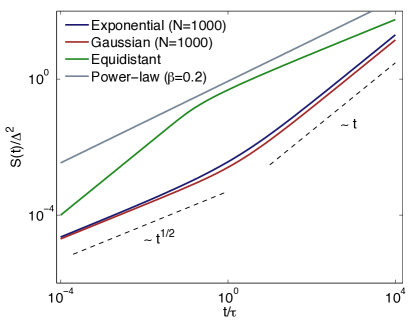
Figure 1: Mean square displacement versus time for different initial distributions $\rho_{0}(x_{0})$ ($\tau=\Delta^{2}/D$). The curves are obtained from a numerical integration of Eq. (3)

III.4 Power-law distribution

Here we investigate the scale-free initial density

$$\rho_{0}(x_{0})=\frac{1}{\Delta}\left(\frac{|x_{0}|}{\Delta}\right)^{-\beta},\ \xi<|x_{0}|<\infty,\ 0\leq\beta\leq 1$$ (17)

where we take the cut-off $\xi\to 0$. The power-law form (17) yields standard single-file dynamics [Eq. (5)] for $\beta=0$. If we put Eq. (17) into Eq. (4) we find

$$\rho(x=0,t)=\frac{1}{\sqrt{\pi}\Delta}\Gamma\left(\frac{1-\beta}{2}\right)\left(\sqrt{4t/\tau}\right)^{-\beta}$$ (18)

where $\Gamma(z)$ is the Gamma function. Using this formula in Eq. (3) leads to a mean square displacement characterized by an exponent in between that of standard and single-file diffusion. Explicitly

$${\cal S}(t)\simeq\Delta^{2}\frac{2^{1+\beta}}{(1+\beta)\Gamma\left(\frac{1-\beta}{2}\right)}(t/\tau)^{(\beta+1)/2}\propto t^{(\beta+1)/2}$$ (19)

which agrees with Barkai and Silbey (2010); Flomenbom and Taloni (2008) up to scaling.

IV Concluding remarks

In this paper we have analysed the effect of non-thermal initial conditions on the dynamics of a tagged particle in a single-file diffusion system. We used a new simple method based on a quasi-equilibrium assumption and predicted the scaling behaviour and crossover times known from literature. A future challenge will be to try to improve our method to also yield correct prefactors. The reason to why the approach works so well is that particle density relaxations decays faster than the motion of a tracer particle. It would be interesting to see how this assumption holds in other settings such a disordered single file where the diffusion constants are assigned randomly.

V Acknowledgements

We thank Ophir Flomenbom for helpful discussions. LL acknowledges the Knut and Alice Wallenberg (KAW) foundation for financial support. TA is grateful to KAW and the Swedish Research Council for funding.

References

- Harris (1965) T. Harris, Journal of Applied Probability 2, 323 (1965).
- Levitt (1973) D. Levitt, Physical Review A 8, 3050 (1973).
- Kehr et al. (1981) K. Kehr, R. Kutner, and K. Binder, Physical Review B 23, 4931 (1981).
- Percus (1974) J. Percus, Physical Review A 9, 557 (1974).
- Hahn and Karger (1999) K. Hahn and J. Karger, Journal of Physics A: Mathematical and General 28, 3061 (1999).
- van Beijeren and Kutner (1985) H. van Beijeren and R. Kutner, Physical review letters 55, 238 (1985).
- Schütz (1997) G. Schütz, Journal of statistical physics 88, 427 (1997).
- Burlatsky et al. (1996) S. Burlatsky, G. Oshanin, M. Moreau, and W. Reinhardt, Physical Review E 54, 3165 (1996).
- Alexander and Pincus (1978) S. Alexander and P. Pincus, Physical Review B 18, 2011 (1978).
- Jara and Landim (2006) M. Jara and C. Landim, in Annales de l’Institut Henri Poincare (B) Probability and Statistics (Elsevier, 2006), vol. 42, pp. 567–577.
- Arratia (1983) R. Arratia, The Annals of Probability pp. 362–373 (1983).
- Kollmann (2003) M. Kollmann, Physical review letters 90, 180602 (2003).
- Lizana and Ambjörnsson (2008) L. Lizana and T. Ambjörnsson, Physical review letters 100, 200601 (2008).
- Taloni and Lomholt (2008) A. Taloni and M. A. Lomholt, Physical Review E 78, 051116 (2008).
- Barkai and Silbey (2009) E. Barkai and R. Silbey, Physical review letters 102, 50602 (2009).
- Lomholt et al. (2011) M. Lomholt, L. Lizana, and T. Ambjörnsson, The Journal of chemical physics 134, 045101 (2011).
- Rödenbeck et al. (1998) C. Rödenbeck, J. Kärger, and K. Hahn, Physical Review E 57, 4382 (1998).
- Wei et al. (2000) Q. Wei, C. Bechinger, and P. Leiderer, Science 287, 625 (2000).
- Lin et al. (2005) B. Lin, M. Meron, B. Cui, S. Rice, and H. Diamant, Physical review letters 94, 216001 (2005).
- Kukla et al. (1996) V. Kukla, J. Kornatowski, D. Demuth, I. Girnus, H. Pfeifer, L. Rees, S. Schunk, K. Unger, J. Karger, et al., Science (New York, NY) 272, 702 (1996).
- Meersmann et al. (2000) T. Meersmann, J. Logan, R. Simonutti, S. Caldarelli, A. Comotti, P. Sozzani, L. Kaiser, and A. Pines, The Journal of Physical Chemistry A 104, 11665 (2000).
- Hodgkin and Keynes (1955) A. Hodgkin and R. Keynes, The Journal of physiology 128, 61 (1955).
- Li et al. (2009) G. Li, O. Berg, and J. Elf, Nature Physics 5, 294 (2009).
- Barkai and Silbey (2010) E. Barkai and R. Silbey, Physical Review E 81, 041129 (2010).
- Flomenbom and Taloni (2008) O. Flomenbom and A. Taloni, EPL (Europhysics Letters) 83, 20004 (2008).
- Lizana et al. (2010) L. Lizana, T. Ambjörnsson, A. Taloni, E. Barkai, and M. Lomholt, Physical Review E 81, 051118 (2010).
- Aslangul (2007) C. Aslangul, EPL (Europhysics Letters) 44, 284 (2007).
- Abramowitz and Stegun (1965) M. Abramowitz and I. Stegun, Handbook of mathematical functions: with formulas, graphs, and mathematical tables, vol. 55 (Dover publications, 1965).