The speed of interfacial waves
polarized in a symmetry plane

Abstract

The surface-impedance matrix method is used to study interfacial waves polarized in a plane of symmetry of anisotropic elastic materials. Although the corresponding Stroh polynomial is a quartic, it turns out to be analytically solvable in quite a simple manner. A specific application of the result concerns the calculation of the speed of a Stoneley wave, polarized in the common symmetry plane of two rigidly bonded anisotropic solids. The corresponding algorithm is robust, easy to implement, and gives directly the speed (when the wave exists) for any orientation of the interface plane, normal to the common symmetry plane. Through the examples of the couples (Aluminum)-(Tungsten) and (Carbon/epoxy)-(Douglas pine), some general features of a Stoneley wave speed are verified: the wave does not always exist; it is faster than the slowest Rayleigh wave associated with the separated half-spaces.

Keywords: Interfacial waves; Bi-material; Surface-impedance matrix; Stroh formalism; Anisotropic elasticity.

1 Introduction

The semiconductor industry makes great use of wafer bonding, a process which allows two different materials to be rigidly and permanently bonded along a plane interface, thus producing a composite bi-material [1]. Worldwide, there are now several hundreds of wafer bonding patents deposited yearly [2]. A similar process, fusion bonding, is used by the polymer industry to bring together two parts of different solid polymers, thus enabling the manufacture of a heterogeneous bi-material with specific properties [3, 4]. In the first case, wafers of two different crystals are stuck together through van der Waals forces, after their surface has been mirror-polished; in the second context, a fusion process takes place at the interface, followed by a cooling and consolidating period. Whichever the process, it seems important to be able to inspect the strength of the bonding, possibly through non-destructive ultrasonic evaluation. This is where the study of Stoneley waves (rigid contact) and of slip waves (sliding contact) is relevant (see Rokhlin et al. [5, 6] or Lee and Corbly [7]). In the continuum mechanics literature, great contributions can be found on the theoretical apprehension of these waves. In particular, Barnett et al. [8] for Stoneley waves and Barnett et al. [9] for slip waves have provided a rigorous and elegant corpus of results for their possible existence and uniqueness, based on the Stroh formalism [10, 11]. However very few simple numerical “recipes” exist to compute the speed (and then the attenuation factors, partial modes, and profiles) of these waves when they exist.

When the two materials have at least orthorhombic symmetry and their crystallographic axes are aligned, the analysis can be conducted in explicit form as is best summarized in the article by Chevalier et al. [12]. This explicit analysis is possible because for waves proportional to $\exp ik(x_{1}+px_{2}-vt)$ where $k$, $p$, $v$ are the respective wave number, attenuation factor, and speed of the wave, and $x_{1}$, $x_{2}$ (aligned with two common crystallographic axes) are the respective directions of propagation and attenuation, the equations of motion lead to a propagation condition which is a quadratic in $p^{2}$; then the relevant roots $p$ can be found in terms of the stiffnesses $C_{ij}$, $C^{*}_{ij}$ for each half-space, of the mass densities $\rho$, $\rho^{*}$, and of the speed $v$. After construction of the general solution to the equations of motion (a linear superposition of the partial modes), the boundary condition at the interface (rigid or sliding contact) yields the secular equation, of which $v$ is a root. If the crystallographic axes of the two orthorhombic materials do not coincide, or when at least one material is monoclinic or triclinic, then the situation becomes much more intricate. In the very particular case where the bi-material is made of the same material above and below the plane interface, with crystallographic axes symmetrically misoriented, a Stoneley wave can be found along the bisectrix of the misorientation angle [13, 14, 15]. Otherwise, analytical methods fail because in general the propagation condition is a sextic in $p$, unsolvable [16] in the Galois sense.

Now consider the case of a bi-material made of two different anisotropic half-spaces with a common symmetry plane $Z=0$, orthogonal to the interface, and with only one common crystallographic axis (the $Z$ axis), see Figure 1.

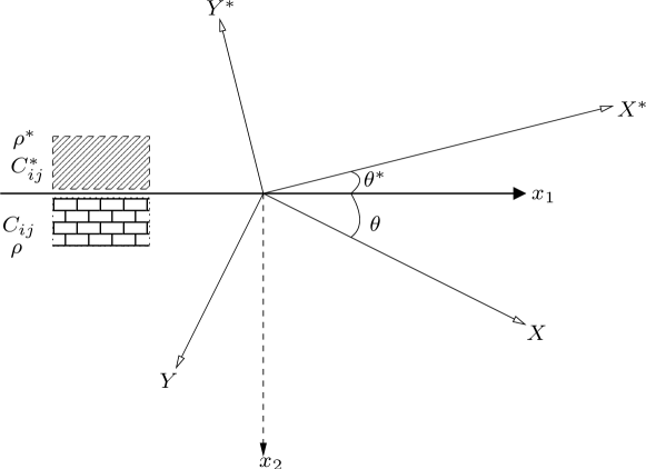
Fig. 1: Plane interface (at $x_{2}=0$) between two different anisotropic materials with a common symmetry plane (at $Z=0$).

Then the in-plane strain decouples from the anti-plane strain [10] and in each half-space, the propagation condition factorizes into the product of a quadratic in $p$ (associated with the anti-plane strain) and a quartic in $p$ (associated with the in-plane strain). Solving analytically this quartic and identifying the two qualifying roots unambiguously in order to be able to write down the boundary condition may have seemed a formidable task. However, it was recently shown in Fu [17] that such a quartic can in fact be solved and the two qualifying roots identified in quite a simple manner, using results from algebra. Once the roots $p$ are known, the complete resolution of the problem flows out naturally because the surface-impedance matrices $M(v)$ and $M^{*}(v)$ for each region are now known explicitly. This knowledge gives in turn an explicit secular equation, in the form $f(v)=0$ for some function $f$. For Stoneley waves, $f$ is a monotone decreasing function of $v$, whose only zero, when it exists, is the wave speed. This latter property is worth emphasizing: therein lies the superiority of the explicit surface-impedance matrix method above others based on algebraic manipulations which ultimately lead to a multitude of secular equations [18, 19] and/or of spurious roots [20, 21, 22, 23, 14, 24, 25, 26].

This contribution builds on recent advances by Fu and Mielke [27], Mielke and Fu [28], and Fu [17], themselves resting on the major works by Barnett and Lothe [29], Chadwick and Smith [30], Ting [11], and Mielke and Sprenger [31]. We aim at keeping the algebra to a minimum and at delivering a numerical recipe giving the wave speed in a robust manner. The reader who is keen on implementing such procedures may skip the next two sections to jump directly to Section 4, where they are summarized and presented for the Rayleigh wave speed and for the Stoneley wave speed. Section 2 recapitulates the basic equations of motion and presents the surface-impedance matrices. In Section 3, the quartic evoked above is derived, and then explicitly solved for the roots which allow for a localization of the wave near the interface. Finally, using the “recipes” of Section 4, examples of Rayleigh and Stoneley wave speeds computations are presented in Section 5, and the connection is made with some numerical results of Chevalier et al. [12].

2 Governing equations

Consider a bi-material made of two distinct anisotropic materials with a common symmetry plane, bonded rigidly along a plane interface, $x_{2}=0$ say. Let $\rho$ and $C_{ijks}$ be the mass density and elastic stiffnesses of the body below ($x_{2}\geq 0$) and $\rho^{*}$ and $C^{*}_{ijks}$ be those of the body above ($x_{2}\leq 0$). The $C_{ijks}$ and $C^{*}_{ijks}$ are assumed to satisfy the symmetry relations

$$C_{ijks}=C_{ksij}=C_{jiks},\quad\text{and}\quad C^{*}_{ijks}=C^{*}_{ksij}=C^{*}_{jiks},$$ (1)

and the strong convexity conditions

$$C_{ijks}\xi_{ij}\xi_{ks}>0,\quad C^{*}_{ijks}\xi_{ij}\xi_{ks}>0,\quad\forall\hbox{ non-zero real symmetric tensors }\mbox{\boldmath{$\xi$}}.$$ (2)

The strong ellipticity conditions are given by

$$C_{ijks}\eta_{i}\eta_{k}\gamma_{j}\gamma_{s}>0,\quad C^{*}_{ijks}\eta_{i}\eta_{k}\gamma_{j}\gamma_{s}>0,\quad\forall\hbox{ non-zero real vectors }\mbox{\boldmath{$\eta$}}\text{ and }\mbox{\boldmath{$\gamma$}},$$ (3)

and are implied by the strong convexity conditions (2). Let $XYZ$ and $X^{*}Y^{*}Z$ be along the crystallographic axes of each material; the $X$ axis ($X^{*}$ axis) makes an angle $\theta$ ($\theta^{*}$) with the interface, and $Z$ is normal to their common symmetry plane and to $x_{2}$. Finally, let $x_{1}$ be an axis such that $x_{1}x_{2}Z$ is a rectangular coordinate system. See Figure 1.

In this context, an interfacial wave is a two-component [10] inhomogeneous plane wave, whose propagation is governed by the equations of motion for the mechanical displacement ${\mbox{\boldmath{$u$}}}(x_{1},x_{2},t)=[u_{1},u_{2}]^{T}$,

$$C_{ijks}u_{k,sj}=\rho\ddot{u}_{i}\quad(x_{2}\geq 0),\quad C^{*}_{ijks}u_{k,sj}=\rho^{*}\ddot{u}_{i}\quad(x_{2}\leq 0),$$ (4)

and which decays away from the interface,

$${\mbox{\boldmath{$u$}}}\rightarrow\mathbf{0}\quad\text{as}\quad x_{2}\rightarrow\pm\infty.$$ (5)

Here and henceforward, a comma denotes differentiation with respect to spatial coordinates and a dot denotes material time derivative. Since the surfaces of the upper half-space and of the lower half-space have unit normals ($\delta_{2i}$) and $(-\delta_{2i})$, respectively, the traction vectors on these two surfaces are

$$t_{i}=-C_{i2ks}u_{k,s},\quad t^{*}_{i}=C^{*}_{i2ks}u_{k,s},\quad i=1,2,$$ (6)

and by (5), they also decay,

$$t_{i}\rightarrow 0\quad\text{as}\quad x_{2}\rightarrow+\infty,\quad t^{*}_{i}\rightarrow 0\quad\text{as}\quad x_{2}\rightarrow-\infty.$$ (7)

Without loss of generality, the interfacial wave is assumed to propagate along the $x_{1}$-direction and to have unit wave number, so that

$${\mbox{\boldmath{$u$}}}={\mbox{\boldmath{$z$}}}({\it i}x_{2}){\rm e}^{{\it i}(x_{1}-vt)}+{\rm c.c.},$$ (8)

where $v$ is the propagation speed and “c.c.” denotes the complex conjugate of the preceding term.

Substituting (8) into (4) and (6)₁ gives

$${T}{\mbox{\boldmath{$z$}}}^{\prime\prime}+({R}+{R}^{T}){\mbox{\boldmath{$z$}}}^{\prime}+({Q}-\rho v^{2}{I}){\mbox{\boldmath{$z$}}}={\bf 0},\quad x_{2}\geq 0,$$ (9)

and

$${\mbox{\boldmath{$t$}}}=-{\it i}{\mbox{\boldmath{$l$}}}({\it i}x_{2}){\rm e}^{{\it i}(x_{1}-vt)}+{\rm c.c.},$$ (10)

where

$${\mbox{\boldmath{$l$}}}={T}{\mbox{\boldmath{$z$}}}^{\prime}+{R}^{T}{\mbox{\boldmath{$z$}}},$$ (11)

a prime signifies differentiation with respect to the argument ${\it i}x_{2}$, and the $2\times 2$ matrices ${T},{R},{Q}$ are defined by their components,

$$T_{ik}=C_{i2k2},\quad R_{ik}=C_{i1k2},\quad Q_{ik}=C_{i1k1}.$$ (12)

Identical results apply for the upper half-space $x_{2}\leq 0$, with each quantity replaced by its starred counterpart, except that ${\mbox{\boldmath{$t$}}}^{*}$ is given by

$${\mbox{\boldmath{$t$}}}^{*}={\it i}{\mbox{\boldmath{$l$}}}^{*}({\it i}x_{2}){\rm e}^{{\it i}(x_{1}-vt)}+{\rm c.c.}$$ (13)

Note that satisfaction of the strong ellipticity conditions (3) ensures that $T$, $T^{*}$, and $Q$, $Q^{*}$ are all positive definite and hence invertible.

The surface-impedance matrices $M(v)$ and $M^{*}(v)$ are defined by

$$-{\it i}{\mbox{\boldmath{$l$}}}(0)=M(v){\mbox{\boldmath{$z$}}}(0),\quad{\it i}{\mbox{\boldmath{$l$}}}^{*}(0)=M^{*}(v){\mbox{\boldmath{$z$}}}^{*}(0).$$ (14)

In the Stroh [10] formulation, the second-order differential equation (9) is written as a system of first-order differential equations for the variables $z$ and $l$. Thus, for the lower half-space (and similarly for the upper half-space),

$${\mbox{\boldmath{$\xi$}}}^{\prime}=N{\mbox{\boldmath{$\xi$}}},\quad\text{where}\quad{\mbox{\boldmath{$\xi$}}}=\begin{bmatrix}{\mbox{\boldmath{$z$}}}\\ {\mbox{\boldmath{$l$}}}\end{bmatrix},\quad N=\begin{bmatrix}N_{1}&N_{2}\\ N_{3}+\rho v^{2}I&N_{1}^{T}\end{bmatrix},$$ (15)

and

$$N_{1}=-T^{-1}R^{T},\quad N_{2}=T^{-1},\quad N_{3}=RT^{-1}R^{T}-Q.$$ (16)

Here $I$ is the $2\times 2$ identity matrix.

An important property of the surface impedance matrix is that it is independent of the depth, that is

$$-{\mbox{\boldmath{$l$}}}(ix_{2})=M{\mbox{\boldmath{$z$}}}(ix_{2}),$$ (17)

see Ingebrigsten and Tonning [32]. On substituting (17) into (15) and eliminating ${\mbox{\boldmath{$z$}}}^{\prime}$, we obtain

$$\left\{(M-iR)T^{-1}(M+iR^{T})-Q+\rho v^{2}\right\}{\mbox{\boldmath{$z$}}}(ix_{2})=\mathbf{0}.$$ (18)

Since ${\mbox{\boldmath{$z$}}}(ix_{2})$ is arbitrary, it then follows that

$$(M-iR)T^{-1}(M+iR^{T})-Q-\rho v^{2}I=0.$$ (19)

This simple matrix equation satisfied by $M$ was seemingly first derived by Biryukov [33], and later rediscovered by Fu and Mielke [27] where it was shown how this equation could be exploited to compute the surface speed.

The general solution of (15) can be constructed by first looking for a partial mode solution of the form

$${\mbox{\boldmath{$\xi$}}}({\it i}x_{2})={\rm e}^{{\it i}px_{2}}{\mbox{\boldmath{$\zeta$}}},$$ (20)

say, where $p$ is a constant scalar (attenuation factor) and $\zeta$ is a constant vector to be determined. Substituting (20) into (15) leads to the eigenvalue problem $(N-pI_{4\times 4}){\mbox{\boldmath{$\zeta$}}}={\mbox{\boldmath{$0$}}}$. Under the assumption of strong ellipticity, the eigenvalues of $N$ appear as two pairs of complex conjugates when $v=0$ and they remain so until $v=v_{c}$, where $v_{c}$ is referred to as the limiting speed. In this paper we are only concerned with the subsonic case, for which $0\leq v<v_{c}$. The solution (20) decays as $x_{2}\rightarrow\infty$ only if the imaginary part of $p$ is positive. Thus, denoting by $p_{1}$, $p_{2}$ the two eigenvalues of $N$ with positive imaginary parts, and by ${\mbox{\boldmath{$\zeta$}}}^{(1)}$, ${\mbox{\boldmath{$\zeta$}}}^{(2)}$ the corresponding eigenvectors, a general decaying solution is given by

$${\mbox{\boldmath{$\xi$}}}({\it i}x_{2})=c_{1}{\rm e}^{{\it i}p_{1}x_{2}}{\mbox{\boldmath{$\zeta$}}}^{(1)}+c_{2}{\rm e}^{{\it i}p_{2}x_{2}}{\mbox{\boldmath{$\zeta$}}}^{(2)},$$ (21)

where $c_{1}$, $c_{2}$ are disposable constants. Hence at the interface,

$${\mbox{\boldmath{$\xi$}}}(0)=c_{1}{\mbox{\boldmath{$\zeta$}}}^{(1)}+c_{2}{\mbox{\boldmath{$\zeta$}}}^{(2)}=\begin{bmatrix}A\\ B\end{bmatrix}{\mbox{\boldmath{$c$}}},$$ (22)

where the $2\times 2$ matrices $A$, $B$ and the column vector $c$ are defined by

$$\begin{bmatrix}A\\ B\end{bmatrix}=\left[{\mbox{\boldmath{$\zeta$}}}^{(1)}|{\mbox{\boldmath{$\zeta$}}}^{(2)}\right],\quad{\mbox{\boldmath{$c$}}}=\begin{bmatrix}c_{1}\\ c_{2}\end{bmatrix}.$$ (23)

It follows from (22) that

$$-{\it i}{\mbox{\boldmath{$l$}}}(0)=-{\it i}B{\mbox{\boldmath{$c$}}}=-{\it i}BA^{-1}{\mbox{\boldmath{$z$}}}(0),$$ (24)

and so from (14) that

$$M(v)=-{\it i}BA^{-1},$$ (25)

which is a well-known representation of the surface-impedance matrix. As is recalled later in the paper, the surface-impedance matrices are crucial to the determination of the interfacial wave speed. In fact, if their explicit expressions are found, then an exact secular equation (an equation of which the wave speed is the only zero) is also found explicitly.

3 Explicit expressions for the surface-impedance matrices

Here it is seen that the relevant roots to the characteristic equation $\text{det}(N-pI_{4\times 4})=0$ can be obtained explicitly, without the uncertainty which one encounters in, for instance, solving a cubic for $p^{2}$. Indeed, because the characteristic equation is a quartic in $p$, the qualifying roots are those with a positive (negative) imaginary part to ensure decay with distance from the interface in the lower (upper) half-space. Thus, for the lower half-space say, they must be of the form $\alpha_{1}+i\beta_{1}$, $\alpha_{2}+i\beta_{2}$, where $\beta_{1}$ and $\beta_{2}$ are positive real numbers. This situation is in sharp contrast with the case of a wave propagating in a symmetry plane; then the characteristic equation is a cubic in $p^{2}$ and the relevant roots for the lower half-space can come in one of two forms: either as ${\it i}\alpha_{1}$, ${\it i}\alpha_{2}$, ${\it i}\alpha_{3}$, where $\alpha_{1}$, $\alpha_{2}$, $\alpha_{3}$ are positive, or as ${\it i}\alpha_{1}$, $\pm\alpha+i\beta$, where $\alpha_{1}$ and $\beta$ are positive. Although the roots of a cubic are seemingly easier to obtain analytically than those of a quartic, determining which of these two forms applies is a tricky matter. Here, once $p_{1}$, $p_{2}$ and $p_{1}^{*}$, $p_{2}^{*}$ are known, $M(v)$ and $M^{*}(v)$ can be constructed and the interfacial wave speed can be computed directly. The analysis below is conducted for the lower half-space ($x_{2}\geq 0$) and indications are given at the end of the section on how to adapt it to the upper half-space.

First write the four-component vectors ${\mbox{\boldmath{$\zeta$}}}^{(1)}$ and ${\mbox{\boldmath{$\zeta$}}}^{(2)}$ as

$${\mbox{\boldmath{$\zeta$}}}^{(1)}=\begin{bmatrix}{\mbox{\boldmath{$a$}}}^{(1)}\\ {\mbox{\boldmath{$b$}}}^{(1)}\end{bmatrix},\quad{\mbox{\boldmath{$\zeta$}}}^{(2)}=\begin{bmatrix}{\mbox{\boldmath{$a$}}}^{(2)}\\ {\mbox{\boldmath{$b$}}}^{(2)}\end{bmatrix}.$$ (26)

The vectors ${\mbox{\boldmath{$a$}}}^{(1)}$, ${\mbox{\boldmath{$a$}}}^{(2)}$ are determined from (9), that is from

$$[p_{k}^{2}{T}+p_{k}({R}+{R}^{T})+{Q}-\rho v^{2}I]{\mbox{\boldmath{$a$}}}^{(k)}={\bf 0},\quad k=1,2,$$ (27)

and the vectors ${\mbox{\boldmath{$b$}}}^{(1)}$, ${\mbox{\boldmath{$b$}}}^{(2)}$, are computed from (11) according to

$${\mbox{\boldmath{$b$}}}^{(k)}=(p_{k}{T}+{R}^{T}){\mbox{\boldmath{$a$}}}^{(k)},\quad k=1,2.$$ (28)

It then follows from (23) that

$$A=\left[{\mbox{\boldmath{$a$}}}^{(1)}|{\mbox{\boldmath{$a$}}}^{(2)}\right],\quad B=\left[{\mbox{\boldmath{$b$}}}^{(1)}|{\mbox{\boldmath{$b$}}}^{(2)}\right]=TA\Omega+R^{T}A,$$ (29)

where

$$\Omega=\begin{bmatrix}p_{1}&0\\ 0&p_{2}\end{bmatrix}.$$ (30)

The two eigenvalues $p_{1}$ and $p_{2}$ are determined from $\text{det }(N-pI)=0$, or equivalently, from

$$\text{det }[p^{2}{T}+p({R}+{R}^{T})+{Q}-\rho v^{2}I]=0.$$ (31)

This characteristic equation, called the propagation condition, is a quartic which can be written as

$$p^{4}+d_{3}p^{3}+d_{2}p^{2}+d_{1}p+d_{0}=0,$$ (32)

say, where $d_{0},d_{1},d_{2},d_{3}$ are real constants.

The usual strategy for solving a quartic equation such as (32) is to use a substitution to eliminate the cubic term; see Bronshtein and Semendyayev [34]. Thus, with the substitution $p=q-d_{3}/4$, equation (32) reduces to

$$q^{4}+rq^{2}+sq+h=0,$$ (33)

where

$$r=d_{2}-\textstyle{\frac{3}{8}}d_{3}^{2},\quad s=d_{1}-\textstyle{\frac{1}{2}}d_{2}d_{3}+\textstyle{\frac{1}{8}}d_{3}^{2},\quad h=d_{0}-\textstyle{\frac{1}{4}}d_{1}d_{3}+\textstyle{\frac{1}{16}}d_{2}d_{3}^{2}-\textstyle{\frac{3}{256}}d_{3}^{4}.$$ (34)

The behavior of the roots of (33) depends on the cubic resolvent

$$z^{3}+2rz^{2}+(r^{2}-4h)z-s^{2}=0.$$ (35)

In particular, Eq.(33), and hence Eq.(32), have two pairs of complex conjugate solutions if and only if (35) has three real roots $z_{1}$, $z_{2}$, $z_{3}$ such that $z_{2}<z_{3}\leq 0\leq z_{1}$. Then,

$$p_{1}=\textstyle{\frac{1}{2}}[\text{sign}(s)\sqrt{z_{1}}+{\it i}(\sqrt{-z_{2}}+\sqrt{-z_{3}})]-\dfrac{d_{3}}{4},$$

$$p_{2}=\textstyle{\frac{1}{2}}[-\text{sign}(s)\sqrt{z_{1}}+{\it i}(\sqrt{-z_{2}}-\sqrt{-z_{3}})]-\dfrac{d_{3}}{4},$$ (36)

where $\text{sign}(s)$ equals 1 if $s$ is non-negative and $-1$ otherwise (this definition overrides the standard definition in which $\text{sign}(0)=0$). The three roots of (35) are

$$2\lambda^{1/3}\cos(\phi)-\textstyle{\frac{2}{3}}r,\quad 2\lambda^{1/3}\cos(\phi+2\pi/3)-\textstyle{\frac{2}{3}}r,\quad 2\lambda^{1/3}\cos(\phi+4\pi/3)-\textstyle{\frac{2}{3}}r,$$ (37)

where

$$\lambda=\textstyle{\frac{1}{27}}(12h+r^{2})^{3/2},\quad\cos 3\phi=\textstyle{\frac{27}{2}}(12h+r^{2})^{-3/2}(\textstyle{\frac{2}{27}}r^{3}+s^{2}-\textstyle{\frac{8}{3}}rh).$$ (38)

Without loss of generality it can be assumed that $0\leq 3\phi\leq\pi$. It is easy to show that in this interval,

$$\cos(\phi+2\pi/3)\leq\cos(\phi+4\pi/3)\leq\cos\phi.$$ (39)

It then follows that the three roots of (35) can explicitly be identified as

$$z_{1}=2\lambda^{1/3}\cos(\phi)-\textstyle{\frac{2}{3}}r,$$

$$z_{2}=2\lambda^{1/3}\cos(\phi+2\pi/3)-\textstyle{\frac{2}{3}}r,$$

$$z_{3}=2\lambda^{1/3}\cos(\phi+4\pi/3)-\textstyle{\frac{2}{3}}r.$$ (40)

Since $z_{2}\neq z_{3}$, we may further deduce that $\phi\neq 0$ so that $0<\phi\leq\pi/3$.

Now all the ingredients are in place to compute explicitly $p_{1}$, $p_{2}$; then $A$, $B$; and ultimately, $M(v)$, which is all that is required to find the speed of the Rayleigh wave propagating at the interface between the lower half-space and a vacuum. To compute the speed of Stoneley waves and slip waves, $M^{*}(v)$ is needed. For the upper half-space $x_{2}\leq 0$, the analysis above can be repeated by starring all the quantities involved. Now the qualifying roots $p_{1}^{*}$, $p_{2}^{*}$ must have negative imaginary parts in order to satisfy the decaying condition and so (36) is replaced by

$$p^{*}_{1}=\textstyle{\frac{1}{2}}[\text{sign}(s^{*})\sqrt{z^{*}_{1}}-{\it i}(\sqrt{-z^{*}_{2}}+\sqrt{-z^{*}_{3}})]-\dfrac{d^{*}_{3}}{4},$$

$$p^{*}_{2}=\textstyle{\frac{1}{2}}[-\text{sign}(s^{*})\sqrt{z^{*}_{1}}-{\it i}(\sqrt{-z^{*}_{2}}-\sqrt{-z^{*}_{3}})]-\dfrac{d^{*}_{3}}{4}.$$ (41)

As a result, $M^{*}(v)$ can be obtained from $M(v)$ by first replacing the material constants by their starred counterparts and then taking the complex conjugate.

4 How to find the wave speed

This section presents simple algorithms that can be used to compute directly the surface wave speed and the interfacial wave speed. They rely on the use of a symbolic manipulation package such as Mathematica. The algorithm for Rayleigh waves (solid/vacuum interface) is presented in detail, and then modified for Stoneley waves (rigid solid/solid interface).

4.1 Rayleigh waves

A Rayleigh wave satisfies the traction free boundary condition ${\mbox{\boldmath{$l$}}}(\mathbf{0})={\bf 0}$. Thus, from (14)₁, its speed is given by

$$\text{det }M(v)=\text{det }(-{\it i}BA^{-1})=-\text{det }(TA\Omega A^{-1}+R^{T})=0.$$ (42)

Given a set of material constants $C_{ijkl}$ and $\rho$, the unique surface-wave speed is found by using the following robust numerical procedure:

1. Enter the values of the stiffnesses into the definitions (12) of $T$, $R$, $Q$, that is

   $$Q=\begin{bmatrix}C_{1111}&C_{1112}\\ C_{1112}&C_{1212}\end{bmatrix},\quad R=\begin{bmatrix}C_{1112}&C_{1122}\\ C_{1212}&C_{2212}\end{bmatrix},\quad T=\begin{bmatrix}C_{1212}&C_{1222}\\ C_{1222}&C_{2222}\end{bmatrix}.$$

2. Expand the quartic (31) in $p$, and obtain the coefficients $d_{1}$, $d_{2}$, $d_{3}$ by comparing it to (32).

3. Enter the coefficients $r$, $s$, $h$ according to (34) and then enter $p_{1},p_{2}$ according to (36) and (40).

4. Define ${\mbox{\boldmath{$a$}}}^{(1)}$ and ${\mbox{\boldmath{$a$}}}^{(2)}$ according to

   $${\mbox{\boldmath{$a$}}}^{(k)}=\begin{bmatrix}p_{k}^{2}T_{12}+p_{k}(R_{12}+R_{21})+Q_{21}\\ -p_{k}^{2}T_{11}-2p_{k}R_{11}-Q_{11}+\rho v^{2}\end{bmatrix},\;\;\;\;k=1,2.$$ (43)

5. Define $A$ from (29)₁, $\Omega$ from (30).

6. Use (42) and the command FindRoot in Mathematica to solve $\text{det }M(v)=0$.

To facilitate calculations, the term $\text{sign}(s)\sqrt{z_{1}}$ in (36) may be replaced by $s/\sqrt{z_{2}z_{3}}$. If necessary, the solution for $M$ can be checked by substituting the result into the matrix equation (19).

4.2 Stoneley waves

A Stoneley wave must satisfy the continuity conditions

$${\mbox{\boldmath{$z$}}}(\mathbf{0})={\mbox{\boldmath{$z$}}}^{*}(\mathbf{0}),\quad{\mbox{\boldmath{$l$}}}(\mathbf{0})={\mbox{\boldmath{$l$}}}^{*}(\mathbf{0}).$$

It then follows from (14) that $[M(v)+M^{*}(v)]{\mbox{\boldmath{$z$}}}(\mathbf{0})=0$ and so the Stoneley wave speed is determined by

$$\text{det }[M(v)+M^{*}(v)]=0,$$ (44)

where

$$M(v)=-i[TA\Omega A^{-1}+R^{T}],\quad M^{*}(v)=i[T^{*}A^{*}\Omega^{*}(A^{*})^{-1}+(R^{*})^{T}].$$ (45)

Given two sets of material constants $C_{ijkl}$, $C^{*}_{ijkl}$ and $\rho$, $\rho^{*}$, the unique Stoneley wave speed, if it exists, is found by the following robust numerical procedure:

1. Follow steps (i) to (iv) of the algorithm described in the preceding subsection twice: once for the lower half-space, and once for the upper half-space, replacing each quantity but $v$ by their starred counterpart, taking care in step (iii) that $p^{*}_{1}$, $p_{2}^{*}$ are defined by (41).

2. Use (44), (45) and the command FindRoot in Mathematica to find the speed of the Stoneley wave, when it exists. If Mathematica is unable to find a root, then the Stoneley wave does not exist.

5 Examples

We now apply the algorithms to specific materials. We use the data and results of Chevalier et al. [12], where $\theta=\theta^{*}=0$, as a guideline. By varying these angles, we find that there are situations where a Stoneley wave does not exist and that, when it does exist, it is faster than the slower Rayleigh wave associated with either of the two half-spaces; these features were proved for any anisotropic crystal by Barnett et al. [8]. We also compute the smallest imaginary part of the attenuation coefficients, which is $\Im(p_{2})$ according to (36); this quantity is related to the penetration depth of the interfacial wave into the substrates: the smaller it is, the deeper is the penetration.

5.1 (Aluminum)-(Tungsten) bi-material

For a bi-material made of aluminum above ($x_{2}\leq 0$) and of tungsten below ($x_{2}\geq 0$), Chevalier et al. [12] found a Stoneley wave propagating at speed 2787 m/s when $\theta=\theta^{*}=0$. We recovered this result and extended it to the consideration of the bi-material obtained when the half-spaces are rotated symmetrically about the $Z$ axis before they are cut and bonded,

$$0^{\circ}\leq\theta\leq 90^{\circ},\quad\theta^{*}=-\theta.$$ (46)

Fig. 2: Rayleigh (thin curves) and Stoneley (thick curve) wave speeds for a bi-material made of aluminum (rotated $Y$-cut about the $Z$ axis) and of tungsten (symmetrically rotated $Y$-cut about the $Z$ axis).

Figure 2 shows that the Stoneley wave (thick curve) exists for all angles; it is faster than the Rayleigh wave for a half-space made of tungsten (lower thin curve) and slower than the Rayleigh wave for a half-space made of aluminum (upper thin curve).

Fig. 3: Attenuation factors for Rayleigh (thin curves) and Stoneley (thick curve) wave speeds for a bi-material made of aluminum (rotated $Y$-cut about the $Z$ axis) and of tungsten (symmetrically rotated $Y$-cut about the $Z$ axis).

Figure 3 displays the smallest imaginary part of the attenuation factors for each wave. We find that for the Stoneley wave, this quantity is intermediate between the corresponding quantities for the Rayleigh waves, indicating a similar localization.

5.2 (Douglas pine)-(Carbon/epoxy) bi-material

For a bi-material made of carbon/epoxy above ($x_{2}\leq 0$) and of Douglas pine below ($x_{2}\geq 0$), Chevalier et al. [12] found a Stoneley wave propagating at speed 1353.7 m/s when $\theta^{*}=0$ and $\theta=90^{\circ}$. Here we investigate what happens to this wave when the half-space below is rotated about the $Z$ axis before it is cut and bonded, while the half-space above is left untouched,

$$0^{\circ}\leq\theta\leq 90^{\circ},\quad\theta^{*}=0.$$ (47)

Fig. 4: Rayleigh (thin curves) and Stoneley (thick curve) wave speeds (km/s) for a bi-material made of Douglas pine ($Y$-cut) and of carbon/epoxy (rotated $Y$-cut about the $Z$ axis).

Figure 4 shows that the Stoneley wave indeed exists at $\theta=90^{\circ}$ and in the neighborhood of that angle, approximatively in the range: $72.4^{\circ}\leq\theta\leq 107.6^{\circ}$. In that range, the Rayleigh wave for a half-space made of carbon/epoxy cut at an angle $\theta$ (thin varying curve) is slower than the Rayleigh wave for a half-space made of Douglas pine cut at an angle $\theta^{*}=0$ (thin horizontal curve). The Stoneley wave, when it exists (thick curve), is always faster than the former, and either faster (for $72.4^{\circ}<\theta<75.3^{\circ}$ and for $104.7^{\circ}<\theta<107.6^{\circ}$) or slower (for $75.3^{\circ}<\theta<104.7^{\circ}$) than the latter.

Fig. 5: Attenuation factors for Rayleigh (thin curves) and Stoneley (thick curve) wave speeds for a bi-material made of Douglas pine ($Y$-cut) and of carbon/epoxy (rotated $Y$-cut about the $Z$ axis), in the range of common existence.

Finally, Figure 5 displays the smallest imaginary part of the attenuation factors for each wave. We find that this quantity is for the Stoneley wave between one sixth and one tenth of that for the Rayleigh waves, indicating a much deeper penetration.

References

- [1] U. Gösele, Q.-Y. Tong, Semiconductor wafer bonding, Annual Rev. Material Sc. 28 (1998) 215–241.
- [2] M. Alexe, U. Gösele, Wafer Bonding, Springer, Berlin, 2003.
- [3] C.A. Harper, Handbook of Plastics, Elastomers, and Composites, 3rd ed., McGraw-Hill, New York, 1996.
- [4] C. Ageorges, L. Ye, Fusion Bonding of Polymer Composites, Springer, Berlin, 2002.
- [5] S. Rokhlin, M. Hefets, M. Rosen, An elastic interface wave guided by a thin film between two solids, J. Appl. Phys. 51 (1980) 3579–3582.
- [6] S. Rokhlin, M. Hefets, M. Rosen, An ultrasonic interface-wave method for predicting the strength of adhesive bonds, J. Appl. Phys. 52 (1981) 2847–2851.
- [7] D.A. Lee, D.M. Corbly, Use of interface waves for non-destructive inspection, IEEE Trans. Ultrason. 24 (1977) 206–212.
- [8] D.M. Barnett, J. Lothe, S.D. Gavazza, M.J.P. Musgrave, Considerations of the existence of interfacial (Stoneley) waves in bonded anisotropic elastic half-spaces, Proc. Roy. Soc. Lond. A402 (1985) 153–166.
- [9] D.M. Barnett, S.D. Gavazza, J. Lothe, Slip waves along the interface between two anisotropic elastic half-spaces in sliding contact, Proc. Roy. Soc. Lond. A415 (1988) 389–419.
- [10] A.N. Stroh, Steady state problems in anisotropic elasticity, J. Math. Phys. 41 (1962) 77–103.
- [11] T.C.T. Ting, Anisotropic elasticity: theory and applications, University Press, Oxford, 1996.
- [12] Y. Chevalier, M. Louzar, G.A. Maugin, Surface-wave characterization of the interface between two anisotropic media, J. Acoust. Soc. Am. 90 (1991) 3218–3227.
- [13] T.C. Lim, M.J.P. Musgrave, Stoneley waves in anisotropic media, Nature 225 (1970) 372.
- [14] V.G. Mozhaev, S.P. Tokmakova, M. Weihnacht, Interface acoustic modes of twisted Si(001) wafers, J. Appl. Phys. 83 (1998) 3057–3060.
- [15] M. Destrade, On interface waves in misoriented pre-stressed incompressible elastic solids, IMA J. Appl. Math. 70 (2005) 3–14.
- [16] A.K. Head, The Galois unsolvability of the sextic equation of anisotropic elasticity, J. Elast. 9 (1979) 9–20.
- [17] Y.B. Fu, An explicit expression for the surface-impedance matrix of a generally anisotropic incompressible elastic material in a state of plane strain, Int. J. Nonlinear Mech. 40 (2005) 229–239.
- [18] T.C.T. Ting, Explicit secular equations for surface waves in monoclinic materials with the symmetry plane at or , Proc. Roy. Soc. Lond. A458 (2002) 1017–1031.
- [19] T.C.T. Ting, An explicit secular equation for surface waves in an elastic material of general anisotropy, Quart. J. Mech. Appl. Math. 55 (2002) 297–311.
- [20] P.K. Currie, The secular equation for Rayleigh waves on elastic crystals, Quart. J. Mech. Appl. Math. 32 (1979) 163–173.
- [21] D.B. Taylor, P.K. Currie, The secular equation for Rayleigh waves on elastic crystals II: Corrections and additions, Quart. J. Mech. Appl. Math. 34 (1981) 231–234.
- [22] R.M. Taziev, Dispersion relation for acoustic waves in an anisotropic elastic half-space, Sov. Phys. Acoust. 35 (1989) 535–538.
- [23] V.G. Mozhaev, Some new ideas in the theory of surface acoustic waves in anisotropic media, in: D.F. Parker, A.H. England (Eds.), IUTAM Symposium on anisotropy, inhomogeneity and nonlinearity in solids, Kluwer, Holland, 1995, pp. 455–462.
- [24] M. Destrade, The explicit secular equation for surface acoustic waves in monoclinic elastic crystals, J. Acoust. Soc. Am. 109 (2001) 1398–1402.
- [25] M. Destrade, Rayleigh waves in symmetry planes of crystals: explicit secular equations and some explicit wave speeds, Mech. Materials 35 (2003) 931–939.
- [26] M. Destrade, Elastic interface acoustic waves in twinned crystals, Int. J. Solids Struct. 40 (2003) 7375–7383.
- [27] Y.B. Fu, A. Mielke, A new identity for the surface impedance matrix and its application to the determination of surface-wave speeds, Proc. Roy. Soc. Lond. A458 (2002) 2523–2543.
- [28] A. Mielke, Y.B. Fu, A proof of uniqueness of surface waves that is independent of the Stroh Formalism, Math. Mech. Solids 9 (2003) 5–15.
- [29] D.M. Barnett, J. Lothe, Free surface (Rayleigh) waves in anisotropic elastic half-spaces: the surface impedance method, Proc. Roy. Soc. Lond. A 402 (1985) 135–152.
- [30] P. Chadwick, G.D. Smith, Foundations of the theory of surface waves in anisotropic elastic solids, Adv. Appl. Mech. 17 (1977) 303–376.
- [31] A. Mielke, P. Sprenger, Quasiconvexity at the boundary and a simple variational formulation of Agmon’s condition, J. Elast. 51 (1998) 23–41.
- [32] K.A. Ingebrigsten, A. Tonning, Elastic surface waves in crystal, Phys. Rev. 184 (1969) 942–951.
- [33] S.V. Biryukov, Impedance method in the theory of elastic surface waves, Sov. Phys. Acoust. 31 (1985) 350–354.
- [34] I.N. Bronshtein, K.A. Semendyayev, Handbook of Mathematics, Springer, Berlin, 1997, p.121.