The Structure of HE 1104$-$1805 from Infrared to X-Ray

Abstract

The gravitationally lensed quasar HE 1104$-$1805 has been observed at a variety of wavelengths ranging from the mid-infrared to X-ray for nearly 20 years. We combine flux ratios from the literature, including recent Chandra data, with new observations from the SMARTS telescope and HST, and use them to investigate the spatial structure of the central regions using a Bayesian Monte Carlo analysis of the microlensing variability. The wide wavelength coverage allows us to constrain not only the accretion disk half-light radius $r_{1/2}$, but the power-law slope $\xi$ of the size-wavelength relation $r_{1/2}\propto\lambda^{\xi}$. With a logarithmic prior on the source size, the (observed-frame) $R$-band half-light radius $\log(r_{1/2}/\mathrm{cm})$ is $16.0^{{}_{+0.3}}_{{}^{-0.4}}$, and the slope $\xi$ is $1.0^{{}_{+0.30}}_{{}^{-0.56}}$. We put upper limits on the source size in soft (0.4$-$1.2 keV) and hard (1.2$-$8 keV) X-ray bands, finding 95% upper limits on $\log(r_{1/2}/\mathrm{cm})$ of 15.33 in both bands. A linear prior yields somewhat larger sizes, particularly in the X-ray bands. For comparison, the gravitational radius, using a black hole mass estimated using the H$\beta$ line, is $\log(r_{g}/\mathrm{cm})=13.94$. We find that the accretion disk is probably close to face-on, with $\cos i=1.0$ being four times more likely than $\cos i=0.5$. We also find probability distributions for the mean mass of the stars in the foreground lensing galaxy, the direction of the transverse peculiar velocity of the lens, and the position angle of the projected accretion disk’s major axis (if not face-on).

1. Introduction

The detailed structure of the innermost regions of active galactic nuclei (AGNs), between 1 and $\sim$1000 gravitational radii from the central black hole, has remained observationally elusive. The gravitational radius of a black hole of mass $10^{9}M_{\odot}$ is about 10 AU, so these scales cannot even remotely be resolved at cosmological distances. The ultraviolet (UV), optical, and near-infrared continuum is thought to come from a geometrically thin, optically thick accretion disk (Shakura & Sunyaev, 1973; Novikov & Thorne, 1973). Although this model has been quite successful in explaining the X-ray spectra of stellar-mass black hole binaries (e.g., McClintock et al., 2011), the same has not been true of the UV/optical spectra of AGNs, in part because of complications arising from line emission (e.g., Blaes et al., 2001). The X-ray continuum is non-thermal and is thought to arise from the inverse Compton scattering of disk photons by a corona of hot electrons (e.g., Reynolds & Nowak, 2003). The spatial structure of the X-ray corona is not known. In addition, in many AGNs the presence of the iron K$\alpha$ emission line indicates that X-rays are being reflected from the accretion disk (e.g., Fabian et al., 1989; Laor, 1991).

The gravitational microlensing of lensed quasars has proven to be an effective tool for measuring the properties of quasar accretion disks, and is starting to become useful for studying the X-ray corona as well. The time-dependent microlensing magnification (or demagnification) of one or more images of a lensed quasar is moderated by the finite size of the source, which smooths the complicated caustic pattern of microlensing magnifications as the quasar passes over it. This allows us to use the microlensing magnifications to estimate the source size, and such work has shown that in general the accretion disks are larger than would be expected from either thin disk modeling or total flux arguments (Pooley et al., 2007; Anguita et al., 2008; Morgan et al., 2010; Hainline et al., 2012; Jiménez-Vicente et al., 2012). Since the effective temperature of the disk depends on radius, its apparent size depends on wavelength, leading to a chromatic dependence of the microlensing magnification, with the same quasar image experiencing larger variability at blue wavelengths than at red wavelengths. Several studies have used this to constrain the power-law slope of the size-wavelength relation, and the results have been consistent with each other and with the thin disk prediction that the size goes like the 4/3 power of the wavelength, mostly because of their large uncertainties (Poindexter et al., 2008; Bate et al., 2008; Eigenbrod et al., 2008; Floyd et al., 2009; Blackburne et al., 2011b; Mosquera et al., 2011). Finally, efforts to put upper limits on the size of the X-ray regions have also been successful (Pooley et al., 2006, 2007; Chartas et al., 2009; Dai et al., 2010), and recently there have been attempts to constrain the direct and reflected components’ sizes separately using color cuts or spectral decomposition (Chen et al., 2011; Blackburne et al., 2011a; Morgan et al., 2012; Chen et al., 2012b; Chartas et al., 2012; Mosquera et al., 2013).

In this paper we use infrared (IR), optical, UV, and X-ray photometry of the lensed $z_{S}=2.32$ quasar HE 1104$-$1805 (Wisotzki et al., 1993, 1995) to quantitatively constrain the properties of its central emission regions. HE 1104 is lensed by a foreground early-type galaxy at redshift $z_{L}=0.73$ into a pair of images separated by $3\farcs 2$. The mass of the central black hole in HE 1104 has been investigated using the widths of the emission lines Civ, H$\beta$, and H$\alpha$, yielding mass estimates $\log(M_{\mathrm{BH}}/M_{\odot})=9.37\pm 0.33$, $8.77\pm 0.30$, and $9.05\pm 0.23$, respectively (Peng et al., 2006; Greene et al., 2010; Assef et al., 2011). We adopt the H$\beta$ mass of Assef et al. (2011) for this paper. We compare the light curves to microlensing simulations using the Bayesian Monte Carlo method of Kochanek (2004) and Poindexter & Kochanek (2010a, b), which allows us to derive posterior probability distributions for our parameters of interest, which include the half-light radius of the accretion disk and the X-ray emission regions, the slope with which the radius changes with wavelength, and the inclination of the disk, as well as the mean mass of the stars in the foreground galaxy.

2. Multi-wavelength Data

We combine data from the literature with new photometry from the Small and Moderate Aperture Research Telescope System (SMARTS) and Hubble Space Telescope (HST) to create a lightcurve spanning about 19 years and from the near-IR to X-rays in wavelength.

The previously-published data in our light curve come from Courbin et al. (1998, $J$, $K$), Remy et al. (1998, $V$, $I$, $K$), Lehár et al. (2000, $H$), Gil-Merino et al. (2002, $B$), Schechter et al. (2003), Wyrzykowski et al. (2003, $V$), Ofek & Maoz (2003, $R$), Poindexter et al. (2007, $H$, $K$, IRAC 3.6 $\mu$m), and Muñoz et al. (2011, F330W, F435W, $V$, F625W, $I$). Where applicable, we have used the shorthand $V$, $I$, or $H$ for the HST filters F555W, F814W, or F160W, respectively. Although Poindexter et al. (2007) report flux ratios from the Spitzer Space Telescope at several mid-IR wavelengths, we only use the 3.6 $\mu$m ratio, as it is the most likely to originate in the accretion disk rather than a dusty torus. The mid-IR flux ratios are all nearly identical, indicating that the source is large enough at all these wavelengths for microlensing not to be important. We also note that we have actually taken the HST F160W magnitudes attributed to Poindexter et al. (2007) from the Castles database, since due to a typographical error this paper reports the values of Lehár et al. (2000) rather than its own measurements. We have confirmed that the Castles magnitudes correspond to the same observations (E. Falco, private communication).

2.1. Optical data

In addition, we use data from 8 seasons of monitoring by the ANDICAM camera (DePoy et al., 2003) on the SMARTS telescope, primarily in the $R$ and $J$ bands, with some data in $B$, $V$, and $I$. These images are bias-corrected and flat-fielded by an automated pipeline, and we stack the three to six images obtained on each night of observation to improve the signal to noise ratio and reject cosmic rays. We reject epochs with bad seeing (FWHM ¿ 2$\farcs$0) or high sky levels indicative of clouds or excessive moonlight. We measure the fluxes of the quasar images using the point spread function (PSF) fitting method described by Kochanek et al. (2006). The first 3 seasons of the $R$ and $J$ light curves are reported by Poindexter et al. (2007), but for convenience we report them in their entirety, together with the $B$, $V$, $I$, and $J$ data, in Table 1. Since we have re-analyzed the images, some of the magnitudes differ slightly from the Poindexter et al. (2007) values.

Table 1SMARTS Light Curves

$\mathrm{HJD}-2450000$	A	B	Filter
$2976.806$	$+0.11\pm 0.01$	$+1.67\pm 0.03$	$J$
$2976.807$	$-0.01\pm 0.01$	$+1.38\pm 0.02$	$R$
$2985.815$	$+0.13\pm 0.01$	$+1.56\pm 0.03$	$J$
$2985.818$	$-0.02\pm 0.01$	$+1.39\pm 0.01$	$R$
$2993.822$	$+0.11\pm 0.01$	$+1.53\pm 0.02$	$J$
$2993.826$	$-0.03\pm 0.02$	$+1.40\pm 0.02$	$R$
$3000.816$	$+0.10\pm 0.01$	$+1.63\pm 0.02$	$J$
$3000.820$	$-0.05\pm 0.02$	$+1.40\pm 0.02$	$R$
$3009.812$	$+0.06\pm 0.01$	$+1.61\pm 0.02$	$J$
$3009.815$	$-0.09\pm 0.01$	$+1.41\pm 0.02$	$R$

Note. —  Light curves are in uncalibrated magnitudes. This table is published in its entirety online. A portion is shown here for guidance regarding its form and content.

HE 1104 has a fairly long lensing time delay between its two images, which means that we must be wary of intrinsic quasar variability conspiring with this delay to mimic microlensing variability. For this work, we adopt a delay of 162.2 days (Morgan et al., 2008), with image A leading. For datasets (specified uniquely by publication, observatory, and filter) with many observations, we use linear interpolation on the light curve of image B to remove the time delay. We do not extrapolate outside the bounds of any dataset, and we limit the interpolation to dates within 30 days of an actual data point, in order to avoid interpolating across seasonal gaps. We also avoid comparing light curves from different datasets, in order to avoid systematic calibration errors. Because of this, we do not have to worry about the flux calibration of our data, working exclusively with magnitude differences, or flux ratios between the two quasar images. After interpolating, we bin sequential pairs of observations if they are separated by 30 days or less. This is just to keep our light curve short, since our simulation software’s memory requirements grow linearly with the number of epochs. Several datasets, particularly the early ones, have single-epoch observations, so we are forced to use the original (not time delay-corrected) flux ratios, and to add to their uncertainties some estimate of the error caused by intrinsic variability. For this estimate we use the root-mean-square (RMS) of the difference between the delay-corrected and uncorrected $R$-band light curves of image B. This value comes out to 0.11 mags, so for the affected observations we add 0.078 mags in quadrature to the uncertainties for images A and B, dividing the total between the two.

Several datasets, particularly the earlier ones, are too sparsely sampled to allow linear interpolation according to our standard procedure, but nevertheless have better coverage than the single-epoch datasets. In these cases we choose pairs of epochs that are fairly well-matched after correcting for the time delay, and we associate image A from one epoch with image B from another, augmenting their error bars as in the single-epoch cases, but by only half the amount. In particular, we apply this method to a previously unpublished pair of observations of HE 1104 in the $B$ band from the Instituto de Astrofísica de Canarias (IAC) 80-cm telescope at the Observatorio del Teide. The respective instrumental magnitudes of images A and B were $-1.179\pm 0.016$ and $0.509\pm 0.040$ on 19 January 1999, and $-1.261\pm 0.036$ and $0.445\pm 0.100$ on 18 March 1999. We construct a single magnitude difference from these two observations, adopting the earlier value for image B and the later value for image A.

Table 2HST F275W Light Curves

$\mathrm{HJD}-2450000$	A	B	Star a	Star b	Star c
$5169.817$	$17.529\pm 0.002$	$18.085\pm 0.002$	$16.094\pm 0.001$	$16.014\pm 0.001$	$18.170\pm 0.002$
$5227.008$	$17.184\pm 0.001$	$18.123\pm 0.002$	$16.074\pm 0.001$	$16.004\pm 0.001$	$18.637\pm 0.003$
$5270.614$	$17.113\pm 0.001$	$18.219\pm 0.002$	$\cdots$	$\cdots$	$18.831\pm 0.003$
$5340.061$	$17.126\pm 0.001$	$18.589\pm 0.003$	$16.113\pm 0.001$	$16.043\pm 0.001$	$18.344\pm 0.002$
$5382.058$	$16.904\pm 0.001$	$18.327\pm 0.002$	$16.086\pm 0.001$	$16.008\pm 0.001$	$18.223\pm 0.002$
$5505.015$	$17.348\pm 0.001$	$18.328\pm 0.002$	$16.094\pm 0.001$	$16.012\pm 0.001$	$18.345\pm 0.002$
$5546.026$	$17.412\pm 0.001$	$18.298\pm 0.002$	$16.088\pm 0.001$	$16.010\pm 0.001$	$18.267\pm 0.002$
$5654.585$	$17.242\pm 0.001$	$18.023\pm 0.002$	$16.107\pm 0.001$	$16.026\pm 0.001$	$18.397\pm 0.002$
$5729.072$	$17.207\pm 0.001$	$18.258\pm 0.002$	$16.113\pm 0.001$	$16.048\pm 0.001$	$18.645\pm 0.003$
$5877.216$	$17.147\pm 0.001$	$18.047\pm 0.002$	$16.090\pm 0.001$	$16.013\pm 0.001$	$18.219\pm 0.002$

Note. —  Light curves are in ST magnitudes. In this filter, the offset from ST to AB magnitudes is $m_{\mathrm{AB}}-m_{\mathrm{ST}}=1.532$.

We give the $V$-band data of Schechter et al. (2003) and Wyrzykowski et al. (2003) special treatment in two ways. First, due to its dense sampling we bin it four observations at a time rather than pairwise, and second, we add in quadrature an extra uncertainty of 0.03 mags to each image. This is about the level of the high-frequency variability seen in image A in these data, and interpreted variously as microlensing of relativistic knots (Schechter et al., 2003), echoes of the intrinsic quasar variability due to luminosity-dependent accretion disk area (Blackburne & Kochanek, 2010), or microlensing of stochastic hot spots on the disk (e.g., Dexter & Agol, 2011). We do not currently have the capability to test these hypotheses (at least, not while running a multiwavelength simulation), so we add the extra uncertainty to avoid skewing our results by trying to fit this variability with stellar microlensing.

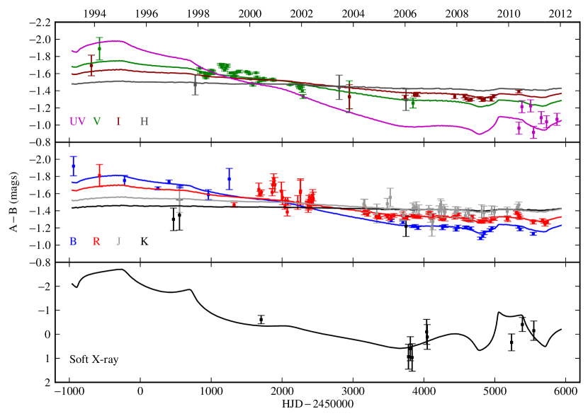
Figure 1.— Time delay-corrected difference in magnitudes between the A and B images of HE 1104 in each filter as a function of time (points with error bars). Some systematic errors have been added as described in Section 2. Curves show one of the best-fitting out of millions of microlensing light curves found by our simulation. The soft X-ray light curve is in its own panel because of its much larger range. The hard X-ray data are nearly identical, and we do not show them.

Our $B$-band data includes flux from the redshifted Ly$\alpha$ emission line, and $R$, $H$, and $K$ are also somewhat affected by the Ciii], H$\beta$, and H$\alpha$ lines, respectively. But in these broad filters, the line flux only amounts to a few percent of the total flux, and we do not expect it to have a strong effect on the microlensing results (Dai et al., 2010).

The light curve of the magnitude difference of the two quasar images, with error bars as described in this section, is shown for each band in Figure 1, together with an example of one of the many microlensing light curves that we fit to the data. Since this is the flux ratio of the two quasar images, and is corrected for the time delay, the variability is due to microlensing. The trend of increasing microlensing variability with decreasing wavelength, which is qualitatively expected for an accretion disk, can be easily seen.

2.2. UV Data

We have observed HE 1104 in the F275W filter (rest-frame $0.083$ $\mu$m) using the UVIS channel of the Wide Field Camera 3 aboard HST at 10 epochs roughly evenly spaced between 2009 December 4 and 2011 November 11. At each epoch, we combine four images totalling 2524 seconds of exposure time using the Multidrizzle task within the PyRAF software package. We take care to prevent the automatic cosmic ray rejection from masking out the PSF cores of the quasar components or bright comparison stars, manually removing some pixels from the bad pixel mask before repeating the final drizzle. The resulting images are clean and contain little besides the two quasar images and a handful of other pointlike objects.

We use aperture photometry to determine the fluxes of the quasar images and three other comparison objects. This is a very simple process because of the paucity of sources and relatively large separation between the quasar images. We use a square $1\farcs{}6$ aperture, and measure the sky background in a square annulus just outside the aperture, with an outer diameter twice that of the aperture. We then use the header keywords PHOTFLAM and PHOTZPT to convert the instrumental magnitudes to the ST system (in this filter, the offset from ST to AB magnitudes is $m_{\mathrm{AB}}-m_{\mathrm{ST}}=1.532$). Table 2 lists the ST magnitudes and formal uncertainties of quasar images A and B, as well as three comparison objects that we label a, b, and c. The first two of these, a and b, are the bright stars northeast of the lens labeled 4 and 3 (respectively) by Wisotzki et al. (1995), and the last is located at a position $(\Delta\alpha\cos\delta,\Delta\delta)=(-55\farcs{}7,-38\farcs{}2)$ relative to quasar image A. Objects a and b show little variability, while object c varies by $\sim$$0.3$ mags and may well be a quasar.

Since HE 1104 has a relatively high redshift, these UV observations probe the far-UV region of the quasar spectrum between the Lyman limit and the Ly$\beta$ emission line, from $\lambda\simeq 76$ to 91 Å in the rest frame. Though there may be some contamination from the remainder of the Lyman series, this is unlikely to be strong, and we consider the majority of the UV flux to be coming from the quasar accretion disk.

We shift the light curve of image B and use linear interpolation to estimate its delay-corrected light curve, resulting in a 7-epoch light curve. We add 0.05 mags in quadrature to the uncertainties of each image to account for the systematics introduced by this process. Fortunately, the mismatch between each measurement of image A and the nearest shifted measurement of B is usually fairly small, on the order of 10-30 days. The UV flux ratios are shown in the top panel of Figure 1.

2.3. X-Ray data

For our investigation of the X-ray properties of the quasar, we use the X-ray light curves of HE 1104 from Chen et al. (2012b) and Chartas et al. (2009). These data consist of soft-band (0.4$-$1.2 keV) and hard-band (1.2$-$8 keV) absorption-corrected count rates at nine epochs. We convert the count rates to instrumental magnitudes and symmetrize the resulting error bars by taking the geometric mean of the upper and lower errors.

The sampling of the X-ray light curves is generally not well-matched to the time delay between the two quasar images. In particular, the first epoch is separated from the rest by a period much longer than the delay. For this epoch we do not apply any delay correction, but simply augment the error bars in quadrature by 0.078 mags as previously described. For the remaining epochs we linearly interpolate the light curve of image B, then add the same extra uncertainty, except for the last two epochs. For these epochs, the observational cadence is within 10 days of the time delay, so that we can easily match one observation of B with the next observation of A. We add only half the extra uncertainty (0.039 mags) in these cases. The resulting soft-band X-ray flux ratios are shown in the bottom panel of Figure 1.

Unlike some other lensed quasars such as Q 2237$+$0305 (Chen et al., 2011) and RX J1131$-$1231 (Chartas et al., 2012), HE 1104 does not show significant differences between its hard and soft X-ray light curves. This immediately indicates that our microlensing simulation analysis will not be able to give definitive evidence of a difference in source size for these two bands. However, we ought to be able to place upper limits on the magnitude of the logarithm of their size ratio, which is an interesting result in its own right.

3. Microlensing Simulations

We model the gravitational microlensing of the two quasar images using the Bayesian Monte Carlo technique described by Kochanek (2004) and updated by Poindexter & Kochanek (2010a, b). This method uses ray-tracing to generate magnification patterns that encode the microlensing magnification experienced by each quasar image on top of its magnification from the “macro”-lensing by the lens galaxy as a whole. We generate new patterns for each epoch in the quasar’s light curve, allowing the stars to move between epochs. This causes the pattern of high-magnification caustics and low-magnification troughs to evolve. Together with the bulk relative motion of the quasar and the lens galaxy, this leads to variability in the microlensing magnifications. This work is the first to simultaneously fit observations at a variety of wavelengths and include the effects of stellar motions.

To generate the magnification patterns, we scatter stars randomly across a portion of the image plane. The mass function that we use for the microlens stars is a power law with a slope $d\ln N/d\ln M=-1.3$ and a mass range $M_{\mathrm{max}}/M_{\mathrm{min}}=50$. We vary the mean mass $\langle M\rangle$ between $0.03M_{\odot}$ and $10M_{\odot}$ in six logarithmically spaced steps. At the location of each quasar image, the fraction of the surface mass density made up of stars (as opposed to smoothly distributed dark matter) is determined from a global parameter, $f_{M/L}$. This parameter varies between 0 (no stars) and 1 (all stars), and specifies the amplitude of the stellar component (in a lensing model consisting of a de Vaucouleurs stellar component and a Navarro-Frenk-White dark matter component) relative to the best-fitting model with only stars. These models come from the work of Poindexter et al. (2007), and are constrained not only by the relative positions of the quasar images and lens galaxy, but by the images’ near-IR fluxes, which are not strongly affected by microlensing, and by their estimate of the lensing time delay. They find that a value of $f_{M/L}=0.3$ is most likely; this estimate would probably not change much if more recent time delay estimates were used instead. In the interest of fair sampling, we allow $f_{M/L}$ to take the values 0.1, 0.3, and 1.0. From these same lens models we obtain the total lensing convergence $\kappa_{\mathrm{tot}}$ and shear $\gamma$ at the positions of the quasar images, which together with $\langle M\rangle$ and $f_{M/L}$ determine the overall character of the magnification patterns. We set the rest-frame one-dimensional velocity dispersion of the stars to 301 km s^-1; this is calculated from the monopole strength of a singular isothermal sphere plus external shear (SIS$\gamma$) model for the lens potential. This has been shown to be a good estimator for the stellar velocity dispersion (Treu et al., 2006).

The effect of the quasar’s finite size is simulated by convolving the magnification patterns with a source light profile. We use a profile with surface brightness $I(r)\propto[\exp[(r/r_{\lambda})^{3/4}]-1]^{-1}$, where $r_{\lambda}$ is defined by the relation $kT_{\mathrm{eff}}(r_{\lambda})=h_{p}c/\lambda$. In standard thin disk theory,

$$r_{\lambda} =\left(\frac{45G\lambda^{4}M_{\mathrm{BH}}\dot{M}}{16\pi^{6}h_{p}c^{2}}\right)^{1/3}$$

$$=\left(9.7\times 10^{15}\,\mathrm{cm}\right)\left(\frac{\lambda}{\mu\mathrm{m}}\right)^{4/3}\left(\frac{M_{\mathrm{BH}}}{10^{9}M_{\odot}}\right)^{2/3}\left(\frac{L}{\eta L_{\mathrm{Edd}}}\right)^{1/3}~{},$$ (1)

where $\lambda$ is the rest wavelength, $L_{\mathrm{Edd}}$ is the Eddington luminosity, and $\eta$ is the radiative efficiency. In this model, the disk is a multicolor blackbody with temperature $T_{\mathrm{eff}}\propto r^{-\beta}$ and $\beta=3/4$. We neglect the effects of the inner edge of the disk. We vary the projected area of the disk at a fixed wavelength corresponding to the observed-frame $R$ band, allowing it to take values separated by 0.2 dex. We present most of our results, however, in terms of the half-light radius of the disk $r_{1/2}$, which is proportional to the square root of the area divided by the cosine of the inclination angle, and is equal to $2.44r_{\lambda}$ when $\beta=3/4$. The half-light radius is assumed to vary as a power law with wavelength, $r_{1/2}\propto\lambda^{\xi}$, and we allow its power-law slope $\xi$ to vary as well. Generically, $\xi$ is the reciprocal of the temperature slope, so for a thin disk its value is $4/3$. We allow it to take values ranging from $-1$ to $+2$ in 7 steps. Allowing the slope to vary is inconsistent with our choice of $\beta=3/4$ for the light profile of the source, but fortunately the details of the light profile, apart from the half-light radius, do not have a strong effect on the microlensing (Mortonson et al., 2005). Since the X-ray flux does not arise from the same blackbody source as the UV/optical flux, we do not assume that the X-ray size lies on the same power-law curve, instead allowing the area of the source in soft and hard X-rays to vary independently. We do this by pursuing an iterative strategy, first performing an initial simulation that is ignorant of the X-ray data, and then following up with secondary simulations for soft and hard X-ray data, each of which makes use of the output of the preceding simulation. The secondary simulations do not generate random trajectories for the quasar across the magnification patterns; instead they use the trajectories that successfully fit the data in the previous simulation, and they only vary a single new parameter: the area of the X-ray source. We do not take into account the lensing of the X-ray flux by the black hole, though given the compactness of the X-ray source it may be advisable to include this effect in future work (Chen et al., 2012a).

We vary the inclination of the accretion disk between $\cos i=1$ (face-on) and $\cos i=0.2$ (nearly edge-on) in 5 steps evenly distributed in $\cos i$; this is equivalent to a uniform prior on the orientation of the disk in three dimensions. Since an inclined disk looks like an ellipse to the observer, we also let the position angle of the projected disk take 9 values evenly distributed between $\phi_{a}=0^{\circ}$ (major axis aligned with north) and $\phi_{a}=160^{\circ}$ (rotated east of north). These parameters have subtle effects on the smoothed magnification patterns, and Poindexter & Kochanek (2010a) show that with moving patterns it is possible to constrain their values. But we note that they are helped by the relative importance of the random stellar motions in the lens system they consider (Q 2237), and the only other attempt to use this method so far does not obtain strong constraints on these parameters for the lens HE 0435$-$1223 (Blackburne et al., 2011a).

As described by Kochanek (2004) and Poindexter & Kochanek (2010a, b), this analysis method generates billions of trial paths that the quasar may take across the magnification patterns, and evaluates the likelihood of each trial based on the goodness of fit of the resulting light curve. The calculations are described in Equations (4) and (5) of Blackburne et al. (2011a); we set the “rescale” parameter $f_{0}^{2}$ to 2.0, 1.0, and 1.0 for the UV/optical, soft X-ray, and hard X-ray bands, respectively. Since each trial is associated with some location in parameter space, this Monte Carlo sampling gives us a reasonable idea of the joint likelihood function of our parameters. We then multiply the likelihood by our priors to obtain a Bayesian posterior probability density functions (PDFs) for our parameters. Our priors are mostly uniform, either in linear or logarithmic space. The mean microlens mass $\langle M\rangle$ and the variable parameterizing the fraction of the surface density in stars $f_{M/L}$ have logarithmic priors, and the inclination $\cos i$, the disk position angle $\phi_{a}$, and the wavelength slope $\xi=d\ln r_{1/2}/d\ln\lambda$ have linear priors. For the half-light radius $r_{1/2}$ itself we use both linear and logarithmic priors, because they can both be sensibly applied (see discussion by Blackburne et al., 2011a), and in order to evaluate the robustness of our results to changes in this prior. For the starting positions of the quasar on the magnification patterns we choose a simple uniform prior, and for its velocity we choose a circular Gaussian. The velocity prior is calculated in the manner described by Blackburne et al. (2011a), centering the Gaussian on the projection onto the lens plane of the velocity of the solar system relative to the cosmic microwave background (CMB), and setting its width to the quadrature sum of estimates of the peculiar velocities of the lens galaxy and the source galaxy. All velocities are corrected for cosmological time-dilation, and are converted to angular velocities using the angular diameter distances $D_{\mathrm{OL}}$, $D_{\mathrm{OS}}$, and $D_{\mathrm{LS}}$ (observer to lens, observer to source, and lens to source, respectively). Projected into the lens plane, the effective one-dimensional width of the velocity prior is

$$\sigma_{\mathrm{eff}}^{2}=\sigma_{L}^{2}+\sigma_{S}^{2}\left(\frac{1+z_{L}}{1+z_{S}}\right)^{2}\left(\frac{D_{\mathrm{OL}}}{D_{\mathrm{OS}}}\right)^{2}~{}.$$ (2)

We use the prescription cited by Mosquera & Kochanek (2011) for the estimates of the peculiar velocity dispersion, and find $\sigma_{L}=275$ km s^-1 and $\sigma_{S}=201$ km s^-1, yielding a width for the velocity prior of $\sigma_{\mathrm{eff}}=290$ km s^-1. This value is also approximately the typical speed of the quasar across the pattern.

4. Results

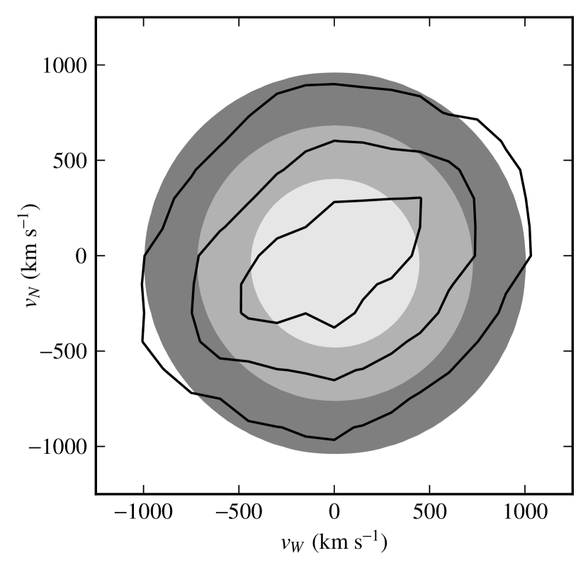
Figure 2.— Filled contours indicate the 68%, 95%, and 99% confidence levels of the velocity prior described in Section 3. Open contours show the posterior probability distribution of the transverse lens velocity (relative to that of the source and the observer). The direction of motion of the lens galaxy is $120\pm 40$ degrees, with a 180-degree degeneracy due to the symmetry of the elliptical disk model.

The product of the likelihood distribution with our priors gives a joint posterior probability distribution for our parameters. In this section, we examine the projections of this distribution, specifically the posterior PDFs for the velocity of the quasar relative to the lens galaxy, the inclination of the accretion disk and the position angle of its major axis, the mean mass of the stars causing the microlensing, the half-light radius of the quasar in the optical, soft X-ray, and hard X-ray bands, and the power-law slope of the half-light radius of the accretion disk with wavelength.

4.1. Velocity

The moving magnification patterns break the strict degeneracy between the velocity of the quasar relative to the lens and the mean mass of the stars, and allows us to put some actual constraints on the velocity. The posterior PDF for the transverse velocity of the lens (relative to the observer and source) is shown, together with our prior on the same quantity, in Figure 2. More precisely, this quantity is the angular velocity of the source across the magnification pattern, multiplied by the lens distance $D_{\mathrm{OL}}$ and time-dilated to the lens redshift, with a change of sign to make it a lens velocity rather than a source velocity. This differs somewhat in magnitude from the transverse peculiar velocity of the lens galaxy because it includes terms from the source and observer motions, but the lens term dominates and the difference is therefore small. Though the radial profile of the probability distribution is mostly determined by the prior, we do see a preference for a direction of motion of roughly $120\pm 40$ degrees (68% confidence), with a 180-degree degeneracy related to the bilateral symmetry of the (generally inclined) accretion disk.

4.2. Disk Inclination

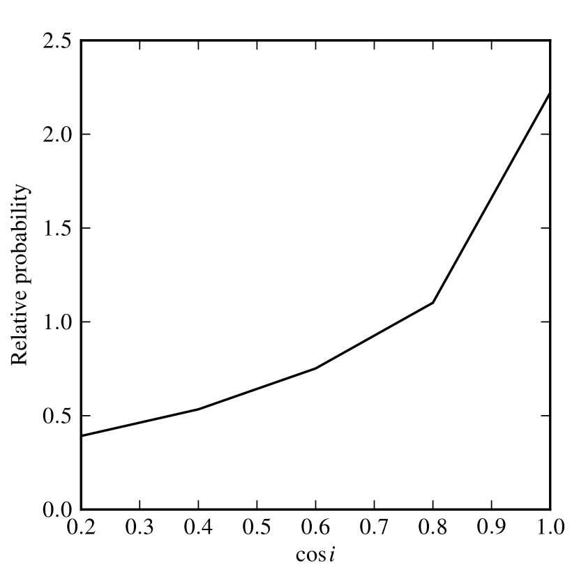
Figure 3.— Posterior distribution for the accretion disk inclination $\cos i$. A face-on disk has $\cos i=1$.

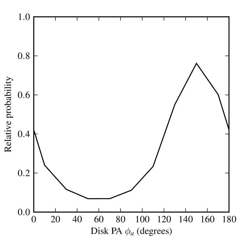
Figure 4.— Posterior distribution for the accretion disk major axis position angle $\phi_{a}$, measured in degrees East of North. Face-on ($\cos i=1$) solutions are excluded in calculating this result.

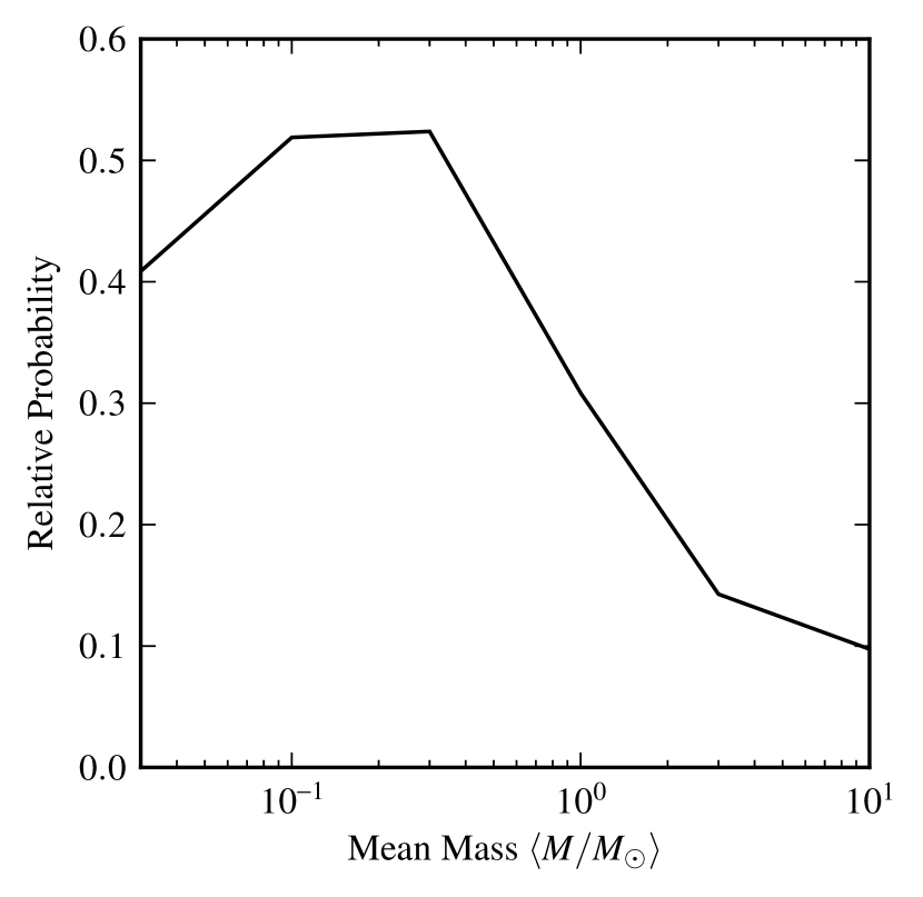
Figure 5.— Posterior distribution for the mean mass of the stars in the lensing galaxy.

The posterior PDFs for the accretion disk inclination $\cos i$ and the position angle of its major axis $\phi_{a}$ are shown in Figures 3 and 4. A face-on disk is favored, with $\cos i=1.0$ about four times as likely as $\cos i=0.5$. If we assume that the disk is in fact inclined and discard trials with $\cos i=1.0$, then its major-axis position angle is fairly well-determined, with a value of $150\pm 33$ degrees East of North (68% confidence).

4.3. Mean Microlens Mass

Figure 5 shows the posterior PDF for the mean mass $\langle M\rangle$ of the stellar microlenses. This quantity determines the scaling between the natural angular units of the magnification patterns (microlens Einstein radii) and units of physical length (e.g., cm) in the source plane. Even with our moving magnification patterns, it is still somewhat dependent on the velocity prior, in the sense that the very large transverse velocities suppressed by the Gaussian wings of our velocity prior correspond to very large mean masses. But we are confident in the appropriateness of this prior; in any case it seems quite unlikely that the mass function of stars in the lensing galaxy has a mean higher than 1 $M_{\odot}$. The distribution is fairly broad, and favors mean masses of 0.1 to 0.3 $M_{\odot}$.

4.4. Accretion Disk Size

The posterior PDFs for the deprojected half-light radius of the accretion disk in the $R$ band, and of the soft (0.4 to 1.2 keV) and hard (1.2 to 8 keV) X-ray emission regions are shown in Figure 6. The logarithm of the $R$-band radius (measured in cm) is $16.0^{{}_{+0.3}}_{{}^{-0.4}}$ with the logarithmic prior. With the linear prior, this value rises to $16.2\pm 0.3$. The X-ray PDFs do not converge at small sizes, as the finite resolution of the magnification patterns prevents us from going to smaller sizes, but the cutoff scale is smaller than the gravitational radius of the black hole (regardless of which black hole mass estimate is chosen). The three vertical lines in Figure 6 show the gravitational radius, the $R$-band radius estimated from the flux of the quasar, and the $R$-band radius predicted by the thin disk model, assuming an accretion efficiency $\eta=0.1$ and an Eddington fraction $L/L_{\mathrm{Edd}}=1$. All assume the H$\beta$ mass estimate of Assef et al. (2011). With the logarithmic prior the source is smaller than $\log(r_{1/2}/\mathrm{cm})=15.33$ at 95% confidence in both soft and hard X-rays. With the linear prior, the upper limits are 15.71 (soft) and 15.59 (hard). If the Peng et al. (2006) black hole mass estimate is correct, then half the X-ray light is originating within a radius less than about 6 (logarithmic prior) or 12-14 (linear prior) gravitational radii.

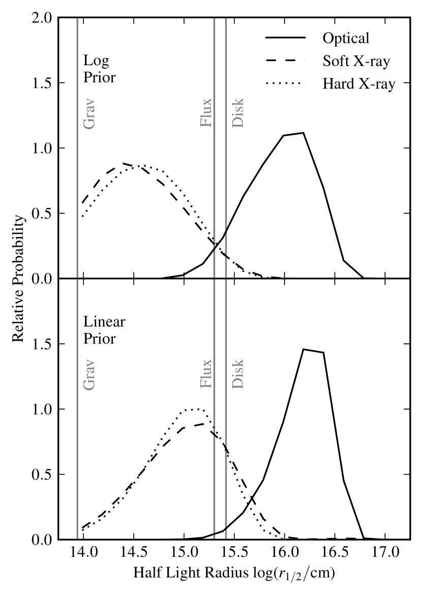
Figure 6.— Posterior distribution for the half-light radius of the quasar accretion disk in the $R$ band and the two X-ray bands. In the upper panel we use a logarithmic prior, and in the lower panel we use a linear prior. The stellar mean mass $\langle M/M_{\odot}\rangle$ is fixed at 0.3. The gravitational radius of the black hole and the $R$-band size estimates based on the quasar flux and the thin disk model are shown as a vertical lines, marked “Grav,” “Flux,” and “Disk” respectively. The “Grav” and “Disk” values assume the H$\beta$ black hole mass estimate of Assef et al. (2011), and can shift up to $\sim$0.5 dex based on the uncertainties or by using the H$\alpha$ or Civ estimates.

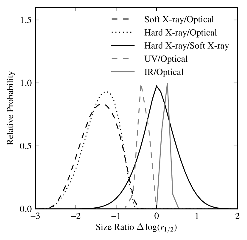
Figure 7.— Posterior distributions for the ratios of the quasar’s half-light radius. The black curves indicate ratios of the X-ray sizes; for these curves the mean mass $\langle M\rangle$ is set to $0.3M_{\odot}$. The X-ray emission is much more compact than the observed-frame $R$-band emission (labeled “Optical”). Also, our X-ray data rule out a very large difference in the sizes of the hard and soft X-ray sources. The gray curves indicate the size of the accretion disk at the (observed-frame) UV and $J$-band wavelengths, relative to the $R$-band size. Since we parameterize the disk using the $R$-band size and the wavelength slope $\xi$, the gray curves are simply scaled versions of the posterior distribution for $\xi$ (see Figure 8).

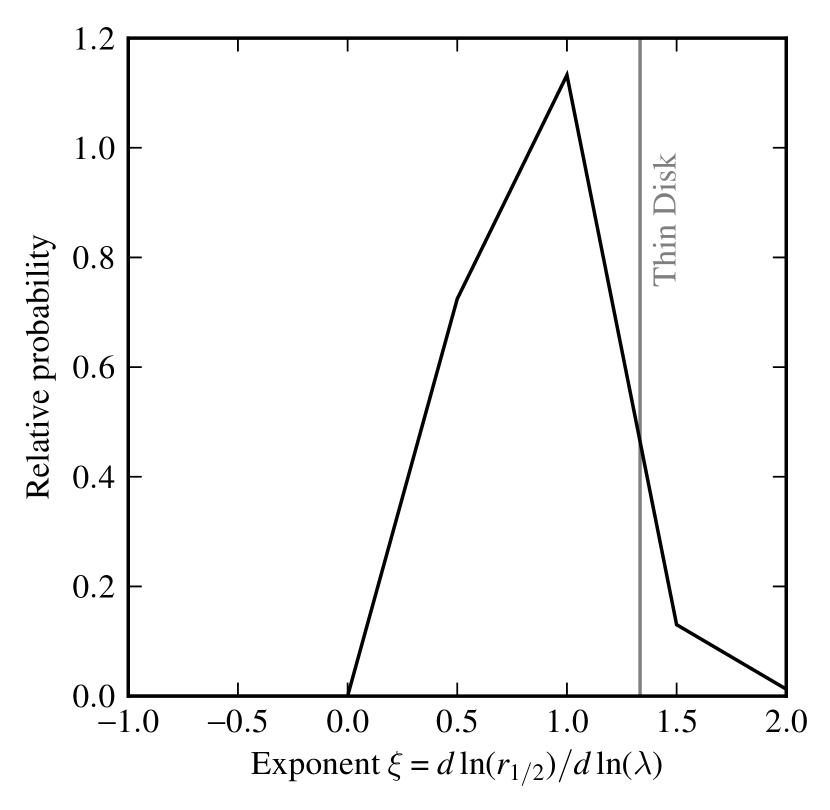
Figure 8.— Posterior probability distribution for the power-law slope of the wavelength dependence of the half-light radius. The standard thin disk model predicts a value of 4/3 since $T_{\mathrm{eff}}\propto r^{-3/4}$.

The deprojected half-light radii are calculated from the projected area of the source $A=\pi(r_{1/2}/2.44)^{2}\cos i$. With the logarithmic (linear) prior, we find that $\log(A/\mathrm{cm}^{2})=31.54^{{}_{+0.64}}_{{}^{-0.72}}$ ($32.26^{{}_{+0.39}}_{{}^{-0.50}}$). Likewise, the 95% confidence upper limit on the logarithm of the source area is 30.23 (31.34) for soft X-rays, and 30.20 (31.11) for hard X-rays. These projected areas are more appropriate for comparison with previous work that does not vary the inclination of the source, but since HE 1104 seems to have a relatively face-on disk, this correction is not very important.

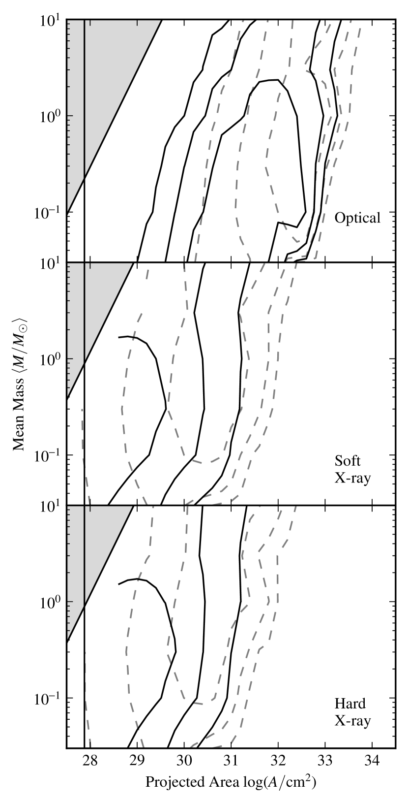
Figure 9.— Joint posterior probability distribution for the mean microlens mass $\langle M\rangle$ and the projected source area $A$ in the $R$ band (top panel), soft X-rays (middle panel), and hard X-rays (bottom panel). The solid black (dashed gray) curves indicate a logarithmic (linear) prior on the area. The vertical line indicates the square of the black hole’s gravitational radius, as calculated using the black hole mass estimate of Assef et al. (2011). The gray region cannot be sampled because of the finite resolution of the magnification patterns.

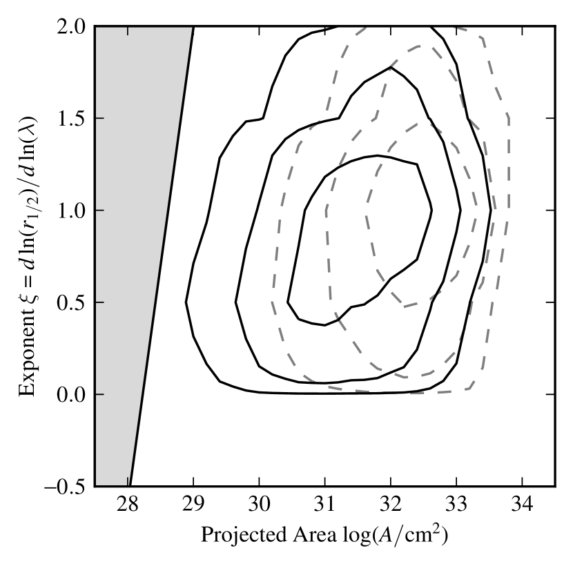
Figure 10.— Joint posterior probability distribution for the exponent $\xi$ and the projected $R$-band source area $A$. The solid black (dashed gray) curves indicate a logarithmic (linear) prior on the area. The gray area is excluded because the observed-frame UV disk would be smaller than the resolution of the magnification patterns.

The soft and hard X-ray half-light radii PDFs are nearly identical, which is consistent with our expectations given the similarity of their light curves. To investigate the question of which is larger, we show in Figure 7 the posterior PDFs for the logarithm of the ratios between the sizes in the various bands. The solid curve indicates the ratio of the hard band size to the soft band size. It peaks fairly sharply near zero, indicating a ratio of unity. The symmetric tails on either side mean that we cannot with our current data distinguish which is the larger, but we can say that their sizes do not differ too much: at 68% confidence the logarithm of the ratio falls between $-0.45$ and $+0.46$. Figure 7 also indicates that the X-ray sizes are much smaller than the $R$-band sizes, with $\Delta\log(r_{1/2})=-1.40^{{}_{+0.44}}_{{}^{-0.48}}$ for the soft band and $-1.35^{{}_{+0.38}}_{{}^{-0.46}}$ in the hard band (68% confidence). These constraints are tighter than the previous figure would imply, due to covariances between the optical and X-ray sizes that are not apparent in Figure 6.

Figure 8 shows the posterior PDF for the power-law slope of the wavelength dependence of the half-light radius, a quantity we call $\xi$. For an accretion disk that radiates as a multi-temperature blackbody, this exponent is the reciprocal of the power-law slope $\beta$ of the temperature profile $T_{\mathrm{eff}}(r)\propto r^{-\beta}$. So for the standard thin disk model, we expect $\xi=d\log r_{1/2}/d\log\lambda=\beta^{-1}=4/3$ (neglecting the effect of the inner disk edge, as is reasonable to do at radii of many $r_{g}$). Our probability distribution peaks at a value of 1.0, with a median value of 0.84, and with 68% of the probability lying between values of 0.44 and 1.30. This is consistent with the thin disk value, though it is interesting that the majority of the probability lies toward smaller values of $\xi$, or (equivalently) steeper temperature profiles. Using this posterior distribution, we show in Figure 7 the logarithm of the size ratio between the observed-frame UV and $R$-band disks, and between the $J$-band and $R$-band disks. These are just scaled versions of the distribution in Figure 8.

Figures 6 and 7 and the source size estimates quoted in this section are produced with the mean microlens mass $\langle M\rangle$ fixed at its most likely value of $0.3\,M_{\odot}$. We do this rather than marginalizing over $\langle M\rangle$ in order to avoid an artificial decrease in the probability of small source sizes due to the finite resolution of the magnification patterns. This artificial decrease happens because there is no contribution to the probability of small sizes from trials with large $\langle M\rangle$ (and thus with a projected pixel size larger than the area of the source). To explore the effect of this choice, we show in Figure 9 the joint posterior PDF for the mean mass $\langle M\rangle$ and the projected source area $A=\pi(r_{1/2}/2.44)^{2}\cos i$. Some covariance between these parameters can be seen; this is expected because the area is measured in units of the square of the microlens Einstien radius. The figure also shows the resolution limit of the magnification patterns, and it is clear that the $R$-band source is well-resolved in all cases, but that the X-ray sources are not much larger than the pixels in the magnification patterns (despite the higher-resolution patterns we use in these simulations).

Another concern for the accretion disk simulations is that at large values of $\xi$ the HST UV observations (i.e., the bluest apart from X-rays) will probe source sizes small enough to be unresolved, even though the source is resolved in the $R$ band. Figure 10 shows the joint posterior PDF of the exponent $\xi$ and the $R$-band projected source area $A$. We also show the region where the UV source is unresolved, with $\langle M\rangle=0.3M_{\odot}$. The probability distribution clearly converges at small areas, so this concern is unfounded.

5. Discussion and Conclusions

HE 1104 is the third lensed quasar to be analyzed using dynamic microlensing magnification patterns, after Q 2237 (Poindexter & Kochanek, 2010a, b; Mosquera et al., 2013) and HE 0435$-$1223 (Blackburne et al., 2011a). The inclusion of the random motions of the stars allows us to constrain the inclination of the accretion disk, the position angle of its projected major axis, and the direction of the lens galaxy’s motion relative to the quasar. In this case, the data favor a low disk inclination, with $\cos i=1.0$ about four times as likely as $\cos i=0.5$ (see Figure 3). This is similar to the result that Poindexter & Kochanek (2010a) find for Q 2237, and supports the “unification” model for AGNs, which predicts that bright Type 1 quasars such as these have a low inclination. For models with a nonzero inclination, we find that the major axis of HE 1104’s projected disk is about $150\pm 33$ degrees east of north (see Figure 4. We also find that the lens galaxy’s motion is likely toward the northwest or southeast, with a most likely angle of 120 degrees east of north (or 30 degrees west of north), and with 68% confidence error bars of 40 degrees. The magnitude of the velocity is unfortunately not robustly constrained, and depends on our velocity prior (see Section 3 and Figure 2).

We also produce a posterior PDF for the mean mass of the stars in the lensing galaxy (see Figure 5). The distribution peaks between $0.1$ and $0.3\,M_{\odot}$, which is consistent with what is observed in other lens galaxies (Poindexter & Kochanek, 2010b; Blackburne et al., 2011a) and in the Milky Way (Holtzman et al., 1998; Zoccali et al., 2000). Our distribution implies a slightly higher mean mass than that of Chartas et al. (2009), which is probably due to differences in the velocity priors. Their analysis uses static magnification patterns, and (probably more importantly) their peculiar velocities are smaller than the ones that we have chosen, which would tend to make their mean mass estimates smaller.

Our results for the half-light radius of the accretion disk in the observer-frame $R$ band ($0.2\,\mu$m in the rest frame) agree with those of previous studies of HE 1104 (Poindexter et al., 2008; Morgan et al., 2008; Chartas et al., 2009). Like these studies, we find that HE 1104, like several other lensed quasars, has an accretion disk much larger than would be expected from either the thin disk model or the quasar flux (see Equations 2 and 3 of Poindexter et al. (2008)). These estimates, marked “Flux” and “Disk” respectively, are plotted for the observed-frame $R$ band in Figure 6. Poindexter et al. (2008) suggest a small value for the accretion disk temperature profile slope $\beta$ as a possible solution to the discrepancy between the microlensing size and the flux size, supported by their estimated value of $\beta=0.61^{{}_{+0.21}}_{{}^{-0.17}}$, smaller than the canonical 0.75. But our result for the slope of the size-wavelength relation, $\xi=\beta^{-1}=1.0^{{}_{+0.30}}_{{}^{-0.46}}$, implies a range of 0.77 to 1.85 for $\beta$. This is roughly consistent with the Poindexter et al. (2008) result, but some tension remains. It seems that our new data indicate that the area of the disk changes less with wavelength than was previously thought. Indeed, our value favors a temperature profile steeper than the standard thin disk model. This would only serve to exacerbate the flux size discrepancy (see Morgan et al., 2010). Multiwavelength observations of more lensed quasars will shed more light on this ongoing mystery.

Our upper limits on the size of quasar at X-ray wavelengths are quite strong. It is clear that the majority of the hard and soft X-ray flux is coming from the innermost $\sim$30 $r_{g}$, assuming the H$\beta$-based black hole mass estimate of Assef et al. (2011). This result is comparable to the upper limit that Chartas et al. (2009) find using a single X-ray data point. This lack of improvement is partly due to our practice of dividing the X-ray flux into two bands and of marginalizing over a variety of source inclinations (both of which broaden the posterior PDF), and partly due to the fact that we have not yet been able to sample the X-ray light curve on time scales smaller than the source crossing time (see Mosquera & Kochanek, 2011). For HE 1104 the soft and hard X-ray data are very similar, and so we are unable to determine which band has a larger size, though we do conclude that their sizes do not differ by more than 0.46 dex. This result is similar to those of Blackburne et al. (2011a) for HE 0435 and Morgan et al. (2012) for Q J0158$-$4325. The question of the two X-ray bands’ relative sizes is quite interesting, since it can address the corona/reflection model. If the direct component of the emission dominates, the hard band, coming from a hotter electron population, ought to be smaller. But a prominent reflection from the accretion disk could reverse this result, since the reflected spectrum is harder than the input spectrum, and may well be more extended. Recent papers presenting X-ray observations have used simple microlensing models to address this question (Chartas et al., 2012; Chen et al., 2012b), but full microlensing simulations are needed to put rigorous constraints on the sizes. Some of the X-ray data display fairly strong chromatic variation, so interesting results should be forthcoming.

References

- Anguita et al. (2008) Anguita, T., Schmidt, R. W., Turner, E. L., Wambsganss, J., Webster, R. L., Loomis, K. A., Long, D., & McMillan, R. 2008, A&A, 480, 327
- Assef et al. (2011) Assef, R. J., et al. 2011, ApJ, 742, 93
- Bate et al. (2008) Bate, N. F., Floyd, D. J. E., Webster, R. L., & Wyithe, J. S. B. 2008, MNRAS, 391, 1955
- Blackburne & Kochanek (2010) Blackburne, J. A., & Kochanek, C. S. 2010, ApJ, 718, 1079
- Blackburne et al. (2011a) Blackburne, J. A., Kochanek, C. S., Chen, B., Dai, X., & Chartas, G. 2011a, arXiv:1112.0027
- Blackburne et al. (2011b) Blackburne, J. A., Pooley, D., Rappaport, S., & Schechter, P. L. 2011b, ApJ, 729, 34
- Blaes et al. (2001) Blaes, O., Hubeny, I., Agol, E., & Krolik, J. H. 2001, ApJ, 563, 560
- Chartas et al. (2012) Chartas, G., Kochanek, C. S., Dai, X., Moore, D., Mosquera, A. M., & Blackburne, J. A. 2012, ApJ, 757, 137
- Chartas et al. (2009) Chartas, G., Kochanek, C. S., Dai, X., Poindexter, S., & Garmire, G. 2009, ApJ, 693, 174
- Chen et al. (2012a) Chen, B., Dai, X., Baron, E., & Kantowski, R. 2012a, arXiv:1211.6487
- Chen et al. (2011) Chen, B., Dai, X., Kochanek, C. S., Chartas, G., Blackburne, J. A., & Kozłowski, S. 2011, ApJ, 740, L34
- Chen et al. (2012b) Chen, B., Dai, X., Kochanek, C. S., Chartas, G., Blackburne, J. A., & Morgan, C. W. 2012b, ApJ, 755, 24
- Courbin et al. (1998) Courbin, F., Lidman, C., & Magain, P. 1998, A&A, 330, 57
- Dai et al. (2010) Dai, X., Kochanek, C. S., Chartas, G., Kozłowski, S., Morgan, C. W., Garmire, G., & Agol, E. 2010, ApJ, 709, 278
- DePoy et al. (2003) DePoy, D. L., et al. 2003, in Society of Photo-Optical Instrumentation Engineers (SPIE) Conference Series, Vol. 4841, Society of Photo-Optical Instrumentation Engineers (SPIE) Conference Series, ed. M. Iye & A. F. M. Moorwood, 827–838
- Dexter & Agol (2011) Dexter, J., & Agol, E. 2011, ApJ, 727, L24
- Eigenbrod et al. (2008) Eigenbrod, A., Courbin, F., Meylan, G., Agol, E., Anguita, T., Schmidt, R. W., & Wambsganss, J. 2008, A&A, 490, 933
- Fabian et al. (1989) Fabian, A. C., Rees, M. J., Stella, L., & White, N. E. 1989, MNRAS, 238, 729
- Floyd et al. (2009) Floyd, D. J. E., Bate, N. F., & Webster, R. L. 2009, MNRAS, 398, 233
- Gil-Merino et al. (2002) Gil-Merino, R., Wisotzki, L., & Wambsganss, J. 2002, A&A, 381, 428
- Greene et al. (2010) Greene, J. E., Peng, C. Y., & Ludwig, R. R. 2010, ApJ, 709, 937
- Hainline et al. (2012) Hainline, L. J., et al. 2012, ApJ, 744, 104
- Holtzman et al. (1998) Holtzman, J. A., Watson, A. M., Baum, W. A., Grillmair, C. J., Groth, E. J., Light, R. M., Lynds, R., & O’Neil, Jr., E. J. 1998, AJ, 115, 1946
- Jiménez-Vicente et al. (2012) Jiménez-Vicente, J., Mediavilla, E., Muñoz, J. A., & Kochanek, C. S. 2012, ApJ, 751, 106
- Kochanek (2004) Kochanek, C. S. 2004, ApJ, 605, 58
- Kochanek et al. (2006) Kochanek, C. S., Morgan, N. D., Falco, E. E., McLeod, B. A., Winn, J. N., Dembicky, J., & Ketzeback, B. 2006, ApJ, 640, 47
- Laor (1991) Laor, A. 1991, ApJ, 376, 90
- Lehár et al. (2000) Lehár, J., et al. 2000, ApJ, 536, 584
- McClintock et al. (2011) McClintock, J. E., et al. 2011, Classical and Quantum Gravity, 28, 114009
- Morgan et al. (2008) Morgan, C. W., Eyler, M. E., Kochanek, C. S., Morgan, N. D., Falco, E. E., Vuissoz, C., Courbin, F., & Meylan, G. 2008, ApJ, 676, 80
- Morgan et al. (2010) Morgan, C. W., Kochanek, C. S., Morgan, N. D., & Falco, E. E. 2010, ApJ, 712, 1129
- Morgan et al. (2012) Morgan, C. W., et al. 2012, ApJ, 756, 52
- Mortonson et al. (2005) Mortonson, M. J., Schechter, P. L., & Wambsganss, J. 2005, ApJ, 628, 594
- Mosquera & Kochanek (2011) Mosquera, A. M., & Kochanek, C. S. 2011, ApJ, 738, 96
- Mosquera et al. (2013) Mosquera, A. M., Kochanek, C. S., Chen, B., Dai, X., Blackburne, J. A., & Chartas, G. 2013, arXiv:1301.5009
- Mosquera et al. (2011) Mosquera, A. M., Muñoz, J. A., Mediavilla, E., & Kochanek, C. S. 2011, ApJ, 728, 145
- Muñoz et al. (2011) Muñoz, J. A., Mediavilla, E., Kochanek, C. S., Falco, E. E., & Mosquera, A. M. 2011, ApJ, 742, 67
- Novikov & Thorne (1973) Novikov, I. D., & Thorne, K. S. 1973, in Black Holes (Les Astres Occlus), ed. C. Dewitt & B. S. Dewitt, 343–450
- Ofek & Maoz (2003) Ofek, E. O., & Maoz, D. 2003, ApJ, 594, 101
- Peng et al. (2006) Peng, C. Y., Impey, C. D., Rix, H.-W., Kochanek, C. S., Keeton, C. R., Falco, E. E., Lehár, J., & McLeod, B. A. 2006, ApJ, 649, 616
- Poindexter & Kochanek (2010a) Poindexter, S., & Kochanek, C. S. 2010a, ApJ, 712, 668
- Poindexter & Kochanek (2010b) —. 2010b, ApJ, 712, 658
- Poindexter et al. (2008) Poindexter, S., Morgan, N., & Kochanek, C. S. 2008, ApJ, 673, 34
- Poindexter et al. (2007) Poindexter, S., Morgan, N., Kochanek, C. S., & Falco, E. E. 2007, ApJ, 660, 146
- Pooley et al. (2007) Pooley, D., Blackburne, J. A., Rappaport, S., & Schechter, P. L. 2007, ApJ, 661, 19
- Pooley et al. (2006) Pooley, D., Blackburne, J. A., Rappaport, S., Schechter, P. L., & Fong, W.-f. 2006, ApJ, 648, 67
- Remy et al. (1998) Remy, M., Claeskens, J.-F., Surdej, J., Hjorth, J., Refsdal, S., Wucknitz, O., Sorensen, A. N., & Grundahl, F. 1998, New A, 3, 379
- Reynolds & Nowak (2003) Reynolds, C. S., & Nowak, M. A. 2003, Phys. Rep., 377, 389
- Schechter et al. (2003) Schechter, P. L., et al. 2003, ApJ, 584, 657
- Shakura & Sunyaev (1973) Shakura, N. I., & Sunyaev, R. A. 1973, A&A, 24, 337
- Treu et al. (2006) Treu, T., Koopmans, L. V., Bolton, A. S., Burles, S., & Moustakas, L. A. 2006, ApJ, 640, 662
- Wisotzki et al. (1995) Wisotzki, L., Koehler, T., Ikonomou, M., & Reimers, D. 1995, A&A, 297, L59
- Wisotzki et al. (1993) Wisotzki, L., Koehler, T., Kayser, R., & Reimers, D. 1993, A&A, 278, L15
- Wyrzykowski et al. (2003) Wyrzykowski, L., et al. 2003, Acta Astron., 53, 229
- Zoccali et al. (2000) Zoccali, M., Cassisi, S., Frogel, J. A., Gould, A., Ortolani, S., Renzini, A., Rich, R. M., & Stephens, A. W. 2000, ApJ, 530, 418