Magnetic monopoles and synthetic spin-orbit coupling in Rydberg macrodimers

Abstract

We show that sizeable Abelian and non-Abelian gauge fields arise in the relative motion of two dipole-dipole interacting Rydberg atoms. Our system exhibits two magnetic monopoles for adiabatic motion in one internal two-atom state. These monopoles occur at a characteristic distance between the atoms that is of the order of one micron. The deflection of the relative motion due to the Lorentz force gives rise to a clear signature of the effective magnetic field. In addition, we consider non-adiabatic transitions between two near-degenerate internal states and show that the associated gauge fields are non-Abelian. We present quantum mechanical calculations of this synthetic spin-orbit coupling and show that it realizes a velocity-dependent beamsplitter.

Gauge theories represent a cornerstone of modern physics and play a prominent role in classical and quantum electrodynamics, the standard model of elementary particle physics and condensed matter physics. In view of the importance of this concept tremendous effort has been made to create artificial gauge fields for neutral atoms ruseckas:05 ; dalibard:11 ; dum:96 ; lin:09 ; lin:09n ; lin:11 ; aidelsburger:11 ; jaksch:03 ; struck:11 ; struck:12 ; jimenez_garcia:12 ; hauke:12 and to investigate the resulting atom dynamics in the quantum regime. In these schemes, engineered light-matter interactions cause neutral atoms to behave like charged particles in an electromagnetic field.

Artificial gauge fields allow the simulation of theoretical models that are otherwise inaccessible. For example, the realization of magnetic monopoles affecting the relative nuclear motion of diatomic molecules has been discussed in moody:86 . However, gauge field effects in molecules are usually very small since they arise from terms that are neglected in the Born-Oppenheimer approximation (BOA) born:27 which is very well satisfied in many molecular systems. In addition, the experimental observation of these effects is considerably hampered by the small size of conventional molecules.

Recently, extremely large molecules comprised of two Rydberg atoms with non-overlapping electron clouds have been proposed boisseau:02 ; samboy:11 ; kiffner:12 and observed overstreet:09 . Typical internuclear spacings exceed $1\,\mu\text{m}$, and thus the experimental observation of Rydberg-Rydberg correlations becomes feasible schwarzkopf:11 ; schauss:12 ; gaetan:09 ; urban:09 . These so-called macrodimers interact via well-understood and controllable dipole-dipole potentials. Importantly, the validity of the BOA cannot be established via the mass ratio of nuclei and electrons for these systems.

Here we show that dipole-dipole interacting Rydberg atoms can exhibit Abelian and non-Abelian gauge fields that influence the quantum dynamics of the relative atomic motion substantially. In contrast to the Rydberg macrodimer proposal in kiffner:12 , the system in Fig. 1 is distinguished by an asymmetric Stark shift of the Zeeman sublevels. We find that this broken symmetry gives rise to magnetic monopoles if the system evolves adiabatically in one internal two-atom state. These monopoles occur at a characteristic distance between the atoms that is of the order of one micron. The Lorentz force associated with the magnetic field near a monopole results in a sizeable deflection of the relative atomic motion. This effect can be interpreted in terms of an exchange between orbital and internal spin angular momentum as the internal molecular state changes while the atoms move. Moreover, we investigate non-adiabatic transitions between two internal two-atom states and find that the associated gauge fields are are non-Abelian. This synthetic spin-orbit coupling creates a coherent superposition of two spatial configurations of the atoms. We expect that our findings are relevant for other dipole-dipole interacting systems like polar molecules and magnetic atoms.

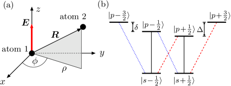
Figure 1: (Color online) (a) System geometry of two dipole-dipole interacting Rydberg atoms. $\boldsymbol{R}$ is the relative position of atom 2 with respect to atom 1, and $\rho$ is the distance of atom 2 from the $z$ axis. The $z$ direction is distinguished by a DC electric field $\boldsymbol{E}$. (b) Internal level structure of each Rydberg atom. The Stark shifts $\delta$ and $\Delta$ are negative. We assume $\delta\not=\Delta$. The dipole transitions indicated by blue dotted, black solid and red dashed lines couple to $\sigma^{-}$, $\pi$ and $\sigma^{+}$ polarized fields, respectively.

The geometry of the two atom system under consideration is shown in Fig. 1(a). In order to account for the azimuthal symmetry of the system, we express the relative position $\boldsymbol{R}$ of atom 2 with respect to atom 1 in terms of cylindrical coordinates, $\boldsymbol{R}=(\rho\cos\phi,\rho\sin\phi,z)$. We omit the center-of-mass motion which is uniform and investigate the relative motion of the two dipole-dipole interacting Rydberg atoms. The Hamiltonian of this system is given by

$$H=H_{\text{R}}+H_{\text{S}}+V_{\text{dd}},$$ (1)

where $H_{\text{R}}=\boldsymbol{p}^{2}/(2\mu)$ is the kinetic energy of the relative motion and $\mu$ is the reduced mass. $H_{\text{S}}$ describes the internal levels of the two uncoupled atoms and $V_{\text{dd}}$ is the dipole-dipole interaction  kiffner:12 . In each Rydberg atom we consider two angular momentum multiplets as shown in Fig. 1(b). The lower $ns_{1/2}$ states have total angular momentum $J=1/2$, and the excited multiplet is comprised of $np_{3/2}$ states with total angular momentum $J=3/2$. We specify the individual atomic states $|\ell m_{j}\rangle$ by their orbital angular momentum $\ell$ and azimuthal total angular momentum $m_{j}$. A DC electric field $\boldsymbol{E}$ in the $z$ direction defines the quantization axis and gives rise to Stark shifts of the magnetic sublevels. We assume that the Stark shifts are different in the $m_{j}>0$ and $m_{j}<0$ manifolds, which could be achieved, e.g., by inducing additional AC stark shifts. For simplicity we focus on the level scheme shown in Fig. 1(b), where the asymmetry is characterized by the ratio $\Delta/\delta$ of the Stark shifts $\delta$ and $\Delta$. The relevant subspace of two-atom states is spanned by the $N=16$ $nsnp$ states where one atom is in a $ns_{1/2}$ state and the other in a $np_{3/2}$ state. For every value of $\boldsymbol{R}$ we introduce a set of orthonormal eigenstates of the Hamiltonian $H_{\text{S}}+V_{\text{dd}}$,

$$(H_{\text{S}}+V_{\text{dd}})|\psi_{i}(\boldsymbol{R})\rangle=\epsilon_{i}(\boldsymbol{R})|\psi_{i}(\boldsymbol{R})\rangle,$$ (2)

where $\epsilon_{i}(\boldsymbol{R})$ are the corresponding eigenvalues. With these definitions, the full quantum state of the two-atom system can be written as $|\Psi\rangle=\sum_{i=1}^{N}\int\text{d}^{3}R\;\alpha_{i}(\boldsymbol{R})|\psi_{i}(\boldsymbol{R})\rangle\otimes|\boldsymbol{R}\rangle$. Next we assume that the dynamics is confined to $q$ eigenstates of $H_{\text{S}}+V_{\text{dd}}$, i.e., there may be non-adiabatic transitions within the first $q$ eigenstates, but transitions to other states $|\psi_{l}(\boldsymbol{R})\rangle$ ($l>q$) can be neglected. We follow the procedure described in wilczek:84 ; dum:96 ; ruseckas:05 ; dalibard:11 and derive from Eq. (1) an effective Schrödinger equation for the wavefunctions $\boldsymbol{\mathcal{\alpha}}=(\alpha_{1},\ldots,\alpha_{q})$, $q<N$,

$$i\hbar\partial_{t}\boldsymbol{\alpha}=\left[\frac{1}{2\mu}(\boldsymbol{p}-\boldsymbol{A})^{2}+V+\Phi\right]\boldsymbol{\alpha}.$$ (3)

Equation (3) is equivalent to the Schrödinger equation of a charged particle in an electromagnetic field, characterized by the vector potential $\boldsymbol{A}$ and scalar potential $\Phi$. Here $V$ and $\boldsymbol{A}$ are $q\times q$ matrices whose matrix elements for $k,l\leq q$ are given by

$$V_{kl}=\delta_{kl}\epsilon_{k}(\boldsymbol{R}),\quad\boldsymbol{A}_{kl}=i\hbar\langle\psi_{k}(\boldsymbol{R})|\nabla|\psi_{l}(\boldsymbol{R})\rangle,$$ (4)

and $\delta_{kl}$ is the Kronecker delta. We find that the impact of the scalar potential $\Phi$ on the presented results is negligible, and thus omit it in the following. The Cartesian components $B^{(i)}$ ($i\in\{1,2,3\}$) of the artificial magnetic field are defined as

$$B^{(i)} =\frac{1}{2}\varepsilon_{ikl}F^{(kl)},$$ (5)

$$F^{(kl)} =\partial_{k}A^{(l)}-\partial_{l}A^{(k)}-\frac{\imath}{\hbar}\left[A^{(k)},A^{(l)}\right],$$ (6)

where $\varepsilon_{ikl}$ is the Levi-Civita tensor and we employed Einstein’s sum convention. The $q\times q$ matrices $A^{(i)}$ describe non-Abelian gauge fields if the commutator $[A^{(k)},A^{(l)}]$ is different from zero. The magnetic field gives rise to a Lorentz force which is proportional to the velocity $\boldsymbol{v}=(\boldsymbol{p}-\boldsymbol{A})/\mu$ of the relative motion.

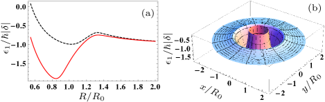
Figure 2: (Color online) (a) Potential curve $\epsilon_{1}$ in the $x-y$ plane as a function of scaled internuclear spacing $R/R_{0}$. The parameters are $\Delta=-1.5|\delta|$ (dashed black line) and $\Delta=-3|\delta|$ (red solid line). (b) Potential curve $\epsilon_{1}$ in the $x-y$ plane for $\Delta=-3|\delta|$.

The eigenstates $|\psi_{i}\rangle$ and eigenvalues $\epsilon_{i}$ of the Hamiltonian $H_{\text{S}}+V_{\text{dd}}$ in Eq. (2) can be obtained numerically. Here we focus on one particular potential curve that exhibits a potential well such that the two dipole-dipole interacting Rydberg atoms can form a giant molecule. This potential curve is labelled by $\epsilon_{1}$ and shown in Fig. 2(a) for different ratios of $\Delta/\delta$. The potential minimum occurs roughly at the characteristic length $R_{0}=(|\mathcal{D}|^{2}/(4\pi\epsilon_{0}\hbar|\delta|)^{1/3}$ denoting the distance where the magnitude of the dipole-dipole interaction equals the Stark splitting $\hbar|\delta|$  kiffner:12 , and $|\mathcal{D}|$ is the reduced dipole matrix element of the $ns\leftrightarrow np$ transition kiffner:12 . Due to the azimuthal symmetry of the system a donut shaped potential well arises in the $x-y$ plane [see Fig. 2(b)]. The dependence of $\epsilon_{1}$ on $x$ and $z$ is displayed in Fig. 3(a), showing that the width of the potential well in $z$ direction is comparable to its width in the $x-y$ plane. Note that a potential well with similar features but for $\delta=\Delta<0$ was reported in kiffner:12 .

Next we consider the case $q=1$ in Eq. (3) and consider the adiabatic motion in the eigenstate $|\psi_{1}\rangle$ corresponding to $\epsilon_{1}$. We choose the phase of $|\psi_{1}\rangle$ such that the vector potential $\boldsymbol{A}_{1}=\boldsymbol{A}_{11}$ obeys the Coulomb gauge ($\text{div}\boldsymbol{A}_{1}=0$) jpb . It follows that

$$A_{1}^{(\phi)}(\rho,z)=\boldsymbol{A}_{1}\cdot\boldsymbol{e}_{\phi}=\frac{1}{{\rho}}\langle\psi_{1}(\boldsymbol{R})|J_{z}|\psi_{1}(\boldsymbol{R})\rangle$$ (7)

is the only non-zero component of the vector potential. In this equation, $J_{z}=J_{z}^{(1)}+J_{z}^{(2)}$ and $J_{z}^{(\alpha)}$ is the $z$ component of the total angular momentum operator of the internal states of atom $\alpha$ and $\boldsymbol{e}_{\phi}$ is the unit vector in $\phi$ direction.

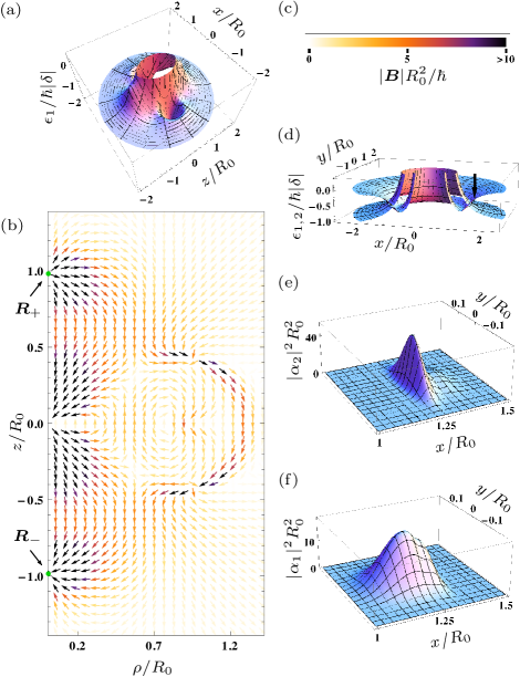
Figure 3: (Color online) (a)-(c) Abelian case. We consider adiabatic motion in state $|\psi_{1}\rangle$. (a) Potential curve $\epsilon_{1}$ in the $x-z$ plane for $\Delta=-3|\delta|$. (b) Artificial magnetic field $\boldsymbol{B}$ in the $\rho-z$ plane. $\boldsymbol{R}_{\pm}$ indicate the positions of the magnetic monopoles. (c) Color code for the absolute value of the effective magnetic field in (b). (d)-(f) Non-Abelian case. We consider non-adiabatic motion in states $|\psi_{1}\rangle$ and $|\psi_{2}\rangle$ for $\Delta=-1.16|\delta|$. (d) Potential curves $\epsilon_{1}$ and $\epsilon_{2}$ in the $x-y$ plane. The initial position of the Gaussian wavepacket in the upper well $\epsilon_{2}$ is indicated by a black arrow. (e) and (f) show the probability density of the evolved wave functions $\alpha_{1}$ and $\alpha_{2}$ at $t|\delta|=220$. The population in the upper (lower) well state $|\psi_{2}\rangle$ ($|\psi_{1}\rangle$) is $52.7\,\%$ ($47.3\,\%$). In (e) and (f), we consider ³⁹K atoms with principal quantum number $n=20$, $|\delta|=2\pi\times 24.7\,\text{MHz}$ and $R_{0}=1.28\mu\text{m}$.

The spatial variation of the vector potential determines the magnetic field $\boldsymbol{B}$ according to Eq. (5). We find that $\boldsymbol{B}$ is only different from zero if $\delta\not=\Delta$ such that the symmetry of the system is broken. In contrast, for a symmetric level scheme the expectation value of $J_{z}$ in Eq. (7) yields zero. Figure 3(b) shows the magnetic field in the $\rho-z$ plane for $\Delta=-3|\delta|$. The most remarkable features of $\boldsymbol{B}$ are a source and a drain of magnetic flux near $\boldsymbol{R}_{+}\approx+0.98R_{0}\boldsymbol{e}_{z}$ and $\boldsymbol{R}_{-}\approx-0.98R_{0}\boldsymbol{e}_{z}$, respectively. We integrate the magnetic field over a sphere $S_{\pm}$ centered at $\boldsymbol{R}_{\pm}$ and evaluate the Chern number xiao:10 $\mathcal{C}_{\pm}=\int_{S_{\pm}}\boldsymbol{B}\cdot\text{d}\boldsymbol{S}/(2\pi)$. The result is $\mathcal{C}_{\pm}=\pm 1$, demonstrating that our system exhibits two magnetic monopoles on the $z$ axis. We emphasize that the monopoles arise at an atomic separation roughly given by $R_{0}$. This parameter can be controlled by the magnitude of the dipole-dipole interaction and the Stark splitting, and is typically of the order of one micron.

Next we show that the artificial magnetic field gives rise to a sizeable deflection of the relative atomic motion. To this end, we suppose that the relative position of the two atoms is initially given by $\boldsymbol{R}_{\text{I}}=R_{0}(-1.5\boldsymbol{e}_{z}+0.05\boldsymbol{e}_{x})$. The initial velocity of the relative motion is $\langle\boldsymbol{v}\rangle=v_{0}\boldsymbol{e}_{z}$ with $v_{0}>0$ such that the atoms move towards the region of strong magnetic fields near $\boldsymbol{R}_{-}$. Here we treat the relative atomic motion classically, which is justified if the wavepacket associated with the relative motion is very well localized. Since $\boldsymbol{R}_{\text{I}}$ contains a small offset in the positive $x$ direction, the potential curve $\epsilon_{1}$ will result in a deflection in the positive $x$ direction [see Fig. 3(a)]. Note that our choice of initial conditions and the azimuthal symmetry of the system imply that the motion remains in the $x-z$ plane if there were no magnetic fields. However, the magnetic field pointing towards $\boldsymbol{R}_{-}$ yields to a deflection $y_{-}$ in the negative $y$ direction via the Lorentz force. On the contrary, the magnetic field will have the opposite effect if we mirror our initial conditions at the $y-z$ plane, i.e., for $\boldsymbol{\tilde{R}}_{\text{I}}=R_{0}(-1.5\boldsymbol{e}_{z}-0.05\boldsymbol{e}_{x})$. In this case, the relative motion remains in the $x<0$ half plane and the Lorentz force results in a deflection $y_{+}$ in the positive $y$ direction. It follows that the difference $\Delta y=y_{+}-y_{-}$ is a direct measure of the effective magnetic field. In addition, it reflects the broken chiral symmetry arising from the asymmetric level scheme in Fig. 1(b).

In order to obtain a quantitative description of this effect, we derive a set of coupled equations for the mean values $\langle\boldsymbol{R}\rangle$ and $\langle\boldsymbol{v}\rangle$ from the Hamiltonian $H$ in Eq. (1) tannoudji:lc . We consider ²³Na atoms with principal quantum number $n=15$ and $|\delta|=2\pi\times 39.0\,\text{MHz}$ comment1 . This yields $R_{0}=0.75\mu\text{m}$, and hence the distance between the atoms is initially given by $|\boldsymbol{R}_{\text{I}}|=|\boldsymbol{\tilde{R}}_{\text{I}}|\approx 1.13\mu\text{m}$. Furthermore, we set $v_{0}=195\hbar/(R_{0}\mu)$. We neglect effects due to the finite lifetime of the molecule ($T|\delta|\approx 540$) and thus restrict the analysis to times $t\leq T$. From semi-classical simulations for the two initial positions $\boldsymbol{R}_{\text{I}}$ and $\boldsymbol{\tilde{R}}_{\text{I}}$ we find $\Delta y=0.1R_{0}$ for $t|\delta|=238$, and $\Delta y=0.3R_{0}$ at $t|\delta|=483$. It follows that the magnetic field results in a substantial deflection of the relative atomic motion. Note that our simulations allow us to confirm that the motion remains adiabatic at all times.

Next we show that the vector potential $\boldsymbol{A}$ can give rise to a coupling between the relative atomic motion and internal electronic states. In order to demonstrate this synthetic spin-orbit coupling, we consider an additional potential curve $\epsilon_{2}$ with corresponding state $|\psi_{2}\rangle$. Here we focus on the two-dimensional setting where the motion is confined to the $x-y$ plane. The two potential curves $\epsilon_{1}$ and $\epsilon_{2}$ become near-degenerate for $R\approx 1.33R_{0}$ and $\Delta=-1.16|\delta|$ and are shown in Fig. 4(a). In order to investigate the quantum dynamics in the two cylindrically symmetric potential wells, we evaluate the vector potential $\boldsymbol{A}$ in Eq. (4) by numerical means jpb . Note that $\boldsymbol{A}$ is now represented by a $2\times 2$ matrix, where each component $\boldsymbol{A}_{kl}$ is a 3-column vector. We find that the component $A^{(3)}$ is zero, and the non-zero parts of $A^{(1)}$ and $A^{(2)}$ are shown in Figs. 4(b) and (c), respectively. All components of $\boldsymbol{A}$ are evaluated for $\phi=0$ such that $A^{(1)}$ ($A^{(2)}$) can be identified with the radial (azimuthal) component of $\boldsymbol{A}$.

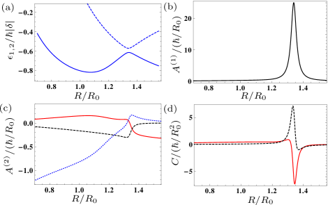
Figure 4: (Color online) (a) Potential curves $\epsilon_{1}$ (solid blue line) and $\epsilon_{2}$ (dashed blue line) in the $x-y$ plane. (b) Imaginary part of $A_{12}^{(1)}=[A_{21}^{(1)}]^{*}$ for $\phi=0$. (c) Real parts of $A_{11}^{(2)}$ (solid red line), $A_{22}^{(2)}$ (dashed black line) and $A_{12}^{(2)}=[A_{21}^{(2)}]^{*}$ (dotted blue line) for $\phi=0$. (d) Matrix elements of the commutator $C=\imath[A^{(1)},A^{(2)}]/\hbar$. The red solid line shows $C_{11}=-C_{22}$, and the black dashed line represents $C_{12}=C_{21}$. In (a)-(d), we set $\Delta=-1.16|\delta|$. All components of $\boldsymbol{A}$ that are not shown in (b) and (c) are zero.

Near the avoided crossing the off-diagonal element $\boldsymbol{A}_{12}$ can induce non-adiabatic transitions between the states $|\psi_{1}\rangle$ and $|\psi_{2}\rangle$. The coupling strength depends on the energy difference $|\epsilon_{1}-\epsilon_{2}|$ and the velocity of the relative motion. For a quantitative description of this synthetic spin-orbit coupling, we assume that the system is initially at rest and prepared in the upper well state $|\psi_{2}\rangle$ [see Fig. 3(d)]. We model the wavepacket corresponding to the relative atomic motion by a Gaussian with a full width at half maximum of $\sigma\approx 75\,\text{nm}$ centered at $R=1.5R_{0}$ and solve Eq. (3) for $q=2$ in a box with radius $2.2R_{0}$. As the system evolves, it will oscillate in the upper well, and near the avoided crossing some population will be coherently transferred to the lower well state $|\psi_{1}\rangle$. The probability densities in the two states after the avoided crossing has been traversed once is shown in Figs. 3(e) and (f). For the chosen parameters an almost equal superposition of the two internal states is created. Note that the two wavepackets experience different potentials [see Fig. 4(a)] and hence they will separate in space for longer evolution times.

We emphasize that the gauge fields $A^{(1)}$ and $A^{(2)}$ are strongly non-Abelian as shown in Fig. 4(d). The commutator $C=\imath[A^{(1)},A^{(2)}]/\hbar$ is of the same order of magnitude as the first term in Eq. (6), and thus the non-Abelian signature is significant whenever the magnetic field gives rise to sizeable effects in the quantum dynamics of the system. This opens up the possibility to study the rich physics resulting from non-Abelian gauge fields jacob:07 , which is subject to further investigation.

In summary, we have shown that the dipole-dipole interaction between Rydberg atoms can induce Abelian and non-Abelian artificial gauge fields that influence the relative atomic motion significantly. The experimental realization of our scheme could be achieved in optical lattices where the lattice constant matches the desired initial separation of the atoms. Alternatively, one could start with a similar setup as described in gaetan:09 ; urban:09 , where the dipole-dipole interaction between two individual Rydberg atoms trapped in optical tweezers was investigated. The optical potentials allow one to control the initial position of the atoms before they are excited to the diatomic $nsns$ state via laser fields. A subsequent microwave field prepares the system in the desired $nsnp$ state $|\psi_{1}\rangle$ or $|\psi_{2}\rangle$. In addition, the optical trapping potentials could transfer linear momentum to the atoms before the excitation to the Rydberg states occurs. Our calculations for the deflection in the monopole field were carried out at zero temperature. By considering a thermal velocity distribution, we estimate that the deflection pattern will be washed out if the temperature exceeds approximately $100\,\text{nK}$. These temperatures are routinely achieved in optical lattices and dipole traps arnold:11 . Finally, the observation of the relative atomic motion requires measurements of the density-density correlations of the two Rydberg atoms. Such measurements have been performed by ionization of the Rydberg atoms schwarzkopf:11 and by de-excitation to the ground state followed by advanced imaging techniques schauss:12 . We thus believe that the experimental observation of the deflection in the monopole field and the splitting of the motional wavepacket is feasible with current or next-generation imaging techniques.

References

- (1) J. Ruseckas, G. Juzeliūnas, P. Öhberg, and M. Fleischhauer, Phys. Rev. Lett. 95, 010404 (2005)
- (2) J. Dalibard, F. Gerbier, G. Juzeliūnas, and P. Öhberg, Rev. Mod. Phys. 83, 1523 (2011)
- (3) R. Dum and M. Olshanii, Phys. Rev. Lett. 76, 1788 (1996)
- (4) Y.-J. Lin, R. L. Compton, A. R. Perry, W. D. Phillips, J. V. Porto, and I. B. Spielman, Phys. Rev. Lett. 102, 130401 (2009)
- (5) Y.-J. Lin, R. L. Compton, K. Jiménez-García, J. V. Porto, and I. B. Spielman, Nature 462, 628 (2009)
- (6) Y.-J. Lin, R. L. Comption, K. Jiménez-García, W. D. Phillips, J. V. Porto, and I. B. Spielman, Nat. Phys. 7, 531 (2011)
- (7) M. Aidelsburger, M. Atala, S. Nascimbène, S. Trotzky, Y.-A. Chen, and I. Bloch, Phys. Rev. Lett. 107, 255301 (2011)
- (8) D. Jaksch and P. Zoller, New. J. Phys. 5, 56 (2003)
- (9) J. Struck, C. Ölschläger, R. L. Targat, P. Soltan-Panahi, A. Eckardt, M. Lewenstein, P. Windpassinger, and K. Sengstock, Science 333, 996 (2011)
- (10) J. Struck, C. Ölschläger, M. Weinberg, P. Hauke, J. Simonet, A. Eckardt, M. Lewenstein, K. Sengstock, and P. Windpassinger, Phys. Rev. Lett. 108, 225304 (2012)
- (11) K. Jiménez-García, L. J. LeBlanc, R. A. Williams, M. C. Beeler, A. R. Perry, and I. B. Spielman, Phys. Rev. Lett. 108, 225303 (2012)
- (12) P. Hauke, O. Tieleman, A. Celi, C. Ölschläger, J. Simonet, J. Struck, M. Weinberg, P. Windpassinger, K. Sengstock, M. Lewenstein, and A. Eckardt, Phys. Rev. Lett. 109, 145301 (2012)
- (13) J. Moody, A. Shapere, and F. Wilczek, Phys. Rev. Lett. 56, 893 (1986)
- (14) M. Born and J. R. Oppenheimer, Annalen der Physik 389, 457 (1927)
- (15) C. Boisseau, I. Simbotin, and R. Cotè, Phys. Rev. Lett. 88, 133004 (2002)
- (16) N. Samboy, J. Stanojevic, and R. Cote, Phys. Rev. A 83, 050501(R) (2011)
- (17) M. Kiffner, H. Park, W. Li, and T. F. Gallagher, Phys. Rev. A 86, 031401(R) (2012)
- (18) K. R. Overstreet, A. Schwettmann, J. Tallant, D. Booth, and J. P. Shaffer, Nat. Phys. 5, 581 (2009)
- (19) A. Schwarzkopf, R. E. Sapiro, and G. Raithel, Phys. Rev. Lett. 107, 103001 (2011)
- (20) P. Schauß, M. Cheneau, M. Endres, T. Fukuhara, S. Hild, A. Omran, T. Pohl, C. Gross, S. Kuhr, and I. Bloch, Nature 491, 87 (2012)
- (21) A. Gaëtan, Y. Miroshnychenko, T. W. an A. Chotia, M. Viteau, D. Comparat, P. Pillet, A. Browaeys, and P. Grangier, Nat. Phys. 5, 115 (2009)
- (22) E. Urban, T. A. Johnson, T. Henage, L. Isenhower, D. D. Yavuz, T. G. Walker, and M. Saffman, Nat. Phys. 5, 110 (2009)
- (23) F. Wilczek and A. Zee, Phys. Rev. Lett. 52, 2111 (1984)
- (24) M. Kiffner, W. Li, and D. Jaksch, in preparation.
- (25) D. Xiao, M.-C. Chang, and Q. Niu, Rev. Mod. Phys. 82, 1959 (2010)
- (26) See, e.g., complement AV in: C. Cohen-Tannoudji, J. Dupont-Roc, and G. Grynberg, Atom- Photon Interactions (Wiley, New York, 1998).
- (27) The moment of inertia increases with principal quantum number . For our setup we find that values of maximize the mechanical effects of the artificial gauge fields on the relative atomic motion.
- (28) A. Jacob, P. Öhberg, G. Juzeliūnas, and L. Santos, Appl. Phys. B 89, 439 (2007)
- (29) K. J. Arnold, and M. D. Barrett, Optics Comm. 284, 3288-3291 (2011).