Stable and Informative Spectral Signatures for Graph Matching

Abstract

In this paper, we consider the approximate weighted graph matching problem and introduce stable and informative first and second order compatibility terms suitable for inclusion into the popular integer quadratic program formulation. Our approach relies on a rigorous analysis of stability of spectral signatures based on the graph Laplacian. In the case of the first order term, we derive an objective function that measures both the stability and informativeness of a given spectral signature. By optimizing this objective, we design new spectral node signatures tuned to a specific graph to be matched. We also introduce the pairwise heat kernel distance as a stable second order compatibility term; we justify its plausibility by showing that in a certain limiting case it converges to the classical adjacency matrix-based second order compatibility function. We have tested our approach on a set of synthetic graphs, the widely-used CMU house sequence, and a set of real images. These experiments show the superior performance of our first and second order compatibility terms as compared with the commonly used ones.

1 Introduction

Graph matching techniques have been widely used in computer vision in contexts such as 2D and 3D image analysis, object recognition, biomedical identification, and object tracking. Most practical problems require using approximate matching algorithms that can extract meaningful correspondences even when the graphs under consideration are not isomorphic. Therefore, when using the common quadratic assignment formulation of graph matching problem, it is desirable to have informative first and second order compatibility terms that are stable to violations of isomorphism.

Spectral approaches [31, 6, 9, 12, 33, 8] have been widely used in graph matching literature. Recently, spectral node signatures (first order compatibility terms) such as the heat kernel signature (HKS) [30] and the wave kernel signature (WKS) [2] have been drawing significant attention for matching of 3D shapes in computer graphics. These constructions are inspired by physical processes (e.g. heat propagation) on graphs, and are expected to inherit the physical processes’ stability to perturbations of the underlying graph. However, the analysis of stability of spectral signatures in general is lacking, which hinders the ability to design spectral node signatures that are not derived from physical processes. While there has been some work on learning such signatures for 3D shapes [21, 1], they require a training set of one form or another, which may be difficult to obtain.

The goal of our work is to establish general theoretical results about the stability of first and second order terms constructed from graph Laplacians [14], and to use these results in a practical graph matching framework; we are especially interested in designing node signatures tuned to the graphs being matched. We start out with a family of spectral node signatures, which we call the Laplacian Family Signatures (LFS). This family is parametrized by a real-valued function of two variables – the construction filter; particular choices of the construction filter yield the HKS and WKS as special cases. We first establish a stability result for the LFS, obtaining an upper bound on how much the signature of a node can change under perturbations of the underlying graph. Next, we relax the bounds in our stability theorem, which allows us to encode both the requirements of stability and informativeness in a single objective function. By optimizing this objective, we obtain a custom construction filter and so a custom spectral node signature for matching the graph under consideration.

While the steps above yield a stable first order compatibility term, stability of the second order compatibility term is as important. Another contribution of this work is to introduce the pairwise heat kernel distance as a second order compatibility term suitable for inclusion into the Integer Quadratic Program (IQP) formulation of the graph matching problem. This term can be shown to be stable to perturbations of the underlying graph. To justify its use as a second order term we prove that in a certain limiting case, the pairwise heat kernel distance reproduces the commonly used term obtained from the adjacency matrices.

Our overall practical graph matching approach has a number of benefits. First, our approach is based on rigorous theoretical results on stability of node and edge signatures, that are of independent interest. Second, despite the fact that our construction filter is non-parametric, we obtain a simple convex optimization problem that can be solved efficiently. Third, in contrast to previous methods, e.g. [1], we do not require a training set, but base our node signature optimization on the given graph to be matched. Ideally, signature design should be based on a representative “average” graph of the collection of graphs arising in a specific context. However, computing the average graph itself requires reliable matchings between all graphs in the collection, leading to a chicken-and-egg problem. To circumvent this, we hypothesize that an attempt to match a given graph to other graphs in a collection – if it is to be at all successful – is indicative of shared structure, and this should allow optimizing signatures based solely on the graph that is being matched. Our experimental results confirm that signatures optimized in such a way provide superior results over un-optimized signatures in a number of settings.

The rest of the paper is organized as follows. After reviewing previous work in Section 2, we introduce and analyze the first order compatibility terms in Section 3. The second order compatibility term is introduced in Section 4. The IQP for quadratic assignment formulation of graph matching problem is set up in Section 5. We present our experimental results on three different graph matching tasks in Section 6.

2 Related Work

Node-based signatures have been popular in the context of graph matching. Joilli et. al.[16] proposed a signature composed of the degree of the a node followed by the ordered weights of each incident edge and padded with zero if necessary. Gori et. al. [12] constructed node signatures from the steady state distributions of simulated random walks similar to PageRank. Eshera [10] built signatures for attributed relational graphs (ARG). Shokoufandeh et. al [28] constructed feature-based node signatures for bipartite matching. The same authors [29] later proposed a topological signature vector (TSV) for directed acyclic graphs (DAG). Hu et. al [15] considered graph matching from the learning of a signature-based proximity matrix using disclosed known correspondences without explicitly computing the signatures themselves.

Node signatures used in our work are most closely related to spectral methods for graph matching. Among the pioneering works is Umeyama’s [31] weighted graph matching algorithm , which was later generalized to graphs of different sizes [22, 37]. Robles-Kelly et. al. [25] ordered the nodes from the steady state of Markov chain with the edge connectivity constraint and matched using edit distance; in [26], they ordered the nodes using the leading eigenvector of the adjacency matrix. Qiu et. al [24] considered using Fiedler vector to partition the graph for hierarchical matching; their method, however, works only on planar graphs. Cho et. al. [5] constructed reweighted random walks similar to personalized PageRank on the association graph with the addition of an absorbing node. They computed its quasi-stationary distribution and discretized the continuous solution to find a matching. Emms et. al. [9] built an auxiliary graph from the two graphs and simulated a quantum walk. Particle probability of each auxiliary node was used as the cost of assignment for a bipartite matching.

In a broader sense of relatedness to our work are other relaxation-based matching algorithms. Gold and Rangarajan [11] proposed the well-know Graduated Assignment Algorithm. van Wyk et. al. [32] designed a projection onto convex set (POCS) based algorithm to solve IQP by successively projecting the relaxed solution onto the convex constraint set. Schellewald et. al. [27] constructed a semidefinite programming relaxation of the IQP. Leordeanu et. al. [19] proposed a spectral method to solve a relaxed IQP where they drop the linear inequality constraint during relaxation and only incorporate it at the discretization step. The idea was further extended by Cour et. al. [6], where they added an affine constraint during relaxation. Zaslavskiy et. al. [35] approached the IQP from the point of a relaxation of the original least-square problem to a convex and concave optimization problem on the set of doubly stochastic matrices. Leordeanu et. al. [20] proposed an integer projected fixed point (IPFP) algorithm to solve the quadratic assignment problem. Zhou et. al. [38] proposed a factorized graph matching algorithm to solve IQP problem by factorizing the affinity matrix into the Kronecker product of smaller matrices.

3 First Order Compatibility

In this section, we introduce the Laplacian Family Signatures (LFS) as a structural descriptor for graph nodes. We then establish a stability theorem showing the robustness of these descriptors to perturbations of the graph. Next, for a given graph, we will show how the bounds established by our stability theorem together with considerations of informativeness can be used to choose an optimal signature from this family of signatures.

3.1 Laplacian Family Signatures

Consider one of the graphs to be matched, say $G=(V,E)$. Let $w$ be the weights on edges, i.e. $w:E\mapsto\mathbb{R}^{+}$. The graph Laplacian is defined as ${\cal L}=D-A$, where $A$ is the graph adjacency matrix, and $D$ is a diagonal matrix of total incident weights, i.e. $D_{ii}=\sum_{j}{A_{ij}}$. ${\cal L}$ has numerous useful properties [3], of which most relevant to us is its symmetry and positive semi-definiteness. This makes it possible to consider the eigen-decomposition of ${\cal L}$; we denote by $\{\lambda_{k},\phi_{k}\}_{k=1}^{|V|}$ the eigenpairs (eigenvalue and associated eigenvector) of the graph Laplacian matrix ${\cal L}$.

The eigenvalues and eigenvectors of the Laplacian matrix carry a wealth of structural information about the underlying weighted graph. Our goal is to use this information to obtain signatures for nodes of the graph that are both stable and informative. We first start with a very general definition of a family of signatures.

Definition 1

For a given real valued function $h(\cdot;\cdot):\mathbb{R}_{+}^{2}\rightarrow\mathbb{R}$, the Laplacian Family Signature (LFS) of a node $i\in V$ is a one-parameter family of structural node descriptors that is defined by

$$s_{i}(t)=\sum_{k}h(t;\lambda_{k})\phi_{k}(i)^{2}.$$ (1)

We refer to $h(\cdot;\cdot)$ as the construction filter.

The Laplacian Family Signatures describe a given node’s structural relationship to its neighborhood at large (see e.g. physical interpretation of signatures in the next subsection). Note that the signature of a given node $i\in V$ is itself a function $s_{i}(\cdot):\mathbb{R}_{+}\rightarrow\mathbb{R}$. Thus, two nodes $i$ and $a$ from the same or different graphs can be compared by using any kind of distance/norm between the functions $s_{i}(\cdot)$ and $s_{a}(\cdot)$.

A number of particular choices of the construction filter have been considered in previous work. Choosing $h(t;\lambda_{k})=\exp(-t\lambda_{k})$ results in the heat kernel signature (HKS) [30], and selecting $h(t;\lambda_{k})=\exp(-\frac{(t-\log\lambda_{k})^{2}}{2\sigma^{2}})$, one obtains the wave kernel signature (WKS) [2]; these signatures were shown to have desirable properties for applications in 3D shape analysis and matching. Assuming that $h(t;\lambda_{k})=g(t\lambda_{k})$ is a band-pass filter with a special behavior as in [13], we can easily obtain another signature – the wavelet kernel signature.

It is clear that a plethora of such descriptors can be obtained by simply varying the construction filter. An important question is then what choice of the filter is optimal in one or another sense. We address this issue in the following two subsections by considering two conflicting requirements – the informativeness and stability of signatures.

3.2 General Stability Result

The LFS signatures are naturally intrinsic: if two graphs are isomorphic, then the signatures of corresponding nodes are the same. However, for a signature to be practically useful, it should also be stable under perturbations of the graph. Stability of existing signatures, such as HKS and WKS, are derived from intuitive considerations based on physical interpretations. For example, HKS has an interpretation in terms of a simulated heat diffusion process [30]: for each node, this signature captures the amount of heat left at the node at various times (here $t$) assuming that a unit amount is put on the node initially ($t=0$). WKS also has a physical interpretation in terms of a quantum mechanical process on the graph [2]. The stability then follows from the assumption that these physical processes are stable under small perturbations of the underlying graph.

One of our main results is to establish the stability of LFS signatures in general without a recourse to a physical interpretation. Importantly, we obtain upper bounds on how much the signatures may change, and we consider both the case of distinct and repeating eigenvalues.

Theorem 1

Let $A,A^{\prime}$ be the adjacency matrices of a pair of graphs, and ${\cal L},{\cal L}^{\prime}$ be the induced Laplacians. Let the size of the graph be $n$, and $\lambda_{1}<\cdots<\lambda_{k}$ denote the $k$ distinct eigenvalues of ${\cal L}$. Let $s_{i}(t)$ and $s^{\prime}_{i}(t)$ denote the LFS’s of node $i$. Assume $\lambda_{j+1}-\lambda_{j}\geq\delta,\forall j$, $\|A-A^{\prime}\|_{F}\leq\frac{\epsilon}{\sqrt{n+1}}<\delta$, and $h(\cdot;\cdot)\in C^{2}(\mathbb{R}_{+}^{2})$. If $k=n$ (non-repeating eigenvalues), we have

$$|s^{\prime}_{i}(t)-s_{i}(t)|\leq C_{0}(\delta,t)\epsilon,$$

where $C_{0}(\delta,t)$ is a constant independent of $\epsilon$. If $k<n$ (repeating eigenvalues), we have

$$|s_{i}(t)-s^{\prime}_{i}(t)|\leq C_{1}(t)\left(\frac{\delta}{\delta-\epsilon}-1\right)+C_{2}(t)\epsilon,$$

where $C_{1}(t),C_{2}(t)$ are constants depending only on $t$.

See supplementary material for a proof. Even a more general stability result when the number of graph nodes changes can be obtained using lifting ideas similar to [29].

3.3 Signature Optimization

In addition to stability, a practically useful signature has to be informative. For a special category of compact Riemannian manifolds, both HKS and WKS have been shown to be informative, e.g. Theorem 1 in [30], i.e. they fully characterize the shapes up to isometry. For general graphs, however, the informativeness could hardly be well-defined, as one could easily find counter examples such that non-isomorphic graphs share the same LFS. In the context of graph matching, nonetheless, we could still intuitively explain informativeness of LFS as structural richness. This is why instead of a single number, the LFS describes a node $i\in V$ by a function $s_{i}(\cdot):\mathbb{R}_{+}\rightarrow\mathbb{R}$. However, this does not directly guarantee the informativeness of the signature, because the function values $s_{i}(t)$ may be strongly correlated with each other at different values of $t$, reducing the information content of the descriptor.

Interestingly, the requirements of informativeness and stability are conflicting. Indeed, our stability theorem shows that the signatures are more stable when the construction filter is smooth. On the other hand, the information content is maximized when the construction filter concentrates as much as possible (like a delta function) at a given eigenvalue, thereby extracting information from non-overlapping frequency bands of eigenvectors.

Both of these conflicting requirements can be captured by relaxing the bounds established in Theorem 1. As can be seen (c.f. supplementary material) in both distinct ($k=n$) and repeated ($k<n$) eigenvalue cases, the upper bound depends on two terms – $\max_{j}|h(t,\lambda_{j})|$ and $\max_{j}|\frac{\partial}{\partial\lambda}h(t,\lambda_{j})|$. Taking the $L^{1}$-norm as the distance metric when comparing signatures, we can bound the change in signature of a node $i\in V$ under perturbation (c.f. Theorem 1) as

$$d(s_{i},s^{\prime}_{i}) = \int|s_{i}(t)-s^{\prime}_{i}(t)|\textnormal{d}t$$ (2)

$$\leq \frac{2\epsilon}{\delta}\left(\int\max_{j}\left|h(t;\lambda_{j})\right|\textnormal{d}t\right)$$

$$+\epsilon\left(\int\max_{j}\left|\frac{\partial}{\partial\lambda}h(t;\lambda_{j})\right|\textnormal{d}t\right)$$

To minimize this upper bound, we, nevertheless, have two contradicting terms unless we use the trivial solution $h\equiv 0$ everywhere. The first term requires $h(t;\lambda)$ concentrate on $\lambda$, i.e. it should be as narrow as possible on each distinct frequency $\lambda_{j}$ (informativeness). The second term, on the other hand, requires $h(t;\lambda)$ to be smooth at $\lambda$, i.e. it should be as wide as possible at each distinct frequency $\lambda_{j}$ (stability).

When a meaningful matching between two graphs exists, it is natural to assume that one of the graphs is a perturbation of the other. Based on this intuition, we propose to pick one of the graphs as the source graph, and to determine an optimal (with respect to the upper bound above) construction filter $h(t;\lambda)$ for the source graph. Then the graphs are matched using this optimal filter on both the source and target graphs.

To find the optimal construction filter $h(\cdot;\cdot)$ for a given source graph, we will minimize the upper bound above. To simplify our optimization problem, note that for informativeness, we need $h(t;\lambda)$ to be large at $\lambda$ while fading away farther from $\lambda$, and so we assume $h(t;\lambda)$ to be of the form $h(|t-\lambda|)$ with $h(0)=1$. We will also restrict $h$ to be positive and uniformly decreasing. Finally, the requirement of $h(\cdot)\in C^{2}(\mathbb{R}_{+}^{2})$ is achieved by putting a bound on the second derivative $h^{\prime\prime}(\cdot)$.

The simplified optimization problem becomes that of finding $h:\mathbb{R}_{+}\rightarrow\mathbb{R}$ solving

$$\begin{array}[]{ll}\min&\mu\int\max_{j}h(|t-\lambda_{j}|)\textnormal{d}t+\int\max_{j}|h^{\prime}(|t-\lambda_{j}|)|\textnormal{d}t\\ \textnormal{s.t.}&h(0)=1,\>h(x)\geq 0,\>h^{\prime}(x)\leq 0,\>|h^{\prime\prime}(x)|\leq c_{h}\end{array}$$

where the parameter $\mu=\frac{2}{\delta}$ is expressed in terms of the eigen-gap $\delta$. In practice, we set $\delta$ to be the average eigen-gap of the eigenvalue sequence. As it is clear from the objective function, in addition to the eigen-gap, the optimal filter will depend on the entire eigenvalue distribution of the Laplacian.

While the above problems may be hard to solve analytically, it can be straightforwardly discretized and solved numerically as a convex optimization problem. In practice, w.l.o.g., we consider $h(|t|)$ to be non-zero only on $[-T,T]$. Symmetric as it is, we only need to evenly sample $h$ on $[0,T]$ as a vector $\mathbf{h}=\left[h_{0},\cdots,h_{N}\right]^{\top}$, with $h_{0}=1,h_{N}=0$. Let $\Delta h$ be the step between samples. The first and second order derivative could be numerically estimated as $\mathbf{h}^{\prime}=\left[\frac{h_{1}-h_{0}}{\Delta h},\cdots,\frac{h_{N}-h_{N-1}}{\Delta h}\right]^{\top}$ and $\mathbf{h}^{\prime\prime}=\left[\frac{h_{2}-h_{0}}{\Delta h^{2}},\cdots,\frac{h_{N}-h_{N-2}}{\Delta h^{2}}\right]^{\top}$. Let $\mathbf{h}_{j}$, $\mathbf{h}^{\prime}_{j}$, $\mathbf{h}^{\prime\prime}_{j}$ be the $\lambda_{j}$-shifted version of $\mathbf{h}$, $\mathbf{h}^{\prime}$, $\mathbf{h}^{\prime\prime}$ (padded with zeros if needed). The discretized optimization problem could therefore be written as

$$\min{} ~{}\mu\mathbf{1}^{\top}\max(\mathbf{h}_{1},\cdots,\mathbf{h}_{k})+\mathbf{1}^{\top}\max(\mathbf{h}^{\prime}_{1},\cdots,\mathbf{h}^{\prime}_{k})$$

s.t. $$~{}\mathbf{h}_{i}\geq 0,~{}\mathbf{h}^{\prime}_{i}\leq 0,~{}-c_{h}\leq\mathbf{h}^{\prime\prime}_{i}\leq 0,~{}h_{0}=1,~{}h_{N}=0$$

where $\mathbf{1}$ is the unit vector and $\max(\cdot)$ is the element-wise max among its arguments.

Figure 1(a) shows the optimal filters for several types of randomly generated graphs . The LFS with our optimized kernel is named ”adaLFS” (for adaptive LFS) in all the figures that follow. The improved matching results on some well-known dataset can be seen in Figures 1(b), 1(c), and will be more thoroughly discussed in Section 6.

4 Stable Second Order Compatibility

In this section, we introduce a second order compatibility term based on the heat diffusion process on graphs. Specifically, consider the graph heat kernel $k_{t}(i,j)$, which measures the amount of heat transferred from node $i$ to node $j$ after time $t$, assuming a unit amount was placed at $i$ in the beginning ($t=0$). The heat kernel has the following representation in terms of the eigen-decomposition of the graph Laplacian:

$$k_{t}(i,j)=\sum_{k}\exp(-t\lambda_{k})\phi_{k}(i)\phi_{k}(j).$$

Using an argument similar to the proof of Theorem 1, one can establish stability of $k_{t}(\cdot,\cdot)$ to perturbations (see supplementary material). Therefore, it provides a natural choice for a second order compatibility term.

Definition 2

Let $k_{t}$ and $k^{\prime}_{t}$ be the heat kernels of $G=(V,E)$ and $G^{\prime}=(V^{\prime},E^{\prime})$ respectively. For $i,j\in V$ and $a,b\in V^{\prime}$, the pairwise heat kernel distance is defined as

$$d_{t}^{{\cal K}}(i,j,a,b)=\left|k_{t}(i,j)-k^{\prime}_{t}(a,b)\right|.$$

We will compare this term with the commonly used term based on the adjacency matrices $A,A^{\prime}$ of the graphs $G,G^{\prime}$:

$$d^{A}(i,j,a,b)=\left|A_{ij}-A^{\prime}_{ab}\right|.$$

The following theorem shows that the pairwise heat kernel distance $d_{t}^{{\cal K}}$ is a stable approximation of the pairwise adjacency distance $d^{A}$ (see supplementary material for a proof).

Theorem 2

Let $d_{t}^{{\cal K}}(i,j,a,b)$ and $d^{A}(i,j,a,b)$ be the pairwise heat kernel distance and pairwise adjacency distance for graph $G$ and $G^{\prime}$, then the following holds:

$$\lim_{t\rightarrow 0}\frac{d_{t}^{{\cal K}}(i,j,a,b)}{t}=d^{A}(i,j,a,b).$$

When $t$ is small, $d_{t}^{{\cal K}}$ is a good approximation of $d^{A}$; as $t$ increases, $d_{t}^{{\cal K}}$ is smoothed out. In this way it becomes stable, because in the ideal case when the graphs are isomorphic, $d^{A}$ should be zero everywhere for matched pairs.

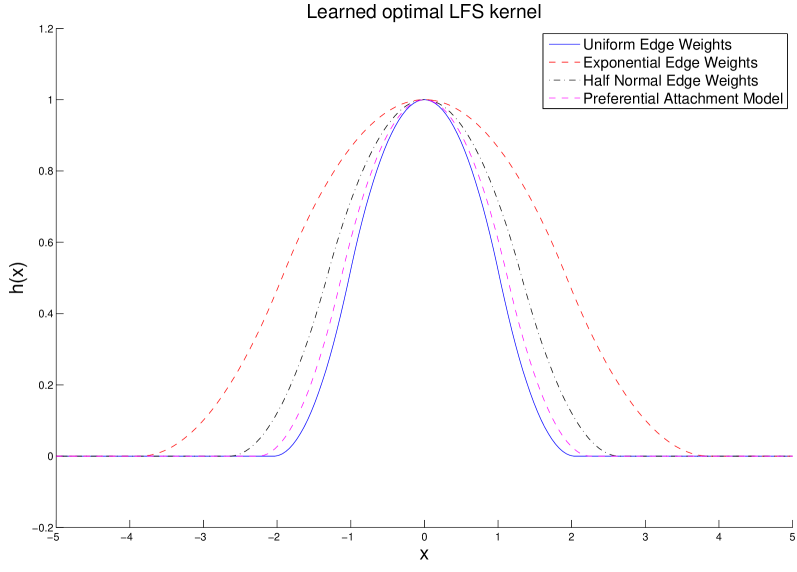
(a)

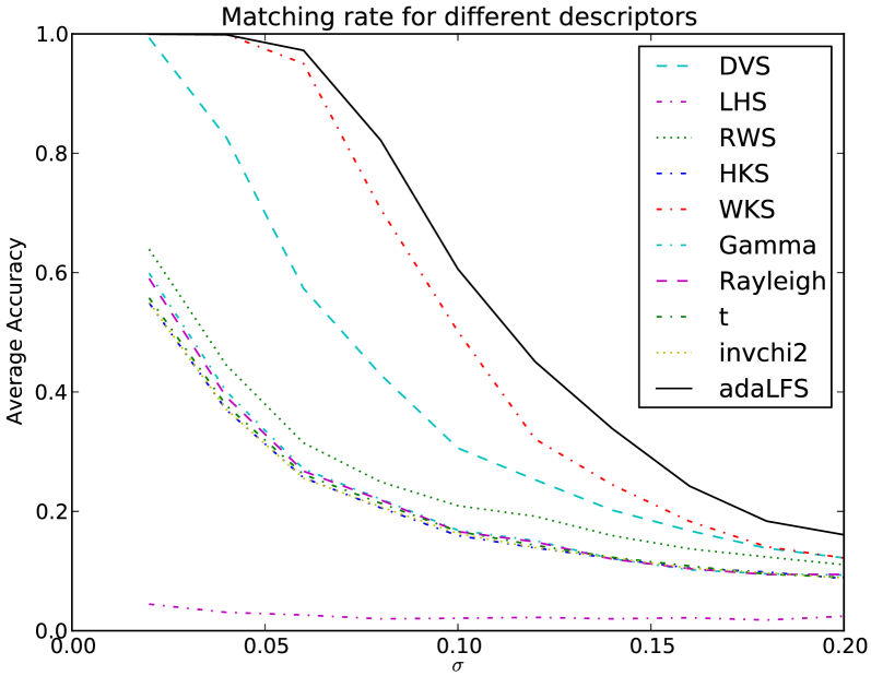
(b)

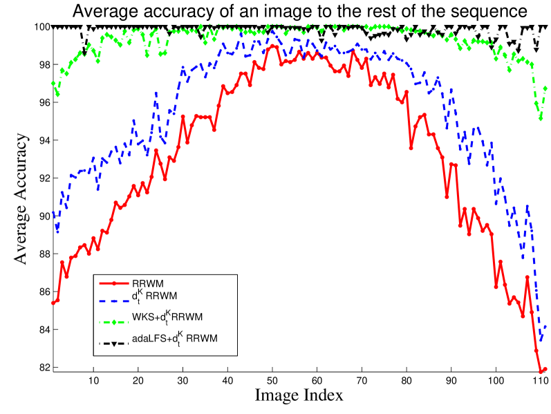
(c)

Figure 1: (a) Optimal construction filters for different types of random graphs (red) and an image key points graph (blue). (b) Signature comparison for $G(n,m)$ random graphs. (c) Matching accuracy for CMU House sequence.

5 Matching Scheme

To directly compare the performance within LFS and with other node signatures, the problem is cast as a bipartite graph matching problem as in existing node signature based matching work [28, 12, 16], where costs are set as the distances between signatures. The problem is solved using Hungarian algorithm [17].

For practical matching, in addition to node signatures, we use the pairwise heat kernel distance $d_{t}^{{\cal K}}$ as the second order constraint and formulate the problem as an integer quadratic program (IQP). Namely, for two graphs $G=(V,E)$ and $G^{\prime}=(V^{\prime},E^{\prime})$ to be matched and nodes $i\in V,a\in V^{\prime}$, let $d(i,a)$ be the distance between their node signatures. We construct the compatibility matrix $W\in\mathbb{R}^{|V||V^{\prime}|\times|V||V^{\prime}|}$ as

$$W_{ia,jb}=\begin{cases}d_{t}^{{\cal K}}(i,j,a,b)&i\neq j,~{}a\neq b\\ \alpha d(i,a)&i=j,~{}a=b\end{cases}$$

Letting $\mathbf{X}\in\{0,1\}^{|V|\times|V^{\prime}|}$ be the one-to-one mapping matrix, and $\mathbf{x}\in\{0,1\}^{|V||V^{\prime}|}$ its vectorization, the IQP can be written as

$$~{}\mathbf{x}^{*}=\arg\min(\mathbf{x}^{\top}W\mathbf{x})$$

s.t. $$~{}\mathbf{x}\in\{0,1\}^{|V||V^{\prime}|},~{}\forall i~{}\sum_{a\in V^{\prime}}\mathbf{x}_{ia}\leq 1,~{}\forall a~{}\sum_{i\in V}\mathbf{x}_{ia}\leq 1$$

As is well-known, this problem is NP-complete and there is a large literature of approximation algorithms. In our experiments, we selected a recently proposed algorithm, the reweighed random walk matching (RRWM) [5] because of its superior performance compared with other state-of-the-art approximation algorithms, including SM [19], SMAC [6], HGM [36], IPFP [20], GAGM [11], SPGM[32]. While finding a good solver for IQP is an interesting problem per se, we will not explore possibilities in this direction as it will inevitably shift the focus of our paper.

6 Experiments

We tested our descriptor on three different datasets: 1) synthetically generated random graphs; 2) CMU House sequence for point matching; 3) feature matching using real images.

6.1 Synthetic Random Graphs

In this section, following the experimental protocol of [5], we synthetically generate random graphs and perform a comparative study. In the first part of the experiment, we use random graphs from Erdös-Rényi model $\textnormal{G}(n,m)$, where $m$ edges are randomly selected from all possible $\frac{n(n-1)}{2}$ edges. For each selected edge, we add a uniform random weight in the range $[0,1]$. The graph is then perturbed by adding random Gaussian noise ${\cal N}(0,\sigma^{2})$ on selected edges.

In this test, we compare the performance within our LFS and with existing node signatures, namely degree vector signature (DVS) [16], local histogram signature (LHS) [34], random walk signature (RWS) [12]. For comparisons within LFS family, we do not limit ourselves to HKS and WKS, which are known special cases of LFS. Noticing that both HKS and WKS construction filters are continuous probability density functions (pdf) of some distribution, we include a number of other pdfs: i) Gamma distribution $(t\lambda_{i})^{k-1}\exp\left(-t\lambda_{i}/\theta\right)$, ii) Gaussian distribution $\exp\left(-(t-\mu(\lambda_{i}))^{2}/2\sigma^{2}\right)$, iii) t-distribution $\left(1+(t\lambda_{i})^{2}/\theta\right)^{-(k+1)/2}$, iv) Rayleigh distribution $(t\lambda_{i})^{k-1}\exp\left(-(t\lambda_{i})^{2}/2\theta^{2}\right)$, and v) Inverse Chi-square distribution $(t\lambda_{i})^{-k/2-1}\exp\left(-\theta/2t\lambda_{i}\right)$. This set of construction filter choices are by no means exhaustive; we hope, however, it will illustrate the improved performance of our adaptive LFS (adaLFS).

First, to directly compare the performance of node signatures, we use bipartite matching as the matching scheme. In the experiment, we set $n=50$ and $m$ is uniformly in $[400,1000]$, and generate $100$ pairs of graphs. Fig. 1(b) shows the average accuracy (i.e. the fraction of correct matches over ground truth matches) over the amount of noise added to the graph. As can be seen, our adaLFS exhibits best performance of all node signatures considered. Since WKS is the second best signature, we will include it in all of the comparisons that follow.

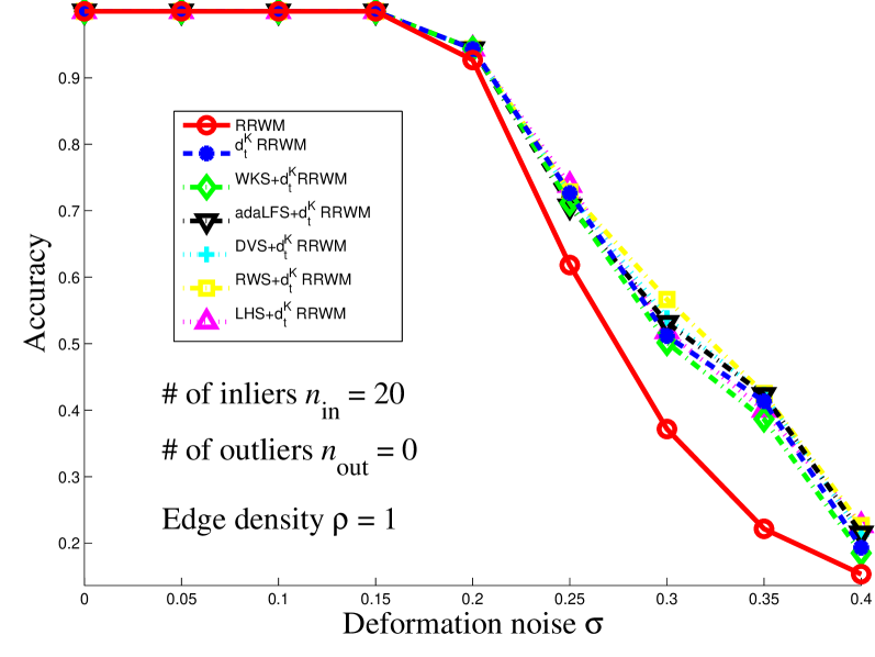
(a)

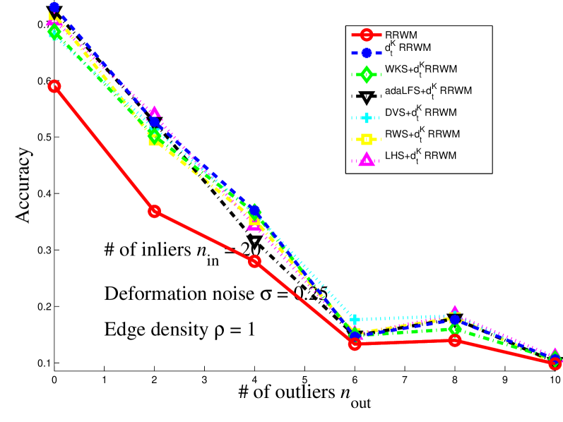
(b)

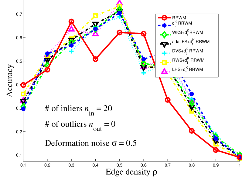
(c)

Figure 2: Matching accuracy of in the IQP setting.

Second, we test different node signatures together with $d_{t}^{{\cal K}}$ as the pairwise constraint in the IQP setting. The random graphs are generated according to [5] using their publicly available code. For a pair of graph $G_{1}$ and $G_{2}$, they share $n_{\text{in}}$ common nodes and $n_{\text{out}}^{(1)}$ and $n_{\text{out}}^{(2)}$ outlier nodes. Edge weights are randomly distributed in $[0,1]$, and random Gaussian noise ${\cal N}(0,\sigma^{2})$ is added.

In this experiment, we test the matching performance where the IQP compatibility matrix $W$ includes: i) only $d^{A}(i,j,a,b)$, ii) only $d_{t}^{{\cal K}}(i,j,a,b)$, iii) $d_{t}^{{\cal K}}(i,j,a,b)$ with different node signatures, on three different settings: 1. different level of deformation noise $\sigma$; 2. different number of outliers; 3. different edge densities $\rho$. Fig. 2 shows the average matching accuracy. The baseline, shown in red solid curve, is RRWM using pairwise adjacency distances $d^{A}$ only. With $d_{t}^{{\cal K}}$ substituting $d^{A}$, the matching performance is more tolerant to noise. Comparing Fig. 1(b) and Fig. 2(a), it can be seen that the large performance gap among node signatures, however, was marginalized out because of the second order compatibility constraint $d_{t}^{{\cal K}}$. As shown in Fig. 2, the matching accuracy of our proposed method is superior to the baseline algorithm (red solid line) in all three noisy settings.

6.2 CMU House Sequence

In this experiment, we use the CMU House sequence to test our descriptors. This sequence has been widely used to test different graph matching algorithms. It consists of 110 frames, and there are 30 feature points labeled consistently across all frames. We build fully connected graphs purely based on the geometry of the feature points, taking the exponential of the normalized Euclidean distance of the key points as the weights between pair of feature points. Note this graph setup is different from [5]. In their original work, they use the Euclidean distance as edge weights, which could be seen as a dissimilarity measure. While in our frame work, we used the normalized exponential of the dissimilarity as a similarity measure, which conforms with the physical meaning of neighboringness. IQP compatibility matrices $W$ are set up similarly as in Section 6.1. In the first part of the experiments, We compute the average matching accuracy of each frame to the rest of frames in the sequence. Fig. 1(c) shows the accuracy of the matching. As can be seen the matching performance improves when $d_{t}^{{\cal K}}$ is used to substitute $d^{A}$. With adaLFS as the first order compatibility, furthermore, the matching accuracy is improved even further. Fig. 3 shows an example of the matching between the first and the last frames of the sequence.

(a) RRWM

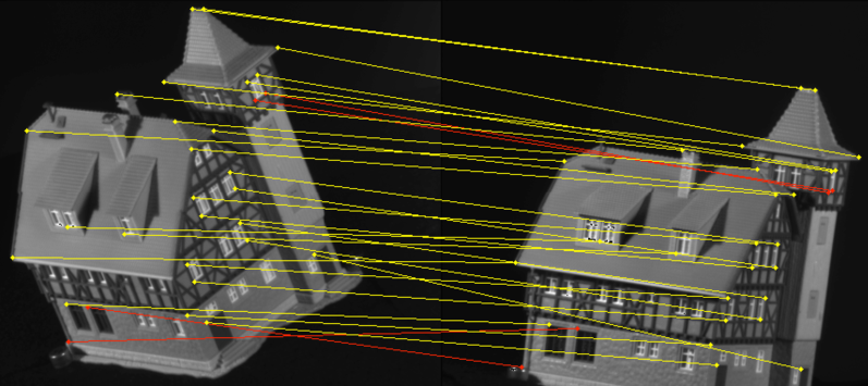
(b) WKS+$d_{t}^{{\cal K}}$ RRWM

(c) adaLFS+$d_{t}^{{\cal K}}$ RRWM

Figure 3: Example matching on House sequence. Yellow lines are correct matches, and red lines are incorrect matches.

In the second part of the experiments, we explore how outliers could potentially affect the performance of our matching framework. We follow the protocol in [5], by randomly select a subset of the nodes in one of the graphs in matching. Across the sequence, we match all possible image pairs, space by 10,20,30,40,50,60,70,80,90,100 frames, and compute the average matching accuracy.

Figure 4(a) and 4(b) show the matching performance for 25 and 20 randomly selected subset of nodes. It can be seen that with our optimized kernel and the proposed heat diffusion distance, our matching performance is greatly improved from the baseline RRWM algorithm. The matching results in their original work [5] using RRWM is better than our implementation of RRWM because they used a different graph structure in matching. The purpose of our comparison is to show the improvement from using our proposed first order and second order compatibilities with respect to the baseline adjacency matrix, while the construction of the adjacency matrices from images is outside the scope of our paper. The matching accuracy drops when the number of outliers increases (from 5 to 10), and when the gap increases. For smaller gaps with outliers, WKS has a negative effect on matching performance, because WKS has a relatively wide kernel hence more noise tolerant but less informative. In consequence, when the gaps are small, the smoothing WKS kernel instead of enhancing reduces the matching performance. On the contrary, it can be seen that our optimal kernel adapts to the different scenarios much better.

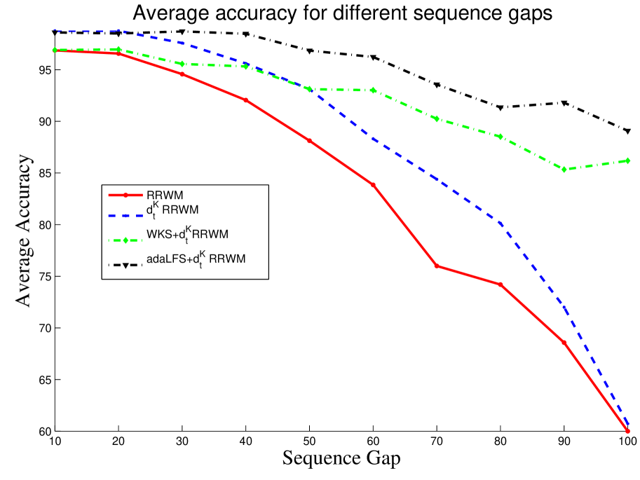
(a) 30 nodes to 25 nodes

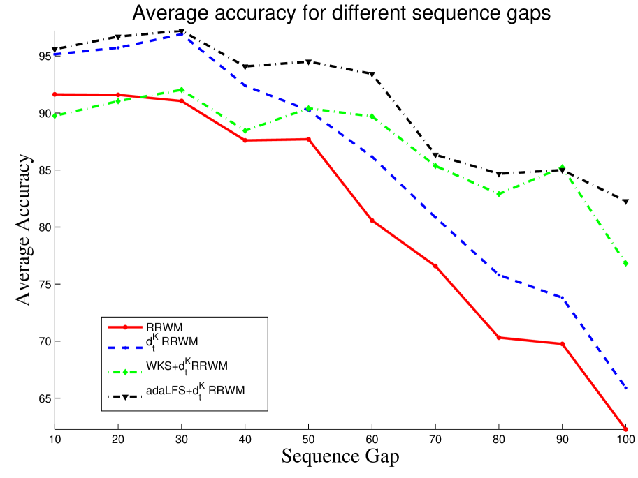
(b) 30 nodes to 20 nodes

Figure 4: Matching with random subset in House sequence.

6.3 Real Image Feature Matching

In this experiment, we test our descriptor on the real image dataset used in [5]. This image dataset consists of 30 pairs of images with labeled feature points. In their original paper, the IQP affinity matrix $W_{\text{feat}}$ was built considering the similarity between the appearance-based feature descriptors and the geometric transformations. Let $d_{\text{feat}}(i,j,a,b)$ be these compatibility functions from [5]. We add our spectral descriptors as additional structural compatibility, and set up the affinity matrix $W$ as

$$W_{ia,jb}=\begin{cases}d_{\text{feat}}(i,j,a,b)+\alpha d_{t}^{{\cal K}}(i,j,a,b)&i\neq j,~{}a\neq b\\ \beta d(i,a)&i=j,~{}a=b\end{cases}$$

This is done so that we can evaluate the effect of our structural descriptors on the matching results. In our experiments, we tested different combination of $\alpha$ and $\beta$. If only considering $d_{t}^{{\cal K}}$, $\alpha=1$, $\beta=0$ gives the best average accuracy, and by adding WKS/adaLFS as a node signature constraint, $\alpha=1,\beta=10$ gives the best average accuracy; Table 1 lists the average accuracies of different methods. Fig. 5 shows an example of matching results.

Table 1: Average accuracy of real image matching.

RRWM	$d_{t}^{{\cal K}}$	WKS+$d_{t}^{{\cal K}}$	adaLFS+$d_{t}^{{\cal K}}$
69.92	70.68	70.70	72.57

(a) RRWM (2/8)

(b) WKS+$d_{t}^{{\cal K}}$ (2/8)

(c) adaLFS+$d_{t}^{{\cal K}}$ (8/8)

Figure 5: Matching on real images.

7 Conclusion

In this paper, we considered the common quadratic assignment formulation of weighted graph matching problem, where we used LFS and the pairwise heat kernel distance as the first and second order compatibility terms. We have rigorously analyzed their stability properties; in the case of the first order terms we derived an objective function that measures both the stability and informativeness of a given spectral descriptor. By optimizing this objective, we designed new spectral node signatures tuned to a specific graph to be matched. Our experiments confirmed that these signatures outperform the existing spectral node signatures.

This work suggests a number of directions for future research. For exampe, instead of optimizing the signatures using solely the graph being matched, it would interesting to explore possibilities for computing representative graphs for graph collections arising in a given context. Another direction is to extend our constructions to higher order terms in the matching scheme [7, 4], or to use them for hypergraph matching [18].

References

- [1] Y. Aflalo, A. M. Bronstein, M. M. Bronstein, and R. Kimmel. Deformable shape retrieval by learning diffusion kernels. In SSVM’11, pages 689–700, 2011.
- [2] M. Aubry, U. Schlickewei, and D. Cremers. The wave kernel signature: A quantum mechanical approach to shape analysis. In ICCV - Workshop 4DMOD, 2011.
- [3] T. Biyikoglu, J. Leydold, and P. F. Stadler. Laplacian eigenvectors of graphs: Perron-Frobenius and Faber-Krahn Type Theorems. 2007.
- [4] M. Chertok and Y. Keller. Efficient high order matching. IEEE Transactions on PAMI, 32(12):2205 – 2215, 2010.
- [5] M. Cho, J. Lee, and K. M. Lee. Reweighted random walks for graph matching. In ECCV’10, pages 492–505, 2010.
- [6] T. Cour, P. Srinivasan, and J. Shi. Balanced graph matching. In NIPS’06, pages 313–320, 2006.
- [7] O. Duchenne, F. Bach, I. Kweon, and J. Ponce. A tensor-based algorithm for high-order graph matching. CVPR, pages 1980 – 1987, 2009.
- [8] A. Egozi, Y. Keller, and H. Guterman. A probabilistic approach to spectral graph matching. IEEE Transactions on PAMI, 99(PrePrints), 2012.
- [9] D. Emms, R. C. Wilson, and E. R. Hancock. Graph matching using the interference of continuous-time quantum walks. Pattern Recogn., 42(5):985–1002, May 2009.
- [10] M. Eshera and K. Fu. A graph distance measure for image analysis. IEEE Trans. Syst. Man Cybern., pages 398–408, 1984.
- [11] S. Gold and A. Rangarajan. A graduated assignment algorithm for graph matching. IEEE Trans. Patt. Anal. Mach. Intell., 18, 1996.
- [12] M. Gori, M. Maggini, and L. Sarti. Exact and approximate graph matching using random walks. IEEE Trans. Pattern Anal. Mach. Intell., 27(7):1100–1111, July 2005.
- [13] D. K. Hammond, P. Vandergheynst, and R. Gribonval. Wavelets on graphs via spectral graph theory. Applied and Computational Harmonic Analysis, 30(2):129–150, Mar. 2011.
- [14] N. Hu and L. Guibas. Spectral descriptors for graph matching. arXiv:1304.1572, 2013.
- [15] N. Hu, R. Rustamov, and L. Guibas. Graph matching with anchor nodes: A learning approach. CVPR, 2013.
- [16] S. Jouili and S. Tabbone. Graph matching based on node signatures. In GbRPR ’09, pages 154–163, 2009.
- [17] H. Kuhn. The hungarian method for the assignment problem. Naval Research Logistic Quarterly, pages 83 – 97, 1955.
- [18] J. Lee, M. Cho, and K. M. Lee. Hyper-graph matching via reweighted random walks. CVPR, pages 1633 – 1640, 2011.
- [19] M. Leordeanu and M. Hebert. A spectral technique for correspondence problems using pairwise constraints. In ICCV ’05, volume 2, pages 1482–1489, 2005.
- [20] M. Leordeanu, M. Hebert, and R. Sukthankar. An integer projected fixed point method for graph matching and map inference. In Proceedings NIPS, December 2009.
- [21] R. Litman and A. M. Bronstein. Learning spectral descriptors for deformable shape correspondence. IEEE Transactions on PAMI, 99(PrePrints):1, 2013.
- [22] B. Luo and E. R. Hancock. Structural graph matching using the em algorithm and singular value decomposition. IEEE Trans. PAMI, 23(10):1120–1136, Oct. 2001.
- [23] M. Newman. Networks, An Introduction. 2010.
- [24] H. Qiu and E. R. Hancock. Graph matching and clustering using spectral partitions. Pattern Recogn., 39(1):22–34, Jan. 2006.
- [25] A. Robles-Kelly and E. R. Hancock. String edit distance, random walks and graph matching. In Joint IAPR International Workshop SSSPR, pages 104–112, 2002.
- [26] A. Robles-Kelly and E. R. Hancock. Graph edit distance from spectral seriation. IEEE Trans. Pattern Anal. Mach. Intell., 27(3):365–378, Mar. 2005.
- [27] C. Schellewald and C. Schnörr. Probabilistic subgraph matching based on convex relaxation. In EMMCVPR’05, pages 171–186, 2005.
- [28] A. Shokoufandeh and S. Dickinson. Applications of bipartite matching to problems in object recognition. Proceedings, ICCV Workshop on Graph Algorithms and Computer Vision, September 1999.
- [29] A. Shokoufandeh and S. J. Dickinson. A unified framework for indexing and matching hierarchical shape structures. In Proceedings of IWVF-4, pages 67–84, 2001.
- [30] J. Sun, M. Ovsjanikov, and L. Guibas. A concise and provably informative multi-scale signature based on heat diffusion. In SGP, 2009.
- [31] S. Umeyama. An eigendecomposition approach to weighted graph matching problems. IEEE Trans. PAMI, 10(5):695–703, 1988.
- [32] B. J. van Wyk and M. A. van Wyk. A pocs-based graph matching algorithm. IEEE Trans. PAMI, 26(11):1526–1530, Nov. 2004.
- [33] R. C. Wilson and P. Zhu. A study of graph spectra for comparing graphs and trees. Pattern Recogn., 41(9):2833–2841, Sept. 2008.
- [34] P. C. Wong, H. Foote, G. Chin, P. Mackey, and K. Perrine. Graph signatures for visual analytics. IEEE Trans Vis Comput Graph, 12(6):1399–413, 2006.
- [35] M. Zaslavskiy, F. Bach, and J.-P. Vert. A path following algorithm for the graph matching problem. IEEE Trans on PAMI, 31(12):2227–2242, 2009.
- [36] R. Zass and A. Shashua. Probabilistic graph and hypergraph matching. CVPR, 2008.
- [37] G. Zhao, B. Luo, J. Tang, and J. Ma. Using eigen-decomposition method for weighted graph matching. In ICIC’07, pages 1283–1294, 2007.
- [38] F. Zhou and F. De la Torre. Factorized graph matching. CVPR, pages 127 – 134, 2012.