A STUDY OF TRANSIT TIMES IN DIRAC TUNNELLING

Abstract

Based on the Dirac equation, the behavior of relativistic electrons which tunnel a potential barrier of height $V_{\mbox{\tiny$0$}}$ for incoming energies between $V_{\mbox{\tiny$0$}}$ and $V_{\mbox{\tiny$0$}}+m$ is studied by using the wave packet formalism. The choice of this incoming energy zone guarantees that only electrons participate to the tunneling process. In the opaque limit, as shown in a previous analysis, the transit velocity is proportional to the barrier width and for relativistic potential tends to a constant value greater than $c$. In this paper, a new numerical study shows a very surprising result: superluminal transmissions are also evident for thin barriers.

I. INTRODUCTION

In this paper, by using the Dirac equation, we examine the relationship between the peak of the incoming wave packet (of energy $E$ and mass $m$) which encounters a potential barrier of height $V_{\mbox{\tiny$0$}}$ and width $L$ at $z=0$ and the peak of transmitted wave packet which moves in the free potential region after the barrier. The terminology “Dirac tunneling” refers to the energy zone of the incoming particles, $V_{\mbox{\tiny$0$}}<E<V_{\mbox{\tiny$0$}}+m$[1, 2, 3]. This energy zone is characterized by evanescent solutions in the region $0<z<L$, i.e. $\exp[\pm\,\rho\,z]$ with $\rho=\sqrt{m^{\mbox{\tiny$2$}}-(E-V_{\mbox{\tiny$0$}})^{{}^{2}}}$. The terminology Dirac tunneling is useful to distinguish these evanescent solutions form the evanescent solutions which appear in the Klein tunneling zone, $V_{\mbox{\tiny$0$}}-m<E<V_{\mbox{\tiny$0$}}$[3]. The study of the Klein tunneling zone exceeds the scope of this paper and it will be appropriately discussed in a forthcoming article. It is important to observe that the Klein tunneling zone has not to be confused with the standard Klein zone, $E<V_{\mbox{\tiny$0$}}-m$, which is characterized by oscillating antiparticle solutions, i.e. $\exp[\pm\,i\,q\,z]$ with $q=\sqrt{(E-V_{\mbox{\tiny$0$}})^{{}^{2}}-m^{\mbox{\tiny$2$}}}$ and the appearance of the Klein paradox[4, 5, 6, 7]. For the convenience of the reader, we draw the energy Dirac/Klein zones in the following picture

The incoming electrons will be described by a wave packet with a gaussian momentum distribution, $g(p)$ centered at $p_{\mbox{\tiny$0$}}$,

$$g(p)=\left\{\begin{array}[]{ll}\exp\left[\,-\,(p-p_{\mbox{\tiny$0$}})^{{}^{2}}d^{{}^{2}}\,/\,4\,\right]&\,\,\,\mbox{for}\,\,\,\,\,\sqrt{V_{\mbox{\tiny$0$}}^{{}^{2}}-m_{e}^{\mbox{\tiny$2$}}}=p_{\mbox{\tiny$min$}}\leq\,p\,\leq p_{\mbox{\tiny$max$}}=\sqrt{V_{\mbox{\tiny$0$}}(V_{\mbox{\tiny$0$}}+2m_{e})}\,\,,\\ \\ 0&\,\,\,\mbox{otherwise}\,\,,\end{array}\right.$$

where the minimum and maximum values of the momentum distribution are chosen to guarantee Dirac tunneling. The barrier filter effect modifies the incoming momentum distribution[8, 9, 10, 11]. The momentum mean value $p_{\mbox{\tiny$0$}}$ after transmission tends to an higher value, say $p_{\mbox{\tiny$L$}}$. In the opaque limit ($m_{e}L\gg 1$) $p_{\mbox{\tiny$L$}}\approx p_{\mbox{\tiny$max$}}$. For thin barriers $p_{\mbox{\tiny$L$}}\approx p_{\mbox{\tiny$0$}}$. The incoming electrons move in the free region before the barrier with a subluminal velocity given by $v_{\mbox{\tiny$0$}}=p_{\mbox{\tiny$0$}}/E_{\mbox{\tiny$0$}}$. The outgoing electrons move in the free region after the barrier with a greater, but obviously still subluminal, velocity $v_{\mbox{\tiny$L$}}=p_{\mbox{\tiny$L$}}/E_{\mbox{\tiny$L$}}$. This implies that the maximum of the spatial distribution of electrons, which tunnels a barrier of width $L$, will reach the position $D>L$ at time

$$t_{\mbox{\tiny$D$},\mbox{\tiny$L$}}=\frac{L}{v_{\mbox{\tiny$tun$}}}\,+\frac{D-L}{v_{\mbox{\tiny$L$}}}\,\,.$$ (1)

A natural question is to ask if and in which cases the average velocity $v_{\mbox{\tiny$D$},\mbox{\tiny$L$}}=D/\,t_{\mbox{\tiny$L$}}$ is superluminal. Our paper was intended as an attempt to give a satisfactory answer to this intriguing question not only in the opaque limit, where the transmission probability goes to zero, but also for thinner barriers, where greater transmission probabilities are found. Finally, the choice of the Dirac tunneling energy zone seems to be the more appropriate in discussing superluminal velocities because it avoids the possibility that the electrons which appear in the free potential region after the barrier are products of pairs production (a typical phenomenon of the Klein zone). The lower limit ($V_{\mbox{\tiny$0$}}<m$) is not covered in this work.

II. THE DIRAC EQUATION IN PRESENCE OF A POTENTIAL BARRIER

Since we shall need the solutions for a barrier potential, we rewrite the free Dirac equation

$$i\,\gamma^{\mu}\partial_{\mu}\Psi(\boldsymbol{r},t)=m_{e}\,\Psi(\boldsymbol{r},t)\,\,,$$ (2)

by including, via minimal coupling $\partial_{\mu}\to\partial_{\mu}-i\,e\,A_{\mu}$[12, 13], an electrostatic potential $A_{\mu}=\left[A(z)\,,\,\boldsymbol{0}\right]$, where $A(z)=A_{\mbox{\tiny$0$}}$ for $0<z<L$ and $0$ otherwise,

$$\left[\,i\,\gamma^{\mu}\partial_{\mu}+e\,\gamma_{\mbox{\tiny$0$}}A(z)\,\right]\Psi(\boldsymbol{r},t)=m_{e}\,\Psi(\boldsymbol{r},t)\,\,.$$ (3)

Considering a one-dimensional motion, $p_{x}=p_{y}=0$ and $p_{z}=p$, and stationary state solutions, $\psi(z)\exp[\,-\,i\,E\,t)]$, we obtain

$$\gamma_{\mbox{\tiny$0$}}\left[\,E-V(z)\,\right]\,\psi(z)+i\,\gamma_{\mbox{\tiny$3$}}\,\psi^{\prime}(z)=m_{e}\,\psi(z)\,\,,$$ (4)

where $V(z)=-eA(z)$ and the prime indicates the derivative with respect to $z$. In any constant potential region, for a given $E$, only two solutions exist be they oscillatory ($|E-V_{\mbox{\tiny$0$}}|>m$) or evanescent ($|E-V_{\mbox{\tiny$0$}}|<m$). Using the Pauli-Dirac set of gamma matrices and observing that for one-dimensional phenomena spin flip does not occur, we find, for Dirac tunneling, the following spinorial solutions[3]

$$\begin{array}[]{lcl}\mbox{\sc Region I}&\,\,\,:&u(p\,,\,E)\,\,e^{+\,i\,p\,z}+R\,\,u(-p\,,\,E)\,\,e^{-\,i\,p\,z}\,\,,\\ \mbox{\sc Region II}&\,\,\,:&A\,\,u(i\,\rho\,,\,E-V_{\mbox{\tiny$0$}})\,\,e^{-\,\rho\,z}+B\,\,u(-\,i\,\rho\,,\,E-V_{\mbox{\tiny$0$}})\,\,e^{+\,\rho\,z}\,\,,\\ \mbox{\sc Region III}&\,\,\,:&T\,\,u(p\,,\,E)\,\,e^{+\,i\,p\,z}\,\,,\end{array}$$ (5)

where

$$u(p\,,\,E)=\left[\,1\,,\,0\,,\,p\,/(E+m_{e})\,,\,0\,\right]^{t}\,\,.$$

Because the Dirac equation is a first order equation in the spatial derivatives, for a step-wise continuous potential, only the continuity of the wave function has to be required. Imposing the continuity conditions, $\psi_{\mbox{\tiny$I$}}(0)=\psi_{\mbox{\tiny$II$}}(0)$ and $\psi_{\mbox{\tiny$II$}}(L)=\psi_{\mbox{\tiny$III$}}(L)$, we obtain the following transmission coefficient

$$T(p,L)=e^{-\,i\,p\,L}\,\mbox{\Large$/$}\,\left[\,\cosh(\,\rho L)\,-\,i\,\,\frac{p^{\mbox{\tiny$2$}}-V_{\mbox{\tiny$0$}}E}{p\,\rho}\,\sinh(\,\rho L)\right]\,\,.$$ (6)

The transmitted wave packet is then obtained by integrating over all the possible stationary states modulated by the weighting function $g(p)$,

$$\Psi_{\mbox{\tiny$T$}}(z,t) = \int_{p_{\mbox{\tiny$min$}}}^{p_{{max}}}\,\mbox{d}p\,\,g(p)\,T(p,L)\,u(p,E)\,\,e^{i\,[\,p\,z-E\,t\,]}$$ (7)

$$= \int_{p_{\mbox{\tiny$min$}}}^{p_{{max}}}\,\mbox{d}p\,\left[\,g_{\mbox{\tiny$T$}}(p,L)\,,\,0\,,\,f_{\mbox{\tiny$T$}}(p,L)\,,\,0\,\right]^{t}\,\,e^{i\,\theta}\,\,e^{i\,[\,p\,(z-L)-E\,t\,]}\,\,,$$

where

$$\tan\theta=\frac{p^{\mbox{\tiny$2$}}-V_{\mbox{\tiny$0$}}E}{p\,\rho}\,\tanh(\rho L)\,\,\,,\,\,\,\,\,\,\,g_{\mbox{\tiny$T$}}(p,L)=g(p)\,\,|T(p,L)|\,\,\,\,\,\,\,\mbox{and}\,\,\,\,\,\,\,f_{\mbox{\tiny$T$}}(p,L)=\frac{p}{E+m_{e}}\,\,g_{\mbox{\tiny$T$}}(p,L)\,\,.$$

III. THE FILTER EFFECT FOR OPAQUE BARRIERS

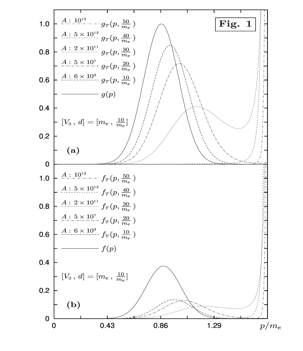
Figure 1: Momentum distributions for the up, $g_{\mbox{\tiny$T$}}(p,L)$, and down, $f_{\mbox{\tiny$T$}}(p,L)$, component of the transmitted Dirac spinors. The incoming momentum distribution $g(p)$ is centered at $p_{\mbox{\tiny$0$}}=\sqrt{3}\,m_{e}/2$. Its space localization is determined by $d=10/m_{e}$. By increasing the value of the barrier width $L$, the filter effect modifies the initial momentum distributions leading, for $m_{e}L\gg 1$, to smaller transmission probabilities, to greater momentum mean values, $p_{\mbox{\tiny$L$}}\to p_{\mbox{\tiny$max$}}$, and to localizations $\gg d$.

This section contains a brief summary of the discussion recently appeared in literature[14] on the filter effect for opaque barriers in the Dirac equation. The action of the filter effect[8] on the momentum distribution of the transmitted wave, $g_{\mbox{\tiny$T$}}(p,L)$ and $f_{\mbox{\tiny$T$}}(p,L)$, is shown in Fig. 1. For increasing values of the barrier width $L$, the transmitted momentum averaged over the distributions $g_{\mbox{\tiny$T$}}(p,L)$ and $f_{\mbox{\tiny$T$}}(p,L)$,

$$p_{\mbox{\tiny$L$}}:=\langle p\rangle_{\mbox{\tiny$T$}}=\int_{p_{\mbox{\tiny$min$}}}^{p_{{max}}}\,\mbox{d}p\,p\,\left[\,g^{\mbox{\tiny$2$}}_{\mbox{\tiny$T$}}(p,L)+f^{{}^{2}}_{\mbox{\tiny$T$}}(p,L)\right]\,\mbox{\huge/}\,\int_{p_{\mbox{\tiny$min$}}}^{p_{{max}}}\,\mbox{d}p\,\left[\,g^{\mbox{\tiny$2$}}_{\mbox{\tiny$T$}}(p,L)+f^{{}^{2}}_{\mbox{\tiny$T$}}(p,L)\right]\,\,,$$ (8)

tends to $p_{\mbox{\tiny$max$}}$. This splitting of the average momentum is due to the higher momenta selection caused by the exponential functional dependence, $\exp[-\rho L]$, of the transmission coefficient $T(p,L)$. The plots in Fig. 1 refer to a potential barrier of height $V_{\mbox{\tiny$0$}}=m_{e}$, which implies $p_{\mbox{\tiny$min$}}=0$ and $p_{\mbox{\tiny$max$}}=\sqrt{3}\,m_{e}$, and an incoming momentum $p_{\mbox{\tiny$0$}}=\sqrt{3}\,m_{e}/2$. The space localization for the incoming wave packet is determined by $m_{e}d=10$. The ratio between the down and up distribution, as a consequence of the higher momenta filter, increases from $p_{\mbox{\tiny$0$}}/(E_{\mbox{\tiny$0$}}+m_{e})\approx 37.3\%$ to $p_{\mbox{\tiny$max$}}/(E_{max}+m_{e})\approx 57.7\%$.

Without going into the details of the mathematical apparatus of asymptotic integral expansions and, in particular, of the validity and possible generalization of the stationary phase method which find a complete description in a number of books[15, 16] and papers[8, 9, 10, 11], we briefly discuss the case of opaque barriers, i.e. $m_{e}L\gg 1$. In this limit, the cosh and sinh functions with argument $\rho L$ can be approximated by $\exp[-\rho L]/2$. This allows to rewrite the transmitted coefficient as

$$|T(p,m_{e}L\gg 1)|\approx 2\,p\,\rho\,e^{-\,\rho\,L}\,/\,m_{e}V_{\mbox{\tiny$0$}}\,\,.$$ (9)

Now, the computation of the integral given in Eq. (7), taking into account the previous approximation, can be done analytically. Starting from

$$||\Psi_{\mbox{\tiny$T$}}(L,t;m_{e}L\gg 1)\,||\approx\frac{2}{m_{e}V_{\mbox{\tiny$0$}}}\,\,g(p_{\mbox{\tiny$max$}})\,\sqrt{\frac{2\,E_{\mbox{\tiny$max$}}}{E_{\mbox{\tiny$max$}}+m_{e}}}\,\,\,\left|\,\int_{p_{\mbox{\tiny$min$}}}^{p_{\mbox{\tiny$max$}}}\,\mbox{d}p\,\,p\,\rho\,\,\,e^{-\,\rho\,L}\,e^{i\,(\theta-E\,t)}\right|\,\,,$$ (10)

changing the variable of integration from $p$ to $\rho$,

$$p\,\mbox{d}p\approx-\,\frac{E_{max}}{V_{\mbox{\tiny$0$}}-E_{max}}\,\rho\,\mbox{d}\rho\,\,\,,\,\,\,\,\,\,\,\rho(p_{\mbox{\tiny$min$}})=m_{e}\,\,\,\,\,\mbox{and}\,\,\,\,\,\rho(p_{\mbox{\tiny$max$}})=0\,\,,$$

and using the following series expansions for $\theta$ and $E$,

$$\theta\approx\theta_{\mbox{\tiny$max$}}-\,a_{\mbox{\tiny$1$}}\,\rho\,+\,\mbox{O}[\,\rho^{\mbox{\tiny$3$}}]\,\,\,\,\,\mbox{and}\,\,\,\,\,E=E_{\mbox{\tiny$max$}}-\,a_{\mbox{\tiny$2$}}\,\rho^{\mbox{\tiny$2$}}\,+\,\mbox{O}[\,\rho^{\mbox{\tiny$4$}}]\,\,,$$

where $a_{\mbox{\tiny$1$}}=\sqrt{V_{\mbox{\tiny$0$}}(V_{\mbox{\tiny$0$}}+2\,m_{e})}\,/m_{e}V_{\mbox{\tiny$0$}}$ and $a_{\mbox{\tiny$2$}}=1/2m_{e}$, we find

$$||\Psi_{\mbox{\tiny$T$}}(L,t;m_{e}L\gg 1)\,|| \propto \left|\,\int_{0}^{m_{e}}\,\mbox{d}\rho\,\,\rho^{\mbox{\tiny$2$}}\,e^{-\,\rho L}\,\,\exp\left[\,i\,\left(\,a_{\mbox{\tiny$2$}}t\,\rho^{\mbox{\tiny$2$}}-\,a_{\mbox{\tiny$1$}}\,\rho\,\right)\right]\right|$$ (11)

$$\approx \left|\,\int_{0}^{m_{e}}\,\mbox{d}\rho\,\,\rho^{\mbox{\tiny$2$}}\,e^{-\,\rho L}\,\,\left[\,1+i\,\left(\,a_{\mbox{\tiny$2$}}t\,\rho^{\mbox{\tiny$2$}}-a_{\mbox{\tiny$1$}}\,\rho\,\right)-\left(\,a_{\mbox{\tiny$2$}}t\,\rho^{\mbox{\tiny$2$}}-a_{\mbox{\tiny$1$}}\,\rho\,\right)^{{}^{2}}/\,2\right]\right|\,\,.$$

It is clear from this discussion that the problem of finding the maximum of the transmitted wave packet reduces, in the opaque barrier limit, to find the maximum of the function

$$\mathcal{P}_{\mbox{\tiny$T$}}(t)=\left|\,s(2)-\left[(a_{\mbox{\tiny$2$}}t)^{\mbox{\tiny$2$}}\,s(6)+a_{\mbox{\tiny$1$}}^{\mbox{\tiny$2$}}s(4)\right]/\,2+a_{\mbox{\tiny$1$}}a_{\mbox{\tiny$2$}}t\,s(5)+i\,\left[a_{\mbox{\tiny$2$}}t\,s(4)-a_{\mbox{\tiny$1$}}s(3)\right]\,\right|^{{}^{2}}\,\,,$$ (12)

where

$$s(n)=\int_{\mbox{\tiny$0$}}^{m_{e}}\,\mbox{d}\rho\,\rho^{n}\,e^{-\,\rho L}\approx\,\,n!\,/\,L^{{}^{n+1}}\,\,.$$

The condition $\partial_{t}||\Psi_{\mbox{\tiny$T$}}(L,t;m_{e}L\gg 1)||^{{}^{2}}=0$ is thus satisfied requiring $\mathcal{P}_{\mbox{\tiny$T$}}^{\prime}(t)=0$. Observing that

$$\mathcal{P}_{\mbox{\tiny$T$}}(t)\approx s^{\mbox{\tiny$2$}}(2)+a_{\mbox{\tiny$1$}}^{\mbox{\tiny$2$}}\,[\,s^{\mbox{\tiny$2$}}(3)-s(2)s(4)\,]+2\,a_{\mbox{\tiny$1$}}a_{\mbox{\tiny$2$}}t\,[\,s(2)s(5)-s(3)s(4)\,]+(a_{\mbox{\tiny$2$}}t)^{\mbox{\tiny$2$}}[\,s^{\mbox{\tiny$2$}}(4)-s(2)s(6)\,]\,\,,$$

we find for the tunneling time, $\tau_{\mbox{\tiny$tun$}}$, the following equation

$$a_{\mbox{\tiny$1$}}[\underbrace{s(2)s(5)-s(3)s(4)}_{4\,\cdot\,4!\,/\,L^{{}^{9}}}]+\,a_{\mbox{\tiny$2$}}\tau_{\mbox{\tiny$tun$}}\,[\underbrace{s^{\mbox{\tiny$2$}}(4)-s(2)s(6)}_{-\,36\,\cdot\,4!\,/\,L^{{}^{10}}}]=0\,\,.$$ (13)

From this equation, we obtain a closed formula for the tunneling velocity,

$$v_{\mbox{\tiny$tun$}}=\frac{L}{\tau_{\mbox{\tiny$tun$}}}=\frac{9\,a_{\mbox{\tiny$2$}}}{a_{\mbox{\tiny$1$}}}=\,\frac{9}{2}\,\sqrt{\frac{V_{\mbox{\tiny$0$}}}{V_{\mbox{\tiny$0$}}+2\,m_{e}}}\,\,.$$ (14)

In order to understand the importance of Eq. (14), let us present two limit cases. For non relativistic potentials,

$$v_{\mbox{\tiny$tun$}}[V_{\mbox{\tiny$0$}}\ll m_{e}]\approx\frac{9}{2}\,\sqrt{\frac{V_{\mbox{\tiny$0$}}}{2\,m_{e}}}\ll 1\,\,.$$

This means that the use the Schrödinger equation leads to non-relativistic tunneling velocities. A surprising result is seen in the chiral limit,

$$v_{\mbox{\tiny$tun$}}[V_{\mbox{\tiny$0$}}\gg m_{e}]\approx\frac{9}{2}\,\,,$$

where superluminal tunneling velocities appear[14].

IV. NUMERICAL ANALYSIS AND TRANSIT TIMES

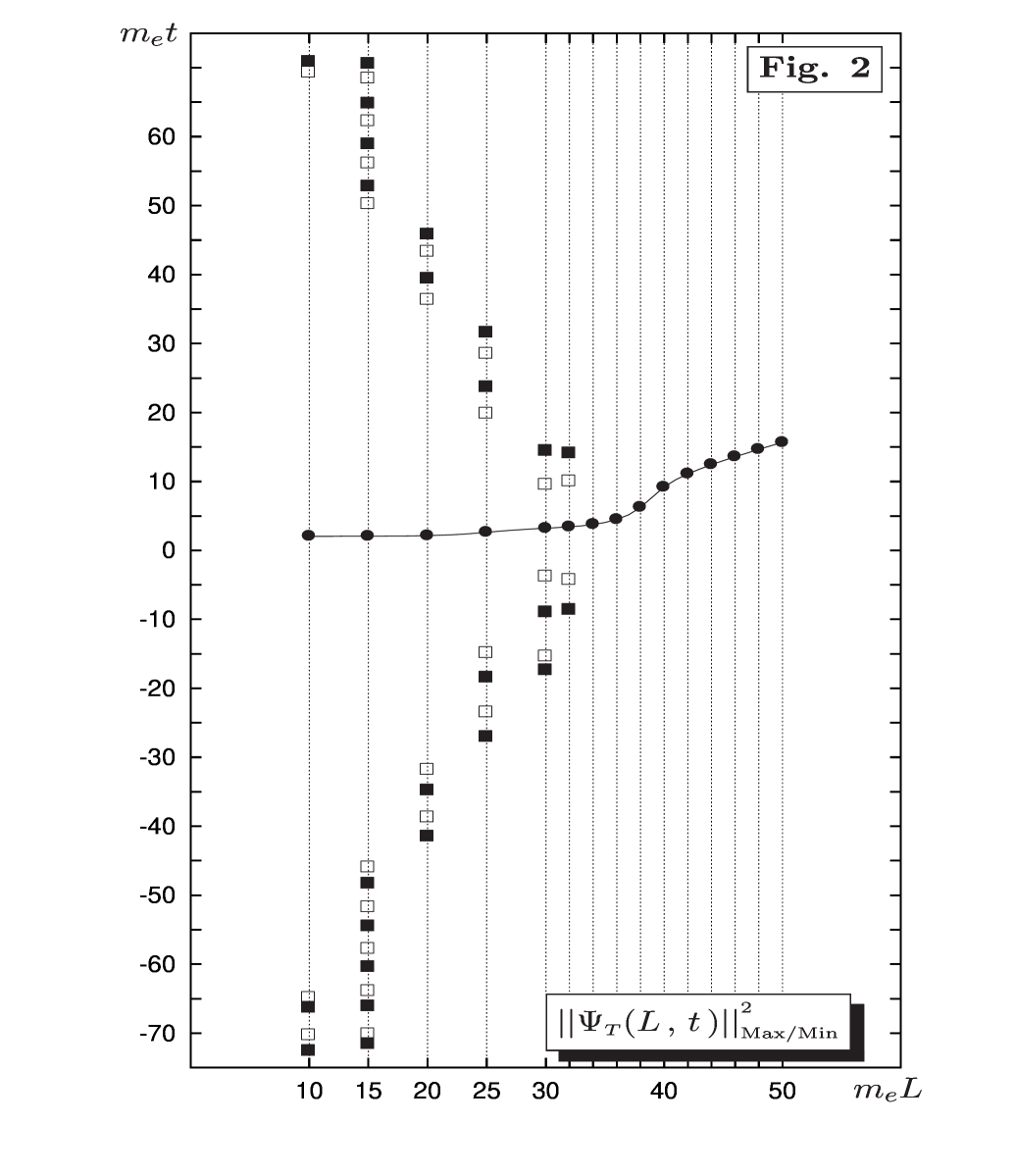
Figure 2: Maximum and minimum values of the transmitted probability density at $z=L$ in correspondence to the time in which it appears in the free region after the barrier. The black circles indicates the central peak. The secondary peaks are identified by the black squares. Finally, the white squares represent the times in which the minima appear in $z=L$. The numerical data refer to incoming electrons, with a momentum distribution centered at $p_{\mbox{\tiny$0$}}=\sqrt{3}\,m_{e}/2$ and localization determined by $d=10/m_{e}$, which tunnel a potential barrier of height $V_{\mbox{\tiny$0$}}=m_{e}$ and width $L$.

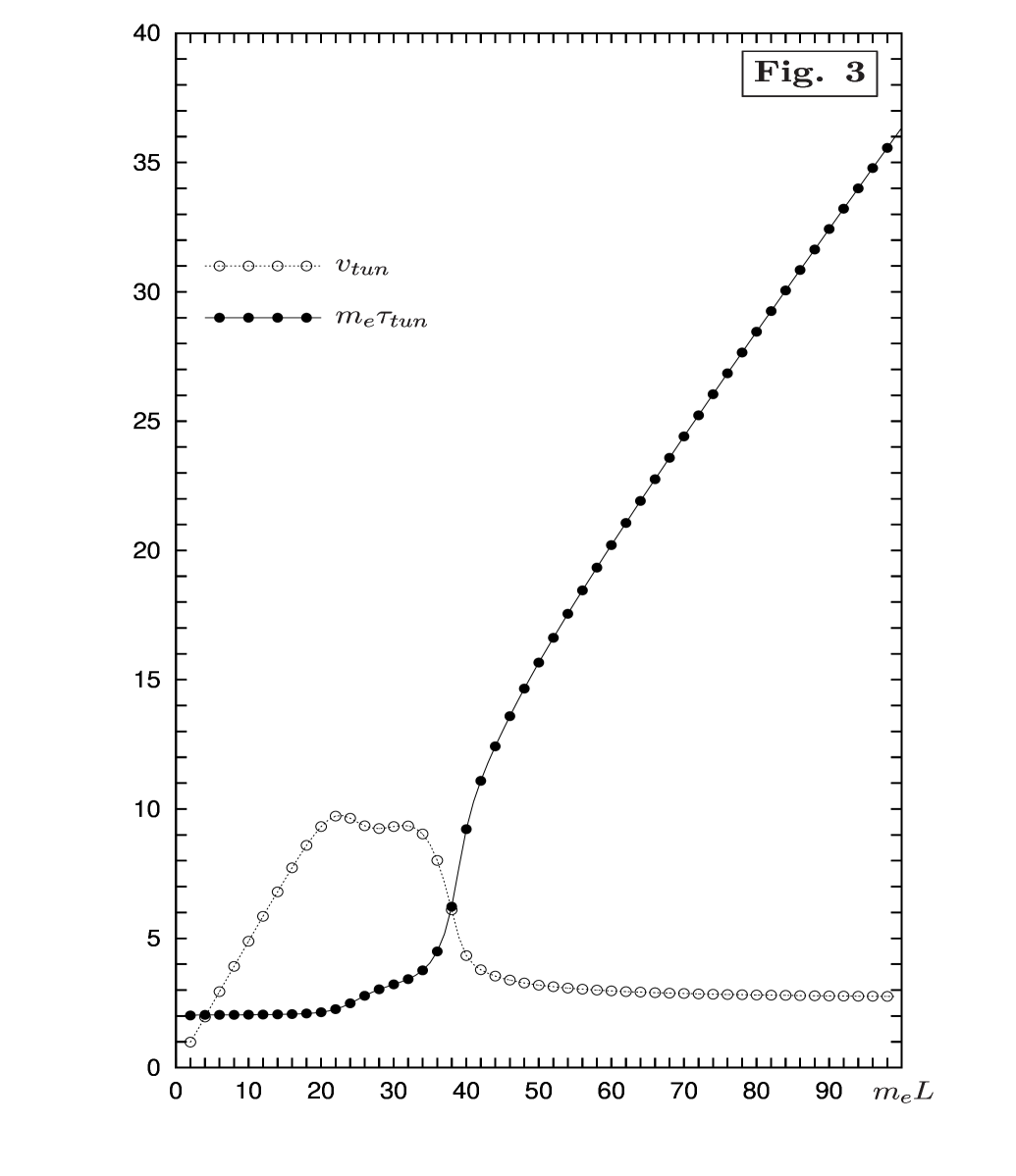
Figure 3: Tunneling times (black circles and continuous line) and tunneling velocity (withe circles and dotted line) for incoming electrons of momentum $p_{\mbox{\tiny$0$}}=\sqrt{3}\,m_{e}/2$ and localization $d=10/m_{e}$ which tunnel a potential barrier of height $V_{\mbox{\tiny$0$}}=m_{e}$ and width $L$. The numerical data confirm the analytic formula obtained in the opaque limit for the tunneling velocity, see Eq. (14). An unexpected and surprising result is seen for thin barriers ($\approx 2\,d$) where the superluminal tunneling velocity reaches its maximum value ($\approx 10$).

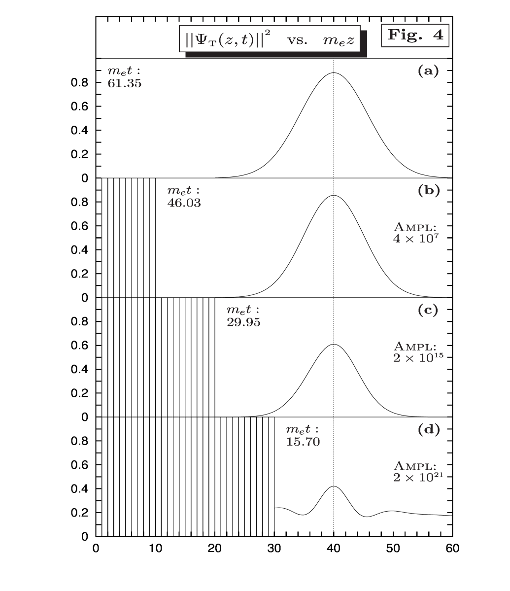
Figure 4: Probability density for incoming electrons, with a momentum distribution centered at $p_{\mbox{\tiny$0$}}=\sqrt{3}\,m_{e}/2$ and localization $d=10/m_{e}$, which move in free space (a), tunnel a potential barrier of width $L$ equal to $10/m_{e}$ (b), $20/m_{e}$ (c), and $30/m_{e}$ (d). In the free space the electrons move with a mean velocity $v_{\mbox{\tiny$4$}\mbox{\tiny$0$},\mbox{\tiny$0$}}\approx 0.65$. Barrier tunneling increases the velocity of propagation leading to superluminal transmission, $v_{\mbox{\tiny$4$}\mbox{\tiny$0$},\mbox{\tiny$2$}\mbox{\tiny$0$}}\approx 1.34$ and $v_{\mbox{\tiny$4$}\mbox{\tiny$0$},\mbox{\tiny$3$}\mbox{\tiny$0$}}\approx 2.55$.

Up to this point, we have limited ourselves to a strictly analytic approach to the problem. To test our analysis, we have performed a numerical study by using Mathematica 8 [Wolfram] whose results are shown in Fig. 2 and Fig. 3. The numerical analysis shows the phenomenon of multiple peaks. The spatial distribution of these peaks is plotted in Fig. 2 for a barrier of height $V_{\mbox{\tiny$0$}}=m_{e}$ and incoming momentum distribution centered to $p_{\mbox{\tiny$0$}}=\sqrt{3}\,m_{e}/\,2$. In Table 1, we give the values of the transmitted probability density and the corresponding appearance time for the first peaks around the main maximum. For thinner barrier the secondary peaks are very small when compared to the main peak. The phenomenon of multiple peaks disappears for increasing values of the barrier width. In Fig. 3, we show the barrier width dependence of the tunneling time, $\tau_{\mbox{\tiny$tun$}}$, referring to the main peak and the corresponding tunneling velocity, $v_{\mbox{\tiny$tun$}}$. The analytic value of the tunneling velocity, calculated by using Eq. (14) for $V_{\mbox{\tiny$0$}}=m_{e}$, $9/2\sqrt{3}$, is in good agreement with the numerical data. The important point to be noted here is that the numerical data clearly show superluminal tunneling velocities also for thinner barriers, see Fig. 3 in the initial range of the barrier width. The conclusion of our numerical study is unexpected and quite surprising. For thinner barrier superluminal tunneling velocities appear and the superluminal effects are greater than those observed in the opaque barrier limit. Due to this surprising result, we have investigated in details the behavior of an incoming wave packet of momentum $p_{\mbox{\tiny$0$}}=\sqrt{3}\,m_{e}/\,2$ and localization $d=10/m_{e}$ which starting from the point $z=0$ at time $t=0$ reaches the point $D=40/m_{e}$ travelling through free space (Fig. 4a), tunneling a barrier of width $L=10/m_{e}$ (Fig. 4b), a barrier of width $L=20/m_{e}$ (Fig. 4c), and a barrier of width $L=30/m_{e}$ (Fig. 4d). The transmitted peak is found at $D=40/m_{e}$ at the following times, $\{t_{\mbox{\tiny$D$},\mbox{\tiny$L$}}\}$,

$$\left\{\,m_{e}\,t_{\mbox{\tiny$4$}\mbox{\tiny$0$},\mbox{\tiny$0$}}\,,\,m_{e}\,t_{\mbox{\tiny$4$}\mbox{\tiny$0$},\mbox{\tiny$1$}\mbox{\tiny$0$}}\,,\,m_{e}\,t_{\mbox{\tiny$4$}\mbox{\tiny$0$},\mbox{\tiny$2$}\mbox{\tiny$0$}}\,,\,m_{e}\,t_{\mbox{\tiny$4$}\mbox{\tiny$0$},\mbox{\tiny$3$}\mbox{\tiny$0$}}\,\right\}=\left\{\,61.35\,,\,46.03\,,\,29.95\,,\,15.70\,\right\}\,\,.$$

These numerical times imply the following transit velocities, $\{v_{\mbox{\tiny$D$},\mbox{\tiny$L$}}\}$,

$$\left\{\,v_{\mbox{\tiny$4$}\mbox{\tiny$0$},\mbox{\tiny$0$}}\,,\,v_{\mbox{\tiny$4$}\mbox{\tiny$0$},\mbox{\tiny$1$}\mbox{\tiny$0$}}\,,\,v_{\mbox{\tiny$4$}\mbox{\tiny$0$},\mbox{\tiny$2$}\mbox{\tiny$0$}}\,,\,v_{\mbox{\tiny$4$}\mbox{\tiny$0$},\mbox{\tiny$3$}\mbox{\tiny$0$}}\,\right\}=\left\{\,0.65\,,\,0.87\,,\,1.34\,,\,2.55\,\right\}\,\,.$$

The condition for superluminality in $D$ is

$$v{\mbox{\tiny$D$},\mbox{\tiny$L$}}=\frac{D\,v_{\mbox{\tiny$tun$}}\,v_{\mbox{\tiny$L$}}}{L\,v_{\mbox{\tiny$L$}}+(D-L)\,v_{\mbox{\tiny$tun$}}}>1\,\,\,\,\,\,\,\Rightarrow\,\,\,\,\,\,\,D<\frac{v_{\mbox{\tiny$tun$}}-v_{\mbox{\tiny$L$}}}{v_{\mbox{\tiny$tun$}}(\,1-v_{\mbox{\tiny$L$}})}\,\,L\,\,.$$

V. CONCLUSIONS

The discussion of the time spent by a particle to tunnel through a barrier potential has been approached from many different points of view and has been the issue of an intriguing debate in the last decades[10, 11]. Since the energy is bounded from below, the time operator[17] is not self-adjoint, there is no general agreement about a satisfactory definition of tunneling times and a universal intrinsic tunneling time valid for all experiments probably does not exist.

The phase time is the time between the instant in which the peak of the incoming wave packet reaches the barrier and the instant in which the peak of the transmitted wave packet appears in the free region after the barrier. By using the stationary phase method, Hartman[8] observed that the tunneling thorugh opaque barriers is independent of the barrier length. This surprising result is due to the fact that the stationary phase method was applied without considering the filter effect. In the study presented in ref.[14] and briefly summarized in section III, the integral of the transmitted wave function for Dirac particles was calculated taking into account the filter effect. The new formula for the tunneling velocity in presence of opaque barriers,

$$v_{{}_{tun}}^{{}^{op.bar.}}=\,\frac{9}{2}\,\sqrt{\frac{V_{\mbox{\tiny$0$}}}{V_{\mbox{\tiny$0$}}+2\,m_{e}c^{{}^{2}}}}\,\,c\,\,,$$

clearly shows that for non-relativistic potentials, $V_{\mbox{\tiny$0$}}\ll m_{e}c^{\,\mbox{\tiny$2$}}$, the tunneling velocities are subluminal. There is not  Hartman effect for the Schrödinger equation. Nevertheless, “superluminality” for the phase time is seen for relativistic potentials. For example, for $V_{\mbox{\tiny$0$}}=m_{e}c^{\,\mbox{\tiny$2$}}$ the tunneling velocity, given by $9\,c\,/\,2\sqrt{3}$ , is superluminal and this is confirmed by numerical calculations, see Fig. 2. The numerical data also present a still more surprising result. In Fig 3, it is clear that superluminal tunneling velocities appear not only in the opaque limit (very wide barriers) but also for thinner barriers. This stimulated a numerical analysis in which the transmission across free space, see Fig. 4.a, and through potential barriers of different widths, see Fig. 4.b-c, is compared. Superluminal transmissions appear. This apparent paradox clearly shows that the phase time is not the correct tunneling time definition. Why? The peak of the transmitted wave packet could be not related to the peak of the incoming one. When a wave packet with a given momentum distribution strikes a barrier, the transmitted wave packet will exhibit a distribution displaced to higher momenta. Consequently, the transmitted packet moves faster that the incident packet[14]. Observing that the transmitted coefficient only depends on the barrier width and not on its position, see Eq.(6), the transit time does not change if we displace the barrier from ($0$, $L$) to ($a$, $a+L$). This means, for example, that the time in which the peak of the transmitted wave packet reaches the point $z=40\,\hbar/m_{e}\,c$ in Fig. 4 is the same for barriers located at $z=0$ or at $z>0$. Due to the fact that for $z>0$ the free region after the barrier is reduced, the outgoing peak cannot be related to the incoming one. Once again the filter effect explains the apparent paradox. Only higher momenta in the incoming packet contribute to tunneling.

In view of the last comment, it could be interesting to review the results reported in this paper in terms of other definitions of tunneling times. The dwell time[18] is defined as the ratio of the number of particles within the barrier to the incident flux. The average of the time spent by the particle inside the barrier obviously does not distinguish whether, at the end of the process, the particles are reflected or transmitted. Due to the fact that the effects shown in this paper imply a very small transmission, the average dwell time should be related, in this case, to the well-known delay time of quantum mechanics[15] (obviously using the Dirac formalism it should contain the appropriated relativistic corrections). A more complicated analysis is required if we introduce a time-modulated barrier[19], $V(t)=V_{\mbox{\tiny$0$}}+\widetilde{V}_{\mbox{\tiny$0$}}\,\cos\omega t$. In non-relativistic quantum mechanics, the crossover between small and large frequencies yields to the traversal time. The study of emitted and absorbed modulation quanta should be investigated in terms of relativistic transmitted particles. In this spirit, it could be also interesting to consider relativistic corrections to Larmor precession when $x$-polarized particles which move in the $z$-direction encounter in the barrier a small magnetic field pointing in the $y$-direction. The precession angle determines the time spent by the particle in the barrier[19]. Nevertheless, in recent papers, it was observed, for relativistic particles, the phenomenon of spin[20] and helicity[21] flip for planar motion. Thus, it could be very interesting to investigate, for Dirac planar motion, possible consequences in the spin and helicity flip related to transversal times. We conclude this discussion with our last suggestions on possible future studies in which the numerical analysis done in this paper could find possible applications. In recent papers[22, 23], the tunneling time problem for non-relativistic rectangular potential barriers was analyzed in terms of the tempus operator[24, 25] , $-i\,\hbar\,\partial_{{}_{E}}$. The tunneling time is expressed by an energy average of the phase time and there is no fundamental problem with the Hartman effect[22]. This conclusion is similar to our analysis for non-relativistic potentials. In[23], it was shown that when the energy of the incoming particle is near to a resonance pole of the tunneling barrier, an intrinsic tunneling time does exist, but when the energy is near the branch point there is no intrinsic tunneling time. It could be interesting to calculate the expectation value of the time operator, the resonance poles and the branch points for relativistic particles. Observing that the local value of the tempus operator gives a complex time for a particle to traverse a barrier, it should be also interesting to study the connection between the results obtained in the presence time formalism and the results obtained by introducing complex potential[26, 27]. In particular with respect to relativistic decoherence.

We hope that the results presented in this paper could stimulate and motivate studies in tunneling phenomena by using the Dirac equation. In this spirit, this work can be seen as an initial step in view of new and more detailed discussions on the fascinating topic of relativistic tunneling.

$m_{e}L$ Max: $\left\{\,m_{e}\,t\,,\,|\Psi_{\mbox{\tiny$T$}}(L,t)|^{{}^{2}}\,\right\}$ $10$ $\left\{\,-65.97\,,\,1.73\times 10^{{}^{-20}}\,\right\}$ $\left\{\,\,\,2.05\,,\,2.29\times 10^{{}^{-8}}\,\,\,\right\}$ $\left\{\,71.14\,,\,2.69\times 10^{{}^{-20}}\,\right\}$ $15$ $\left\{\,-47.96\,,\,3.24\times 10^{{}^{-21}}\,\right\}$ $\left\{\,\,2.06\,,\,2.49\times 10^{{}^{-12}}\,\,\right\}$ $\left\{\,53.06\,,\,4.39\times 10^{{}^{-21}}\,\right\}$ $20$ $\left\{\,-34.50\,,\,1.05\times 10^{{}^{-22}}\,\right\}$ $\left\{\,\,2.15\,,\,3.17\times 10^{{}^{-16}}\,\,\right\}$ $\left\{\,39.76\,,\,1.30\times 10^{{}^{-22}}\,\right\}$ $25$ $\left\{\,-18.15\,,\,5.83\times 10^{{}^{-22}}\,\right\}$ $\left\{\,\,2.63\,,\,6.29\times 10^{{}^{-20}}\,\,\right\}$ $\left\{\,24.02\,,\,5.55\times 10^{{}^{-22}}\,\right\}$ $30$ $\left\{\,\,-8.64\,,\,1.12\times 10^{{}^{-22}}\,\,\right\}$ $\left\{\,\,3.22\,,\,2.10\times 10^{{}^{-22}}\,\,\right\}$ $\left\{\,14.74\,,\,1.20\times 10^{{}^{-22}}\,\right\}$ $40$ $\star$ $\left\{\,\,9.22\,,\,1.29\times 10^{{}^{-23}}\,\,\right\}$ $\star$ $50$ $\star$ $\left\{\,15.66\,,\,2.83\times 10^{{}^{-24}}\,\right\}$ $\star$ $75$ $\star$ $\left\{\,26.44\,,\,2.14\times 10^{{}^{-25}}\,\right\}$ $\star$ $100$ $\star$ $\left\{\,36.35\,,\,3.63\times 10^{{}^{-26}}\,\right\}$ $\star$

Table 1: Transmission probability densities calculated at $z=L$ and corresponding times in which the transmitted peaks appear in $z=L$. For thin barriers, the secondary peaks are very small with respect to the central peak. The phenomenon of multiple peaks disappears for increasing values of the barrier width. The numerical data of this Table was prepared by using an incoming momentum distribution centered at $p_{\mbox{\tiny$0$}}=\sqrt{3}\,m_{e}/2$, a localization determined by $d=10/m_{e}$, and a barrier potential of height $V_{\mbox{\tiny$0$}}=m_{e}$.

REFERENCES

• [1] P. Krekora, Q. Su, and R. Grobe, Phys. Rev. A 63, 032107 (2001); 64, 022105 (2001).
• [2] V. Petrillo and D. Janner, Phys. Rev. A 67, 012110 (2003); 64, 022105 (2001);
• [3] S. De Leo and P. Rotelli, Eur. Phys. J. C 51, 241 (2007).
• [4] O. Klein, Z. Phys. 53, 157 (1929).
• [5] A. Soffel, B. Müller, and W. Greiner, Phys. Rep. 85, 51 (1982).
• [6] P. Krekora, Q. Su, and R. Grobe, Phys. Rev. Lett. 92, 040406 (2004).
• [7] S. De Leo and P. Rotelli, Phys. Rev. A 73, 042107 (2006).
• [8] T.A. Hartman, J. Appl. Phys. 33, 3427 (1962).
• [9] E.H. Hauge and J.A. Stovneng, Rev. Mod. Phys. 61, 917 (1989).
• [10] V.S. Olkhovsky, E. Recami, J. Jakiel, Phys. Rep. 398, 133 (2004)
• [11] H.G. Winful, Phys. Rep. 436, 1 (2006).
• [12] C. Itzykson and J.B. Zuber, Quantum field theory (McGraw-Hill, Singapore, 1985).
• [13] F. Gross, Relativistic quantum mechanics and field theory (John Wiley and Sons, New York, 1999).
• [14] S. De Leo and V. Leonardi, Phys. Rev. A 83, 022111 (2011).
• [15] C. Cohen-Tannoudji, B. Diu, and F. Lalöe, Quantum mechanics (Wiley and Sons, Paris, 1977).
• [16] M. Born and E. Wolf, Principles of Optics (Pergamon, New York, 1989).
• [17] V. S. Olkhovsky and E. Recami, Int. J. Mod. Phys. A 22, 5063 (2007).
• [18] C.R. Lavens and G.C. Aers, Phys. Rev. B 39, 1202 (1989).
• [19] M. Büttiker, Phys. Rev. B 27, 6178 (1983).
• [20] S. De Leo and P. Rotelli, Eur. Phys. J. C 63, 157 (2009).
• [21] S. De Leo and P. Rotelli, Phys. Rev. A 86, 032113 (2012).
• [22] O. del Barco, M. Ortuno, and V. Gasparian, Phys. Rev. A 74, 032104 (2006).
• [23] G. Ordonez and N. Hatano, Phys. Rev. A 79, 042102 (2009).
• [24] D.H. Kobe and V.C. Aguilera-Navarro, Phys. Rev. A 50, 933 (1994).
• [25] D.H. Kobe, H. Iwamoto, M. Goto, and V.C. Aguilera-Navarro, Phys. Rev. A 64, 022104 (2001).
• [26] J.J. Haliwell, Phys. Rev. A 77, 062103 (2008).
• [27] J.J. Haliwell and J.M. Yearsley, Phys. Rev. A 79, 062101 (2009).