Taking the “Un” out of “Unnovae”

Abstract

It has long been expected that some massive stars produce stellar mass black holes (BHs) upon death. Unfortunately, the observational signature of such events has been unclear. It has even been suggested that the result may be an “unnova,” in which the formation of a BH is marked by the disappearance of a star rather than an electromagnetic outburst. I argue that when the progenitor is a red supergiant, evidence for BH creation may instead be a $\approx 3-10\,{\rm day}$ optical transient with a peak luminosity of $\approx 10^{40}-10^{41}\,{\rm erg\,s^{-1}}$, a temperature of $\approx 10^{4}\,{\rm K}$, slow ejection speeds of $\approx 200\,{\rm km\,s^{-1}}$, and a spectrum devoid of the nucleosynthetic products associated with explosive burning. This signal is the breakout of a shock generated by the hydrodynamic response of a massive stellar envelope when the protoneutron star loses $\sim\ {\rm few}\times 0.1\,M_{\odot}$ to neutrino emission prior to collapse to a BH. Current and future wide-field, high-cadence optical surveys make this an ideal time to discover and study these events. Motivated by the unique parameter space probed by this scenario, I discuss more broadly the range of properties expected for shock breakout flashes, with emphasis on progenitors with large radii and/or small shock energies. This may have application in a wider diversity of explosive events, from pair instability supernovae to newly discovered but yet to be understood transients.

1. Introduction

It is currently unknown what fraction of massive stars produce black holes (BHs) rather than neutron stars (NSs), what the channels for BH formation are, and what corresponding observational signatures are expected. There is strong evidence for stellar mass BHs from X-ray binaries throughout our galaxy (Remillard & McClintock, 2006), so it is clear BHs must be a possible endpoint of stellar evolution. Pre-explosive imaging of core-collapse supernovae (SNe) suggests progenitor masses $\lesssim 17-20\,M_{\odot}$ (Smartt et al., 2009) for standard Type II-P SNe, which are thought to produce NSs. Assuming a Salpeter initial mass function, this implies that an upper limit of $\sim 30-35\%$ of massive stars above $8\,M_{\odot}$ fail to lead to a successful SNe, and perhaps this number is related to the fraction of BHs produced. Such a straightforward comparison is complicated by the impact of binary interactions (Smith et al., 2011), which are expected to dominate the evolution of most massive stars (Sana et al., 2012). A collapsar and gamma-ray burst likely accompanies some instances of BH formation (e.g., MacFadyen & Woosley, 1999), but these are too rare to explain most BHs and are confined to certain environments (Stanek et al., 2006; Modjaz et al., 2008). It is possible that the signature of BH formation is in fact the disappearance of a massive star, or “unnova,” rather than an actual SN-like event (Kochanek et al., 2008).

On the theoretical side there is also much uncertainty. Work by Timmes et al. (1996), Fryer (1999), Heger et al. (2003), Eldridge & Tout (2004), Zhang et al. (2008), O’Connor & Ott (2011), and Ugliano et al. (2012) attempts to connect the outcomes of stellar collapse to the progenitor zero-age main sequence (ZAMS) mass and metallicity. At solar metallicities, such models predict BH formation for roughly $\sim 10-25\%$ of progenitors, but this depends sensitively on many uncertain factors such as the treatment of mass loss. Neutrino emission may be a way of inferring collapse to a BH (Burrows, 1986; Baumgarte et al., 1996; Liebendörfer et al., 2004; Sumiyoshi et al., 2007), but this will only be detected for especially nearby events. Rotation may assist in producing a SN-like signature (Woosley & Heger, 2012; Dexter & Kasen, 2012) and this may enhance gravitational wave emission (Piro & Thrane, 2012), but it is not clear in what fraction of events rotation is important. If indeed the collapse proceeds as a simple implosion, then the star is not expected to brighten significantly (Shapiro, 1989, 1996), and an unnova-like signature is again implied.

It is important to remember that massive stars which hydrostatically form degenerate iron cores never directly collapse to BHs (e.g., Burrows, 1988; O’Connor & Ott, 2011). BH formation is always preceded by a protoneutron star phase with abundant emission of neutrinos (Burrows, 1988; Beacom et al., 2001) and gravitational waves (Ott, 2009) until the protoneutron star contracts within its event horizon. In a somewhat forgotten theoretical study, Nadezhin (1980) focused on the impact of the loss of $\sim{\rm few}\times 0.1M_{\odot}$ over several seconds from this neutrino emission. The star reacts as if the gravitational potential of the core has abruptly changed and expands in response. This develops into a shock propagating into the dying star’s envelope. Although the shock’s energy of $E\sim 10^{47}-10^{48}\,{\rm erg}$ is relatively small in comparison to typical core-collapse SNe, it can nevertheless eject the loosely bound envelope of a red supergiant. This idea was recently investigated in more detail by Lovegrove & Woosley (2013). Their study focused on the SN-like transient that results. Their general conclusion was that such an event would be dominated by recombination of hydrogen, similar to Type II-P SNe. This would produce a plateau-like light curve lasting a year or more with a luminosity of $\sim~{}{\rm few}\times 10^{39}\,{\rm erg\,s^{-1}}$ and a cool temperature of $\lesssim 4000\,{\rm K}$. So although this may be a more promising counterpart to BH formation than an unnova, it would still be challenging to identify with current observational capabilities.

Motivated by these previous studies, I investigate in more detail the shock breakout expected from this mechanism. This demonstrates that the breakout emission may be the most promising signature of BH formation from a red supergiant. In §2, I estimate the main properties of the shock breakout, and discuss more broadly the emission properties at large radii and/or low energies. I conclude in §3 with a summary of my results and a discussion of future work.

2. Shock Breakout Estimates

I begin by briefly reviewing the physics of shock breakout. For a more detailed background, the interested reader should refer to the abundant literature on this topic (including, but not limited to Imshennik & Nadezhin, 1989; Matzner & McKee, 1999, hereafter MM99; Nakar & Sari, 2010, 2012; Katz et al., 2012). The main difference in this present work is the relatively low energy of the shock.

The envelope is approximated as a polytrope with index $n$ given by $\rho_{0}=\rho_{1}(R_{*}/r-1)^{n}$, where $\rho_{1}$ is the half-radius density, and I focus on $n=3/2$, as is appropriate for a convective envelope. As is common practice, I scale $\rho_{1}$ by the characteristic density of the ejecta $\rho_{*}=M_{\rm ej}/R_{*}^{3}$, where $M_{\rm ej}$ is the mass of the ejecta, since the ratio $\rho_{1}/\rho_{*}$ is typically of order unity. For the very outer parts of the star, I use the variable $x=1-r/R_{*}$ and set $\rho_{0}\approx\rho_{1}x^{n}$, where $x\ll 1$. The shock propagates through the envelope with speed $v_{s}=\Gamma(E/m)^{1/2}(m/\rho_{0}r^{3})^{\beta}$ (MM99), where $E$ is the shock energy, $r$ is the radial coordinate, $m$ is the mass interior to $r$, and $\rho_{0}$ is the density profile of the envelope prior to expansion due to the shock. Using the self-similar, planar solutions of Gandel’Man & Frank-Kamenetskii (1956) and Sakurai (1960), I adopt the values of $\beta=0.19$ and $0.23$ when the shock is radiation-pressure and gas-pressure dominated, respectively. The constant $\Gamma$ can be estimated from self-similar blastwave solutions (MM99), for which I use $\Gamma=0.794$.

Breakout happens when a shock gets too close to the stellar surface, and photons diffuse out into space at an optical depth $\tau\approx c/v_{s}$. Setting $\tau=\kappa\rho_{1}R_{*}x^{n+1}/(n+1)$, breakout occurs at

$$\tau_{\rm bo}=\frac{c}{\Gamma v_{*}}\left[\left(\frac{\rho_{1}}{\rho_{*}}\right)^{-1/n}\frac{\Gamma}{n+1}\frac{v_{*}}{c}\frac{\kappa M_{\rm ej}}{R_{*}^{2}}\right]^{-\beta/(1+1/n-\beta)},$$ (1)

where $v_{*}=(E/M_{\rm ej})^{1/2}$. Scaling this to typical values for a low energy shock in a massive progenitor,

$$\tau_{\rm bo}=2.9\times 10^{3}\frac{M_{10}^{0.44}R_{1000}^{0.26}}{\kappa_{0.34}^{0.13}E_{48}^{0.56}}\left(\frac{\rho_{1}}{\rho_{*}}\right)^{0.086},$$ (2)

where $\kappa_{0.34}=\kappa/0.34\,{\rm cm^{2}\,g^{-1}}$, $E_{48}=E/10^{48}\,{\rm erg}$, $M_{10}=M_{\rm ej}/10\,M_{\odot}$, and $R_{1000}=R_{*}/1000\,R_{\odot}$.

The amount of energy in the radiation field associated with the shock depends on whether or not the shock is dominated by radiation pressure. For the radiation-dominated case, the shock jump condition is $aT^{4}/3=6\rho_{0}v_{s}^{2}/7$, where $a$ is the radiation constant. Setting the energy to be $E_{\rm rad}\approx 4\pi R_{*}^{3}x_{\rm bo}(aT^{4}/3)$, where $x_{\rm bo}$ is the depth at which $\tau=\tau_{\rm bo}$,

$$E_{\rm rad}=1.2\times 10^{47}\frac{E_{48}^{0.56}R_{1000}^{1.74}}{\kappa_{0.34}^{0.87}M_{10}^{0.44}}\left(\frac{\rho_{1}}{\rho_{*}}\right)^{-0.086}{\rm erg}.$$ (3)

If the shock is gas-dominated then $\rho_{0}k_{\rm B}T/\mu m_{p}=3\rho_{0}v_{s}^{2}/16$, where $k_{\rm B}$ is Boltzmann’s constant. In this case

$$E_{\rm gas}=1.7\times 10^{48}\frac{E_{48}^{4.4}R_{1000}^{1.37}}{\kappa_{0.34}^{1.74}M_{10}^{3.59}}\left(\frac{\rho_{1}}{\rho_{*}}\right)^{-1.20}{\rm erg}.$$ (4)

The actually shock breakout energy is roughly given by $E_{\rm bo}\approx\min(E_{\rm rad},E_{\rm gas})$. A key point is the strong scalings of $E_{\rm gas}\propto E^{4.4}$, which suppresses shock breakout for small $E$. For this reason, all equations in this paper with numerical factors assume the radiation-dominated regime unless otherwise noted.

The observed luminosity is determined by the timescale over which this energy is emitted. The two dominant effects are the light-travel time (Ensman & Burrows, 1992),

$$t_{\rm lt}\approx R_{*}/c=39\,R_{1000}\,{\rm min},$$ (5)

and the diffusion time (MM99; Piro & Nakar 2012),

$$t_{\rm diff}=R_{*}x_{\rm bo}\tau_{\rm bo}/c=9.6\frac{M_{10}^{0.21}R_{1000}^{2.16}}{\kappa_{0.34}^{0.58}E_{48}^{0.79}}\left(\frac{\rho_{1}}{\rho_{*}}\right)^{-0.28}{\rm days}.$$ (6)

The timescale for the breakout emission is $t_{\rm bo}\approx\max(t_{\rm lt},t_{\rm diff})$. Note that $t_{\rm diff}>t_{\rm lt}$ when

$$E<1.7\times 10^{51}\frac{M_{10}^{0.27}R_{1000}^{1.47}}{\kappa_{0.34}^{0.73}}\left(\frac{\rho_{1}}{\rho_{*}}\right)^{-0.35}{\rm erg},$$ (7)

so that for the low energy shock investigated here $t_{\rm bo}\approx t_{\rm diff}$. If $t_{\rm diff}$ is too long, then the breakout is suppressed by cooling from adiabatic expansion. This occurs on a timescale,

$$t_{\rm exp}=R_{*}/v_{f}=38\frac{M_{10}^{0.44}R_{1000}^{1.26}}{\kappa_{0.34}^{0.13}E_{48}^{0.57}}\left(\frac{\rho_{1}}{\rho_{*}}\right)^{0.086}{\rm days},$$ (8)

where $v_{f}$ is the final velocity of the material

$$v_{f}=210\frac{\kappa_{0.34}^{0.13}E_{48}^{0.57}}{M_{10}^{0.44}R_{1000}^{0.26}}\left(\frac{\rho_{1}}{\rho_{*}}\right)^{-0.086}{\rm km\,s^{-1}},$$ (9)

which includes a factor of 2 from geometric effects and pressure gradients (MM99).

An additional issue is thermalization (see the discussion in Nakar & Sari, 2010). When thermal emission is achieved at temperature $T$, the number density of photons is $n_{\rm ph}\approx aT^{3}/3k_{\rm B}$. The rate of photon production from free-free emission is $\dot{n}_{\rm ph}\approx 3.5\times 10^{36}\rho^{2}T^{-1/2}\,{\rm s^{-1}\,cm^{-3}}$. Therefore thermalization is expected for times later than roughly

$$t_{\rm therm}\approx\frac{n_{\rm ph}}{\dot{n}_{\rm ph}}\approx 0.03\frac{\kappa_{0.34}^{1.01}E_{48}^{1.37}R_{1000}^{1.39}}{M_{10}^{1.51}}\left(\frac{\rho_{1}}{\rho_{*}}\right)^{1.19}{\rm s}.$$ (10)

Since $t_{\rm therm}\ll t_{\rm lt},t_{\rm diff}$ at low energies, the shock breakout is in the thermal regime. This is in contrast to typical SNe with an energy of $\sim 10^{51}\,{\rm erg}$ where $t_{\rm bo}\approx t_{\rm lt}$ and $t_{\rm therm}\gtrsim t_{\rm bo}$.

In Figure 1, I highlight the main physical processes that determine the shock breakout emission as a function of $R_{*}$ and $E$. The upper panel is for an ejecta mass of $M_{\rm ej}=3\,M_{\odot}$ and the lower panel is for $M_{\rm ej}=10\,M_{\odot}$. The diagonal solid line divides where the breakout timescale is determined by $t_{\rm lt}$ or $t_{\rm diff}$. The dotted line shows where the emission is expected to transition to being non-thermal (blue, lightly shaded). The dashed line shows where the shock starts to be gas pressure dominated (red, darkly shaded).

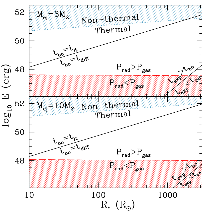
Figure 1.— Main physical conditions that determine shock breakout as a function of $R_{*}$ and $E$. Top and bottom panels are ejecta masses of $3\,M_{\odot}$ and $10\,M_{\odot}$, respectively. The solid line divides regions where the duration $t_{\rm bo}$ is determined by either the light-crossing time $t_{\rm lt}$ or the thermal diffusion time $t_{\rm diff}$. Above the dotted line is the non-thermal regime (blue, lightly shaded). Below the dashed line the shock becomes gas-pressure dominated (red, darkly shaded). In the far right bottom corner, $t_{\rm exp}<t_{\rm bo}$ and the breakout is suppressed by adiabatic expansion.

In Figure 2, I show how these different physical conditions translate into observed luminosities and durations. Solid lines denote constant breakout luminosity, which is set as

$$L_{\rm bo}=\min(E_{\rm rad},E_{\rm gas})/\max(t_{\rm lt},t_{\rm diff}),$$ (11)

where I add an interpolation in each of the $\min$ and $\max$ functions to smooth the transitions. Furthermore, I include a factor of $[1+(t_{\rm bo}/t_{\rm exp})^{3}]^{-\gamma}$ to account for adiabatic expansion (Piro et al., 2010), where $\gamma$ is the adiabatic exponent. The solid lines are labeled by the $x$, where $L_{\rm bo}=10^{x}\,{\rm erg\,s^{-1}}$. The breakout luminosity decreases rapidly once gas pressure dominates, and I shade regions where $L_{\rm bo}<10^{39}\,{\rm erg\,s^{-1}}$. Dotted lines donate constant breakout durations $t_{\rm bo}=\max(t_{\rm lt},t_{\rm diff})$. Red crosses compare core-collapse of a blue supergiant (Ensman & Burrows, 1992) with BH formation from a red supergiant, demonstrating the different regimes these two cases occupy.

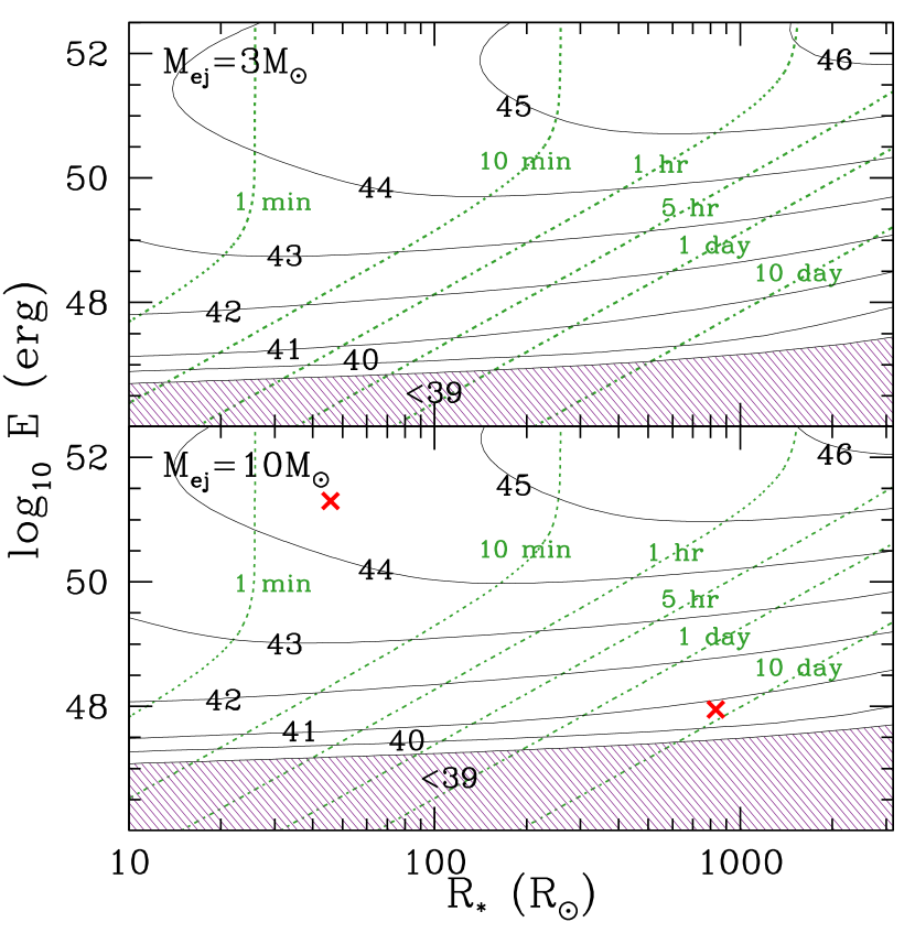
Figure 2.— Same as Figure 1, this time plotting contours of constant breakout luminosity $L_{\rm bo}$ (solid lines) and constant duration $t_{\rm bo}$ (green, dotted lines). The contours are labeled with their values, with the contours of constant luminosity labeled by $x$ where $L_{\rm bo}=10^{x}\,{\rm erg\,s^{-1}}$. Purple, shaded regions denote where $L_{\rm bo}<10^{39}\,{\rm erg\,s^{-1}}$. The decrease in $L_{\rm bo}$ at especially large $R_{*}$ and $E$ (the upper-left and lower-right corners) is due to adiabatic expansion. The upper red cross shows a characteristic model from Ensman & Burrows (1992), which is appropriate for core-collapse of a blue supergiant. The lower red cross corresponds to BH formation of a $15\,M_{\odot}$ ZAMS red supergiant (Lovegrove & Woosley, 2013, maximum mass loss model).

Since it may be generally useful, a wider range of $R_{*}$ and $E$ are plotted in Figures 1 and 2 than just what applies to the BH formation case that is the focus here. For example, for a pair instability SN with $R_{*}\sim 2000\,R_{\odot}$ and $E\sim 10^{52}-10^{53}\,{\rm erg}$, the expectation from Figure 2 is that $L_{\rm bo}\sim 10^{46}\,{\rm erg\,s^{-1}}$ with $t_{\rm bo}\sim{\rm hrs}$. This is roughly consistent with more detailed calculations (Kasen et al., 2011). Similarly, if the luminosity and duration of a purported breakout flash is observed, these results can be used to infer $R_{*}$ and $E$, potentially even providing constraints on transient events that are difficult to classify.

Especially relevant to the situation of BH formation is the regime where $E_{\rm bo}\approx E_{\rm rad}$ and $t_{\rm bo}\approx t_{\rm diff}$, which results in

$$L_{\rm bo}=1.4\times 10^{41}\frac{E_{48}^{1.36}}{\kappa_{0.34}^{0.29}M_{10}^{0.65}R_{1000}^{0.42}}\left(\frac{\rho_{1}}{\rho_{*}}\right)^{0.194}{\rm erg\,s^{-1}}.$$ (12)

This applies to the entire lower-right triangle of parameter space in each of the panels of Figure 1 (although note that adiabatic expansion can cause the luminosity to be somewhat lower than this). The observed shock breakout temperature is in the thermal regime and thus can be estimated as $T_{\rm obs}\approx T_{\rm bo}/\tau_{\rm bo}^{1/4}$, where $T_{\rm bo}$ is the temperature of the plasma at the depth of the breakout, resulting in

$$T_{\rm obs}=1.4\times 10^{4}\frac{E_{48}^{0.34}}{\kappa_{0.34}^{0.068}M_{10}^{0.16}R_{1000}^{0.61}}\left(\frac{\rho_{1}}{\rho_{*}}\right)^{0.049}{\rm K}.$$ (13)

Since $T_{\rm bo}\gtrsim T_{\rm obs}$, an electron scattering opacity is sufficient to estimate the diffusion properties. At the surface, where the temperature is close to $T_{\rm obs}$, other opacity effects may impact the observed spectra, which should be modeled in the future.

Subsequent to the breakout emission, there is a plateau-like phase due to hydrogen recombination as investigated by Lovegrove & Woosley (2013). Using the analytic fits to the numerical models of Type II-P SNe by Kasen & Woosley (2009), I estimate that this phase has a luminosity

$$L_{\rm plat}\approx 2\times 10^{39}\frac{E_{48}^{5/6}R_{1000}^{2/3}}{M_{10}^{1/2}}\,{\rm erg\,s^{-1}},$$ (14)

with a duration of

$$t_{\rm plat}\approx 420\frac{M_{10}^{1/2}R_{1000}^{1/6}}{E_{48}^{1/4}}\,{\rm days},$$ (15)

which roughly matches Lovegrove & Woosley (2013). Comparison between $L_{\rm bo}$ and $L_{\rm plat}$ shows that breakout emission will be more conducive to detection by surveys.

An important constraint on observing the breakout from BH formation is that the shock must have sufficient energy to produce an observable signal. Estimating the breakout duration in the gas-dominated regime,

$$t_{\rm bo}=t_{\rm diff}=7.8\frac{M_{10}^{0.20}R_{1000}^{2.19}}{\kappa_{0.34}^{0.62}E_{48}^{0.81}}\left(\frac{\rho_{1}}{\rho_{*}}\right)^{-0.25}{\rm days},$$ (16)

and the corresponding breakout luminosity is

$$L_{\rm bo}=2.5\times 10^{42}\frac{E_{48}^{5.22}}{\kappa_{0.34}^{1.12}M_{10}^{3.79}R_{1000}^{0.82}}\left(\frac{\rho_{1}}{\rho_{*}}\right)^{-0.95}{\rm erg\,s^{-1}}.$$ (17)

Setting this as $>10^{39}\,{\rm erg\,s^{-1}}$, the shock energy must obey

$$E>2.2\times 10^{47}\kappa_{0.34}^{0.21}M_{10}^{0.73}R_{1000}^{0.16}\left(\frac{\rho_{1}}{\rho_{*}}\right)^{0.18}{\rm erg}.$$ (18)

Lovegrove & Woosley (2013) find values around this range, both above and below, and with generally more energy for a $15\,M_{\odot}$ ZAMS star in comparison to $25\,M_{\odot}$. This suggests that the breakout may not be detectable in all cases. An important focus for future simulations of collapsing stars is to better explore the full range of shock energies possible.

3. Conclusions and Discussion

I have investigated shock breakout during the collapse of a red supergiant producing a BH. The shock is generated by the hydrodynamic response of $\sim{\rm few}\times 0.1M_{\odot}$ being carried away by neutrinos in the time before BH formation. This breakout flash has many distinctive characteristics that will help distinguish it from other potential short timescale transients (e.g., Metzger et al., 2009a, b; Darbha et al., 2010; Metzger et al., 2010; Shen et al., 2010), which I summarize as follows.

1. The breakout flash has a luminosity $L_{\rm bo}\approx 10^{40}-10^{41}{\rm erg\,s^{-1}}$, as given by equation (12).

2. The flash duration is $t_{\rm bo}\approx 3-10\,{\rm days}$ with $t_{\rm bo}\propto R_{*}^{2.16}$ because it is set by $t_{\rm diff}$ (rather than $t_{\rm lc}$ as in many SNe).

3. The breakout is in the thermal regime with an observed temperature of $T_{\rm obs}\approx 10,000\,{\rm K}$.

4. The velocities should be relatively low with $v_{\rm max}\approx 200\,{\rm km\,s^{-1}}$, as given by equation (9).

5. The star likely retained most of its hydrogen envelope to have a sufficiently large radius for a bright and long lasting breakout, and this would be seen in the spectra.

6. The spectrum should be devoid of nucleosynthetic products from explosive burning.

The source would peak in the ultraviolet with an absolute magnitude of roughly $-14.5$. The spectrum will be bright in blue and visual wavebands, making it well-suited for detection by wide-field, transient surveys like the Palomar Transient Factory (PTF; Rau et al., 2009; Law et al., 2009) and the Panoramic Survey Telescope and Rapid Response System (Pan-STARRS; Kaiser et al., 2002). Future theoretical work should better quantify the time-dependent temperature and luminosity during this phase. If the progenitor is a blue supergiant or a Wolf-Rayet star rather than a red supergiant, then the smaller radius causes the shock breakout duration to be significantly shorter than what I summarize here. Nevertheless, the main properties can be estimated using Figure 2.

A critical issue I have explored, which typically does not occur for normal shock breakouts from SNe, is the impact of gas pressure and adiabatic expansion at low shock energies. It is shown that if the shock is sufficiently low energy, as quantified by equation (18), then the breakout will not be observable. A critical question for future theoretical studies will therefore be to explore what exactly is the expected range of energies for this shock. This may depend on many factors, including the progenitor mass, neutron star equation of state, treatment of neutrino emission, and duration of neutrino emission from the protoneutron star prior to collapse to a BH. For example, Lovegrove & Woosley (2013) find that a NS equation of state that favors a massive maximum mass ($\approx 2.5\,M_{\odot}$) results in increased neutrino emission and a stronger shock. This shows how the detection and study of the signal described here could assist in addressing other fundamental questions in physics and astrophysics.

References

- Baumgarte et al. (1996) Baumgarte, T. W., Janka, H.-T., Keil, W., Shapiro, S. L., & Teukolsky, S. A. 1996, ApJ, 468, 823
- Beacom et al. (2001) Beacom, J. F., Boyd, R. N., & Mezzacappa, A. 2001, Phys. Rev. D, 63, 073011
- Burrows (1986) Burrows, A. 1986, ApJ, 300, 488
- Burrows (1988) Burrows, A. 1988, ApJ, 334, 891
- Calzavara & Matzner (2004) Calzavara, A. J., & Matzner, C. D. 2004, MNRAS, 351, 694
- Darbha et al. (2010) Darbha, S., Metzger, B. D., Quataert, E., et al. 2010, MNRAS, 409, 846
- Dexter & Kasen (2012) Dexter, J., & Kasen, D. 2012, arXiv:1210.7240
- Eldridge & Tout (2004) Eldridge, J. J., & Tout, C. A. 2004, MNRAS, 353, 87
- Ensman & Burrows (1992) Ensman, L., & Burrows, A. 1992, ApJ, 393, 742
- Fryer (1999) Fryer, C. L. 1999, ApJ, 522, 413
- Gandel’Man & Frank-Kamenetskii (1956) Gandel’Man, G. M., & Frank-Kamenetskii, D. A. 1956, Soviet Physics Doklady, 1, 223
- Heger et al. (2003) Heger, A., Fryer, C. L., Woosley, S. E., Langer, N., & Hartmann, D. H. 2003, ApJ, 591, 288
- Heger et al. (2005) Heger, A., Woosley, S. E., & Spruit, H. C. 2005, ApJ, 626, 350
- Imshennik & Nadezhin (1989) Imshennik, V. S., & Nadezhin, D. K. 1989, Astrophysics and Space Physics Reviews, 8, 1
- Kaiser et al. (2002) Kaiser, N., Aussel, H., Burke, B. E., et al. 2002, Proc. SPIE, 4836, 154
- Kasen & Woosley (2009) Kasen, D., & Woosley, S. E. 2009, ApJ, 703, 2205
- Kasen et al. (2011) Kasen, D., Woosley, S. E., & Heger, A. 2011, ApJ, 734, 102
- Katz et al. (2012) Katz, B., Sapir, N., & Waxman, E. 2012, ApJ, 747, 147
- Kochanek et al. (2008) Kochanek, C. S., Beacom, J. F., Kistler, M. D., et al. 2008, ApJ, 684, 1336
- Law et al. (2009) Law, N. M., Kulkarni, S. R., Dekany, R. G., et al. 2009, PASP, 121, 1395
- Liebendörfer et al. (2004) Liebendörfer, M., Messer, O. E. B., Mezzacappa, A., et al. 2004, ApJS, 150, 263