Dimension Independent Matrix Square using MapReduce (DIMSUM)

Abstract

We compute the singular values of an $m\times n$ sparse matrix $A$ in a distributed setting, without communication dependence on $m$, which is useful for very large $m$. In particular, we give a simple nonadaptive sampling scheme where the singular values of $A$ are estimated within relative error with constant probability. Our proven bounds focus on the MapReduce framework, which has become the de facto tool for handling such large matrices that cannot be stored or even streamed through a single machine.

On the way, we give a general method to compute $A^{T}A$. We preserve singular values of $A^{T}A$ with $\epsilon$ relative error with shuffle size $O(n^{2}/\epsilon^{2})$ and reduce-key complexity $O(n/\epsilon^{2})$. We further show that if only specific entries of $A^{T}A$ are required and $A$ has nonnegative entries, then we can reduce the shuffle size to $O(n\log(n)/s)$ and reduce-key complexity to $O(\log(n)/s)$, where $s$ is the minimum cosine similarity for the entries being estimated. All of our bounds are independent of $m$, the larger dimension. We provide open-source implementations in Spark and Scalding, along with experiments in an industrial setting.

1 Introduction

There has been a flurry of work to solve problems in numerical linear algebra via fast approximate randomized algorithms. Starting with [19] many algorithms have been proposed over older algorithms [13, 14, 15, 11, 16, 17, 12, 18, 8, 26, 5, 6, 22], with results satisfying the traditional Monte Carlo performance guarantees: small error with high probability.

These proposed algorithms require either streaming, or having access to the entire matrix $A$ on a single machine, or communicating too much data between machines. This is not feasible for very large $m$ (for example $m=10^{13}$). In such cases, $A$ cannot be stored or streamed through a single machine - let alone be used in computations. For such cases, MapReduce [9] has become the de facto tool for handling very large datasets.

MapReduce is a programming model for processing large data sets, typically used to do distributed computing on clusters of commodity computers. With large amount of processing power at hand, it is very tempting to solve problems by brute force. However, we combine clever sampling techniques with the power of MapReduce to extend its utility.

Given an $m\times n$ matrix $A$ with each row having at most $L$ nonzero entries, we show how to compute the singular values and and right singular vectors of $A$ without dependence on $m$, in a MapReduce environment. The SVD of $A$ is written $A=U\Sigma V^{T}$, where $U$ is $m\times n$, $\Sigma$ is $n\times n$, and $V$ is $n\times n$.

We compute $\Sigma$ and $V$. We do this by first computing $A^{T}A$, which we do without dependence on $m$. Since $A^{T}A=V\Sigma^{2}V^{T}$ is $n\times n$, for small $n$ (for example $n=10^{4}$) we can compute the eigen-decomposition of $A^{T}A$ directly and retrieve $V$ and $\Sigma$. What remains is to compute $A^{T}A$ efficiently and without harming its singular values, which is what the rest of the paper is focused on.

Our main result is Algorithms 3 and 4, along with proven guarantees given in Theorem Theorem which proves a relative error bound using the spectral norm. The proof uses a new singular value concentration inequality from [23] that has not seen much usage by the theoretical computer science community.

2 Formal Preliminaries

Label the columns of $A$ as $c_{1},\ldots,c_{n}$, rows as $r_{1},\ldots,r_{m}$, and the individual entries as $a_{ij}$. The matrix is stored row-by-row on disk and read via mappers. We focus on the case where each dimension is sparse with at most $L$ nonzeros per row therefore the natural way to store the data is to segment into rows. Throughout the paper we assume the entries of $A$ have been scaled to be in $[-1,1]$, which can be done with little communication by finding the largest magnitude element.

We use the matrix spectral norm throughout, which for any $m\times n$ matrix $A$ is defined as

$$||A||_{2}=\max_{x\in\mathbb{R}^{m},y\in\mathbb{R}^{n}}\frac{x^{T}Ay}{||x||_{2}||y||_{2}}$$

Unless otherwise denoted, the norm used anywhere in this paper is the spectral norm, which for regular vectors degenerates to the vector $l_{2}$ norm.

We concentrate on the regime where $m$ is very large, e.g. $m=10^{13}$, but $n$ is not too large, e.g. $n=10^{4}$, such that we can compute the SVD of an $n\times n$ dense matrix on a single machine. The magnitudes of each column is assumed to be loaded into memory and available to both the mappers and reducers. The magnitudes of each column are natural values to have computed already, or can be computed with a trivial mapreduce.

2.1 Naive Computation

The naive way to compute $A^{T}A$ on MapReduce is to materialize all dot products between columns of $A$ trivially. For purposes of demonstrating the complexity measures for MapReduce, we briefly write down the Naive algorithm to compute $A^{T}A$.

Algorithm 1 NaiveMapper$(r_{i})$

  for all pairs $(a_{ij},a_{ik})$ in $r_{i}$ do

        Emit $((c_{j},c_{k})\rightarrow a_{ij}a_{ik})$

  end for

Algorithm 2 NaiveReducer$((c_{i},c_{j}),\langle v_{1},\ldots,v_{R}\rangle)$

  output $c_{i}^{T}c_{j}\rightarrow\sum_{i=1}^{R}v_{i}$

2.2 Complexity Measures

There are two main complexity measures for MapReduce: “shuffle size”, and “reduce-key complexity”. These complexity measures together capture the bottlenecks when handling data on multiple machines: first we can’t have too much communication between machines, and second we can’t overload a single machine. The number of emissions in the map phase is called the “shuffle size”, since that data needs to be shuffled around the network to reach the correct reducer. The maximum number of items reduced to a single key is called the “reduce-key complexity” and measures how overloaded a single machine may become [20].

It can be easily seen that the naive approach for computing $A^{T}A$ will have $O(mL^{2})$ emissions, which for the example parameters we gave ($m=10^{13},n=10^{4},L=20)$ is infeasible. Furthermore, the maximum number of items reduced to a single key can be as large as $m$. Thus the “reduce-key complexity” for the naive scheme is $m$.

We can drastically reduce the shuffle size and reduce-key complexity by some clever sampling with the DIMSUM scheme described in this paper. In this case, the output of the reducers are random variables whose expectations are cosine similarities i.e. normalized entries of $A^{T}A$. Two proofs are needed to justify the effectiveness of this scheme. First, that the expectations are indeed correct and obtained with constant probability, and second, that the shuffle size is greatly reduced. We prove both of these claims. In particular, in addition to correctness, we prove that for relative error $\epsilon$, the shuffle size of our scheme is only $O(n^{2}/\epsilon^{2})$, with no dependence on the dimension $m$, hence the title of this paper.

This means as long as there are enough mappers to read the data, our sampling scheme can be used to make the shuffle size tractable. Furthermore, each reduce-key gets at most $O(n/\epsilon^{2})$ values, thus making the reduce-key complexity tractable, too. Within Twitter Inc, we use the DIMSUM sampling scheme to compute similar users [28, 21]. We have also used the scheme to find highly similar pairs of words, by taking each dimension to be the indicator vector that signals in which tweets the word appears. We empirically verified the proven claims in this paper, but do not report experimental results since we are primarily focused on the proofs.

2.3 Related Work

[19] introduced a sampling procedure where rows and columns of $A$ are picked with probabilities proportional to their squared lengths and used that to compute an approximation to $A^{T}A$. Later [1] and [2] improved the sampling procedure. To implement these approximations to $A^{T}A$ on MapReduce one would need a shuffle size dependent on $m$ or overload a single machine. We improve this to be independent of $m$ both in shuffle size and reduce-key complexity.

Later on [10] found an adaptive sampling scheme to improve the scheme of [19]. Since the scheme is adaptive, it would require too much communication between machines holding $A$. In particular a MapReduce implementation would still have shuffle size dependent on $m$, and require many (more than 1) iterations.

There has been some effort to reduce the number of passes required through the matrix $A$ using little memory, in the streaming model [7]. The question was posed by [24] to determine in the streaming model various linear algebraic quantities. The problem was posed again by [25] who asked about the time and space required for an algorithm not using too many passes. The streaming model is a good one if all the data can be streamed through a single machine, but with $m$ so large, it is not possible to stream $A$ through a single machine. Splitting the work of reading $A$ across many mappers is the job of the MapReduce implementation and one of its major advantages [9].

There has been recent work specifically targeted at computing the SVD on MapReduce [3] in a stable manner via $QR$ factorizations and bypassing $A^{T}A$, with shuffle size and reduce-key complexity both dependent on $m$.

In addition to computing entries of $A^{T}A$, our sampling scheme can be used to implement many similarity measures. We can use the scheme to efficiently compute four similarity measures: Cosine, Dice, Overlap, and the Jaccard similarity measures, with details and experiments given in [27, 21], whereas this paper is more focused on matrix computations and an open-source implementation.

3 Algorithm

Our algorithm to compute $A^{T}A$ efficiently is given below in Algorithms 3 and 4.

Algorithm 3 DIMSUMMapper$(r_{i})$

  for all pairs $(a_{ij},a_{ik})$ in $r_{i}$ do

        With probability

$$\min\left(1,\gamma\frac{1}{||c_{j}||||c_{k}||}\right)$$

emit $((c_{j},c_{k})\rightarrow a_{ij}a_{ik})$

  end for

Algorithm 4 DIMSUMReducer$((c_{i},c_{j}),\langle v_{1},\ldots,v_{R}\rangle)$

  if $\frac{\gamma}{||c_{i}||||c_{j}||}>1$ then

        output $b_{ij}\rightarrow\frac{1}{||c_{i}||||c_{j}||}\sum_{i=1}^{R}v_{i}$

  else

        output $b_{ij}\rightarrow\frac{1}{\gamma}\sum_{i=1}^{R}v_{i}$

  end if

It is important to observe what happens if the output ‘probability’ is greater than 1. We certainly Emit, but when the output probability is greater than 1, care must be taken while reducing to scale by the correct factor, since it won’t be correct to divide by $\gamma$, which is the usual case when the output probability is less than 1. Instead, the sum in Algorithm 4 obtains the dot product, because for the pairs where the output probability is greater than 1, DIMSUMMapper effectively always emits. We do not repeat this point later in the paper, nonetheless it is an important one which arises during implementation.

4 Correctness

Before we move onto the correctness of the algorithm, we must state Latala’s Theorem [23]. This theorem talks about a general model of random matrices whose entries are independent centered random variables with some general distribution (not necessarily normal). The largest singular value (the spectral norm) can be estimated by Latala’s theorem for general random matrices with non-identically distributed entries:

Theorem.

[23]. Let $X$ be a random matrix whose entries $x_{ij}$ are independent centered random variables with finite fourth moment. Denoting $||X||_{2}$ as the matrix spectral norm, we have

$$\operatorname*{\mathbb{E}}||X||_{2}\leq C\left[\max_{i}\left(\sum_{j}\operatorname*{\mathbb{E}}x_{ij}^{2}\right)^{1/2}+\max_{j}\left(\sum_{i}\operatorname*{\mathbb{E}}x_{ij}^{2}\right)^{1/2}+\left(\sum_{i,j}\operatorname*{\mathbb{E}}x_{ij}^{4}\right)^{1/4}\right].$$

We analyze the second and fourth central moments of the entries of the estimate for $A^{T}A$, and show that by Latala’s theorem, the singular values are preserved with constant probability. Let the matrix output by the DIMSUM algorithm be called $B$ with entries $b_{ij}$. Notice that this is an $n\times n$ matrix of cosine similarities between columns of $A$. Define a diagonal matrix $D$ with $d_{ii}=||c_{i}||$. Then we can undo the cosine similarity normalization to obtain an estimate for $A^{T}A$ by using $DBD$. This effectively uses the cosine similarities between columns of $A$ as an importance sampling scheme. We have the following theorem:

Theorem.

Let $A$ be an $m\times n$ matrix with $m>n$. If $\gamma=\Omega(n/\epsilon^{2})$ and $D$ a diagonal matrix with entries $d_{ii}=||c_{i}||$, then the matrix $B$ output by DIMSUM (Algorithms 3 and 4) satisfies,

$$\frac{||DBD-A^{T}A||_{2}}{||A^{T}A||_{2}}\leq\epsilon$$

with probability at least $1/2$.

Proof.

We define the indicator variable $X_{ijk}$ to take value $a_{ki}a_{kj}$ with probability $p_{ij}=\gamma\frac{1}{||c_{i}||||c_{j}||}$ on the $k$’th call to DIMSUMMapper, and zero with probability $1-p_{ij}$.

$$X_{ijk}=\left\{\begin{array}[]{ll}a_{kj}a_{kj}&\mbox{with prob. }p_{ij}\\ 0&\mbox{with prob. }1-p_{ij}\end{array}\right.$$

Then we can write the entries of $B$ as

$$b_{ij}=\frac{1}{\gamma}\sum_{k=1}^{m}X_{ijk}$$

Since we give relative error bounds and singular values scale trivially, we can assume $A$ has all entries in $[0,1]$. i.e. any scaling of the input matrix will have the same relative error guarantee. This assumption will be useful because we first prove an absolute error bound, then use that to prove a relative error bound. It should be clear from the definitions that in expectation

$$E[B]=D^{-1}A^{T}AD^{-1}\text{ and }E[DBD]=A^{T}A$$

With these definitions, we now move onto bounding $\operatorname*{\mathbb{E}}[||B-D^{-1}A^{T}AD^{-1}||]$. With the goal of invoking Latala’s theorem, we analyze $\operatorname*{\mathbb{E}}[(b_{ij}-Eb_{ij})^{2}]$ and $\operatorname*{\mathbb{E}}[(b_{ij}-Eb_{ij})^{4}]$.

Now define $\#(i,j)$ as the number of dimensions in which $c_{i}$ and $c_{j}$ are both nonzero, i.e. the number of $k$ for which $a_{ki}a_{kj}$ is nonzero, and further define $i\cap j$ as the set of indices for which $a_{ki}a_{kj}$ is nonzero.

Clearly, $\operatorname*{\mathbb{E}}[(b_{ij}-Eb_{ij})^{2}]$ is the variance of $b_{ij}$, which is the sum of $\#(i,j)$ weighted indicator random variables. Thus we have

$$\operatorname*{\mathbb{E}}[(b_{ij}-Eb_{ij})^{2}]=\text{Var}[b_{ij}]=\frac{1}{\gamma^{2}}\sum_{k\in i\cap j}\text{Var}[X_{ijk}]$$

$$=\frac{1}{\gamma^{2}}\sum_{k\in i\cap j}a_{ki}^{2}a_{kj}^{2}p_{ij}(1-p_{ij})$$

$$\leq\frac{1}{\gamma^{2}}\sum_{k\in i\cap j}a_{ki}^{2}a_{kj}^{2}p_{ij}$$

$$=\frac{1}{\gamma^{2}}\sum_{k\in i\cap j}a_{ki}^{2}a_{kj}^{2}\gamma\frac{1}{||c_{i}||||c_{j}||}$$

Now by the Arithmetic-Mean Geometric-Mean inequality,

$$\leq\frac{1}{2\gamma^{2}}\sum_{k\in i\cap j}a_{ki}^{2}a_{kj}^{2}\gamma\left(\frac{1}{||c_{i}||^{2}}+\frac{1}{||c_{j}||^{2}}\right)$$

$$=\frac{1}{2\gamma}\sum_{k\in i\cap j}a_{ki}^{2}a_{kj}^{2}\left(\frac{1}{||c_{i}||^{2}}+\frac{1}{||c_{j}||^{2}}\right)$$

$$\leq\frac{1}{\gamma}\sum_{k\in i\cap j}a_{ki}^{2}a_{kj}^{2}\left(\frac{1}{||c_{j}||^{2}}\right)$$

$$\leq\frac{1}{\gamma}\sum_{k\in i\cap j}\frac{a_{kj}^{2}}{||c_{j}||^{2}}\leq\frac{1}{\gamma}$$

Thus we have $E[(b_{ij}-Eb_{ij})^{2}]\leq\frac{1}{\gamma}$. It remains to bound the fourth central moment of $b_{ij}$. We use a counting trick to achieve this bound:

$$\operatorname*{\mathbb{E}}[(b_{ij}-Eb_{ij})^{4}]=\frac{1}{\gamma^{4}}\operatorname*{\mathbb{E}}\left[\left(\sum_{k\in i\cap j}X_{ijk}-a_{ki}a_{kj}p_{ij}\right)^{4}\right]$$

$$=\frac{1}{\gamma^{4}}\operatorname*{\mathbb{E}}\left[\sum_{q,r,s,t\in i\cap j}(X_{ijq}-a_{qi}a_{qj}p_{ij})(X_{ijr}-a_{ri}a_{rj}p_{ij})(X_{ijs}-a_{si}a_{sj}p_{ij})(X_{ijt}-a_{ti}a_{tj}p_{ij})\right]$$

$$=\frac{1}{\gamma^{4}}\sum_{q,r,s,t\in i\cap j}\operatorname*{\mathbb{E}}\left[(X_{ijq}-a_{qi}a_{qj}p_{ij})(X_{ijr}-a_{ri}a_{rj}p_{ij})(X_{ijs}-a_{si}a_{sj}p_{ij})(X_{ijt}-a_{ti}a_{tj}p_{ij})\right]$$

which effectively turns this into a counting problem. The terms in the sum on the last expression are 0 unless either $q=r=s=t$, which happens $\#(i,j)$ times, or there are two pairs of matching indices, which happens ${\#(i,j)\choose 2}{4\choose 2}$ times. Continuing, this gives us

$$=\frac{1}{\gamma^{4}}\sum_{k\in i\cap j}\operatorname*{\mathbb{E}}[(X_{ijk}-a_{ki}a_{kj}p_{ij})^{4}]+\frac{1}{\gamma^{4}}\sum_{q,r\in i\cap j}\text{Var}[X_{ijq}]\text{Var}[X_{ijr}]$$

$$=\frac{1}{\gamma^{4}}\sum_{k\in i\cap j}a_{ki}^{4}a_{kj}^{4}[p_{ij}^{4}(1-p_{ij})+(1-p_{ij})^{4}p_{ij}]$$

$$+\frac{1}{\gamma^{4}}\sum_{q,r\in i\cap j}a_{qi}^{2}a_{qj}^{2}p_{ij}(1-p_{ij})a_{ri}^{2}a_{rj}^{2}p_{ij}(1-p_{ij})$$

$$\leq\frac{1}{\gamma^{4}}\sum_{k\in i\cap j}a_{ki}^{4}a_{kj}^{4}p_{ij}+\frac{1}{\gamma^{4}}\sum_{q,r\in i\cap j}a_{qi}^{2}a_{qj}^{2}a_{ri}^{2}a_{rj}^{2}p_{ij}^{2}$$

$$=\frac{1}{\gamma^{3}}\frac{1}{||c_{i}||||c_{j}||}\sum_{k\in i\cap j}a_{ki}^{4}a_{kj}^{4}+\frac{1}{\gamma^{2}}\frac{1}{||c_{i}||^{2}||c_{j}||^{2}}\sum_{q,r\in i\cap j}a_{qi}^{2}a_{qj}^{2}a_{ri}^{2}a_{rj}^{2}$$

by the Arithmetic-Mean Geometric-Mean inequality,

$$\leq\frac{1}{2\gamma^{3}}(\frac{1}{||c_{i}||^{2}}+\frac{1}{||c_{j}||^{2}})\sum_{k\in i\cap j}a_{ki}^{4}a_{kj}^{4}+\frac{1}{\gamma^{2}}\frac{1}{||c_{i}||^{2}||c_{j}||^{2}}\sum_{q,r\in i\cap j}a_{qi}^{2}a_{qj}^{2}a_{ri}^{2}a_{rj}^{2}$$

and since entries $a_{ij}\in[0,1]$,

$$\leq\frac{1}{2\gamma^{3}}(\frac{1}{||c_{i}||^{2}}+\frac{1}{||c_{j}||^{2}})\sum_{k\in i\cap j}a_{ki}^{2}a_{kj}^{2}+\frac{1}{\gamma^{2}}\frac{1}{||c_{i}||^{2}||c_{j}||^{2}}\sum_{q,r\in i\cap j}a_{qi}^{2}a_{rj}^{2}$$

$$\leq\frac{1}{\gamma^{3}}\frac{1}{||c_{i}||^{2}}\sum_{k\in i\cap j}a_{ki}^{2}+\frac{1}{\gamma^{2}}\frac{1}{||c_{i}||^{2}||c_{j}||^{2}}\sum_{q,r\in i\cap j}a_{qi}^{2}a_{rj}^{2}$$

$$\leq\frac{1}{\gamma^{3}}+\frac{1}{\gamma^{2}}$$

for $\gamma\geq 1$,

$$\leq\frac{2}{\gamma^{2}}$$

Thus we have that $\operatorname*{\mathbb{E}}[(b_{ij}-Eb_{ij})^{4}]\leq\frac{2}{\gamma^{2}}$, and from the above we have $\operatorname*{\mathbb{E}}[(b_{ij}-Eb_{ij})^{2}]\leq\frac{1}{\gamma}$. Plugging these into Theorem Theorem, we can bound the absolute error between $B$ and $D^{-1}A^{T}AD^{-1}$,

$$\operatorname*{\mathbb{E}}[||B-D^{-1}A^{T}AD^{-1}||]\leq C_{0}[\max_{i}\left(\sum_{j}\operatorname*{\mathbb{E}}[(b_{ij}-Eb_{ij})^{2}]\right)^{1/2}$$

$$+\max_{j}\left(\sum_{i}\operatorname*{\mathbb{E}}[(b_{ij}-Eb_{ij})^{2}]\right)^{1/2}+\left(\sum_{i,j}\operatorname*{\mathbb{E}}[(b_{ij}-Eb_{ij})^{4}]\right)^{1/4}]$$

$$\leq C_{0}[\left(\frac{n}{\gamma}\right)^{1/2}+\left(\frac{n}{\gamma}\right)^{1/2}+\left(\frac{2n^{2}}{\gamma^{2}}\right)^{1/4}]$$

$$\leq C_{1}\left(\frac{n}{\gamma}\right)^{1/2}$$

where $C_{0}$ and $C_{1}$ are absolute constants. Thus we have that

$$\operatorname*{\mathbb{E}}[||B-D^{-1}A^{T}AD^{-1}||]\leq C_{1}\left(\frac{n}{\gamma}\right)^{1/2}$$

Setting $\gamma=4C_{1}^{2}\frac{n}{\epsilon^{2}}$, gives

$$E[||B-D^{-1}A^{T}AD^{-1}||]\leq\epsilon/2$$

Thus by the Markov inequality we have with probability at least $1/2$,

$$||B-D^{-1}A^{T}AD^{-1}||\leq\epsilon$$

Which gives us an absolute error bound between $B$ and $D^{-1}A^{T}AD^{-1}$. It remains to get a relative error bound between $DBD$ and $A^{T}A$,

$$\frac{||DBD-A^{T}A||}{||A^{T}A||}=\frac{||D(B-D^{-1}A^{T}AD^{-1})D||}{||A^{T}A||}$$

by the submultiplicative property of the spectral norm,

$$\leq\frac{||D||^{2}||B-D^{-1}A^{T}AD^{-1}||}{||A^{T}A||}$$

Now since $D$ is a diagonal matrix with positive entries, its spectral norm is its largest entry, i.e. the largest column magnitude, call it $c_{*}$,

$$\leq\frac{c_{*}^{2}||B-D^{-1}A^{T}AD^{-1}||}{||A^{T}A||}$$

Now we use another property of the spectral norm to lowerbound $||A^{T}A||$,

$$||A^{T}A||=\max_{x,y\in\mathbb{R}^{n}}\frac{x^{T}A^{T}Ay}{||x||||y||}$$

Setting $x,y$ to be indicator vectors to pick out the $i$’th diagonal entry of $A^{T}A$, we have that $||A^{T}A||\geq c_{*}^{2}$ since $c_{*}^{2}$ is some entry in the diagonal of $A^{T}A$. In addition to allowing us to bound the fourth central moment, this is yet another reason why we picked the sampling probabilities in Algorithm 3. Finally, continuing from above armed with this lower bound,

$$\frac{||DBD-A^{T}A||}{||A^{T}A||}\leq\frac{c_{*}^{2}||B-D^{-1}A^{T}AD^{-1}||}{||A^{T}A||}$$

$$\leq\frac{c_{*}^{2}\epsilon}{||A^{T}A||}$$

$$\leq\frac{c_{*}^{2}\epsilon}{c_{*}^{2}}$$

$$=\epsilon$$

with probability at least $1/2$.

∎

Although we had to set $\gamma=\Omega(n/\epsilon^{2})$ to estimate the singular values, if instead of the singular values we are interested in individual entries of $A^{T}A$ that are large, we can get away setting $\gamma$ significantly smaller, and thus reducing shuffle size. In particular if two columns have high cosine similarity, we can estimate the corresponding entry in $A^{T}A$ with much less computation. Here we define cosine similarity as the normalized dot product

$$\cos(c_{i},c_{j})=\frac{c_{i}^{T}c_{j}}{||c_{i}||||c_{j}||}$$

Theorem.

Let $A$ be an $m\times n$ matrix with entries in $[0,1]$. For any two columns $c_{i}$ and $c_{j}$ having $\cos(c_{i},c_{j})\geq\epsilon$, let $B$ be the output of DIMSUM with entries $b_{ij}=\frac{1}{\gamma}\sum_{k=1}^{m}X_{ijk}$ with $X_{ijk}$ as defined in Theorem Theorem. Now if $\gamma\geq\alpha/\epsilon$, then we have,

$$\Pr\left[||c_{i}||||c_{j}||b_{ij}>(1+\delta)[A^{T}A]_{ij}\right]\leq\left(\frac{e^{\delta}}{(1+\delta)^{(1+\delta)}}\right)^{\alpha}$$

and

$$\Pr\left[||c_{i}||||c_{j}||b_{i,j}<(1-\delta)[A^{T}A]_{ij}\right]<\exp(-\alpha\delta^{2}/2)$$

Proof.

We use $||c_{i}||||c_{j}||b_{i,j}$ as the estimator for $[A^{T}A]_{ij}$. Note that

$$\mu_{ij}=\operatorname*{\mathbb{E}}[\sum_{k=1}^{m}X_{ijk}]=\gamma\frac{c_{i}^{T}c_{j}}{||c_{i}||||c_{j}||}=\gamma\cos(x,y)\geq\alpha$$

Thus by the multiplicative form of the Chernoff bound,

$$\Pr\left[||c_{i}||||c_{j}||b_{ij}>(1+\delta)[A^{T}A]_{ij}\right]=\Pr\left[\gamma\frac{||c_{i}||||c_{j}||}{||c_{i}||||c_{j}||}b_{ij}>\gamma(1+\delta)\frac{[A^{T}A]_{ij}}{||c_{i}||||c_{j}||}\right]$$

$$=\Pr\left[\sum_{k=1}^{m}X_{ijk}>(1+\delta)\operatorname*{\mathbb{E}}[\sum_{k=1}^{m}X_{ijk}]\right]\leq\left(\frac{e^{\delta}}{(1+\delta)^{(1+\delta)}}\right)^{\alpha}$$

Similarly, by the other side of the multiplicative Chernoff bound, we have

$$\Pr\left[||c_{i}||||c_{j}||b_{ij}<(1+\delta)[A^{T}A]_{ij}\right]=\Pr\left[\gamma\frac{||c_{i}||||c_{j}||}{||c_{i}||||c_{j}||}b_{ij}<\gamma(1+\delta)\frac{[A^{T}A]_{ij}}{||c_{i}||||c_{j}||}\right]$$

$$=\Pr\left[\sum_{k=1}^{m}X_{ijk}<(1+\delta)\operatorname*{\mathbb{E}}[\sum_{k=1}^{m}X_{ijk}]\right]$$

$$<\exp(-\mu_{ij}\delta^{2}/2)\leq\exp(-\alpha\delta^{2}/2)$$

∎

5 Shuffle Size

Define $H$ as the smallest nonzero entry of $A$ in magnitude, after the entries of $A$ have been scaled to be in $[0,1]$. For example when $A$ has entries in $\{0,1\}$, we have $H=1$.

Theorem.

Let $A$ be an $m\times n$ sparse matrix with at most $L$ nonzeros per row. The expected shuffle size for DIMSUMMapper is $O(nL\gamma/H^{2})$.

Proof.

Define $\#(c_{i},c_{j})$ as the number of dimensions in which $c_{i}$ and $c_{j}$ are both nonzero, i.e. number of $k$ for which $a_{ki}a_{kj}$ is nonzero.

The expected contribution from each pair of columns will constitute the shuffle size:

$$\sum_{i=1}^{n}\sum_{j=i+1}^{n}\sum_{k=1}^{\#(c_{i},c_{j})}\text{Pr}[\text{DIMSUMMapper}(c_{i},c_{j})]$$

$$=\sum_{i=1}^{n}\sum_{j=i+1}^{n}\#(c_{i},c_{j})\text{Pr}[\text{DIMSUMMapper}(c_{i},c_{j})]$$

$$=\sum_{i=1}^{n}\sum_{j=i+1}^{n}\gamma\frac{\#(c_{i},c_{j})}{||c_{i}||||c_{j}||}$$

By the Arithmetic-Mean Geometric-Mean inequality,

$$\leq\frac{\gamma}{2}\sum_{i=1}^{n}\sum_{j=i+1}^{n}\#(c_{i},c_{j})(\frac{1}{||c_{i}||^{2}}+\frac{1}{||c_{j}||^{2}})$$

$$\leq\gamma\sum_{i=1}^{n}\frac{1}{||c_{i}||^{2}}\sum_{j=1}^{n}\#(c_{i},c_{j})$$

$$\leq\gamma\sum_{i=1}^{n}\frac{1}{||c_{i}||^{2}}L||c_{i}||^{2}/H^{2}=\gamma Ln/H^{2}$$

The first inequality holds because of the Arithmetic-Mean Geometric-Mean inequality applied to $\{1/||c_{i}||,1/||c_{j}||\}$. The last inequality holds because $c_{i}$ can co-occur with at most $||c_{i}||^{2}L/H^{2}$ other columns. It is easy to see via Chernoff bounds that the above shuffle size is obtained with high probability.

∎

Theorem.

Let $A$ be an $m\times n$ sparse matrix $A$ with at most $L$ nonzeros per row. The shuffle size for any algorithm computing those entries of $A^{T}A$ for which $\cos(i,j)\geq\epsilon$ is at least $\Omega(nL)$.

Proof.

To see the lowerbound, we construct a dataset consisting of $n/L$ distinct rows of length $L$, furthermore each row is duplicated $L$ times. To construct this dataset, consider grouping the columns into $n/L$ groups, each group containing $L$ columns. A row is associated with every group, consisting of all the columns in the group. This row is then repeated $L$ times. In each group, it is trivial to check that all pairs of columns have cosine similarity exactly 1. There are ${L\choose 2}$ pairs for each group and there are $n/L$ groups, making for a total of $(n/L){L\choose 2}=\Omega(nL)$ pairs with similarity 1, and thus also at least $\epsilon$. Since any algorithm that purports to accurately calculate highly-similar pairs must at least output them, and there are $\Omega(nL)$ such pairs, we have the lower bound. ∎

Theorem.

Let $A$ be an $m\times n$ matrix with non-negative entries. The expected number of values mapped to a single key by DIMSUMMapper is at most $\gamma/H^{2}$.

Proof.

Note that the output of DIMSUMReducer is a number between 0 and 1. Since this is obtained by normalizing the sum of all values reduced to the key by at most $\gamma$, and all summands are at least $H^{2}$, we get that the number of summands is at most $\gamma/H^{2}$. ∎

6 Reducing Computation

In DIMSUMMapper, it is required to generate $L\choose 2$ random numbers for each row, which doesn’t cause communication between machines, but does require computation. We can reduce this computation by moving the random number generation as in Algorithm 5, which uses the summation reducer. However, in Algorithm 5 it is no longer true that the $b_{ij}$ are pairwise independent, and thus an analog of Theorem Theorem does not hold for Algorithm 5. However, Theorem Theorem does hold, as it does not require the $b_{ij}$ to be be pairwise independent, and so when cosine similarities are sought, this is a useful modification.

Algorithm 5 LeanDIMSUMMapper$(r_{i})$

  for all $a_{ij}$ in $r_{i}$ do

        With probability $\min\left(1,\frac{\sqrt{\gamma}}{||c_{j}||}\right)$

        for all $a_{ik}$ in $r_{i}$ do

              With probability $\min\left(1,\frac{\sqrt{\gamma}}{||c_{k}||}\right)$emit $(b_{jk}\rightarrow\frac{a_{ij}a_{ik}}{\min(\sqrt{\gamma},||c_{j}||)\min(\sqrt{\gamma},||c_{k}||)})$

        end for

  end for

7 Experiments and Open Source Code

We run DIMSUM daily on a production-scale ads dataset at Twitter [4]. Upon replacing the traditional cosine similarity computation in late June 2014, we observed 40% improvement in several performance measures, plotted in Figure 1. The y-axis ranges from 0 to hundred of terabytes, where the exact amount is kept confidential.

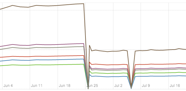
Figure 1: DIMSUM turned on in late June. The y-axis ranges from 0 bytes to hundreds of terabytes.

We have contributed an implementation of DIMSUM to two open source projects: Scalding and Spark [29]. The Spark implementation is widely distributed by many commercial vendors that package Spark with their industrial cluster installations.

• Spark github pull-request: https://github.com/apache/spark/pull/1778

• Scalding github pull-request: https://github.com/twitter/scalding/pull/833

8 Conclusions and Future Directions

We presented the DIMSUM algorithm to compute $A^{T}A$ for an $m\times n$ matrix $A$ with $m>n$. All of our results are provably independent of the dimension $m$, meaning that apart from the initial cost of trivially reading in the data, all subsequent operations are independent of the dimension, the dimension can thus be very large.

Although we used $A^{T}A$ in the context of computing singular values, there are likely other linear algebraic quantities that can benefit from having a provably efficient and accurate MapReduce implementation of $A^{T}A$. For example if one wishes to use the estimate for $A^{T}A$ in solving the normal equations in the ubiquitous least-squares problem

$$A^{T}Ax=A^{T}y$$

then the guarantee given by Theorem Theorem gives some handle on the problem, although a concrete error bound is left for future work.

9 Acknowledgements

We thank the Twitter Personalization and Recommender systems team for allowing us to use production data from the live Twitter site for experiments (not reported), and Kevin Lin for the implementation in the Twitter Ads team. We also thank Jason Lee, Yuekai Sun, and Ernest Ryu from Stanford ICME for valuable discussions. Finally we thank the Stanford student group: Computational Consulting and all its members for their help.

References

- [1] Dimitris Achlioptas and Frank McSherry. Fast computation of low rank matrix approximations. In Proceedings of the thirty-third annual ACM symposium on Theory of computing, pages 611–618. ACM, 2001.
- [2] Sanjeev Arora, Elad Hazan, and Satyen Kale. A fast random sampling algorithm for sparsifying matrices. Approximation, Randomization, and Combinatorial Optimization. Algorithms and Techniques, pages 272–279, 2006.
- [3] Austin R Benson, David F Gleich, and James Demmel. Direct qr factorizations for tall-and-skinny matrices in mapreduce architectures. arXiv preprint arXiv:1301.1071, 2013.
- [4] Reza Bosagh Zadeh. Twitter engineering blog: All-pairs similarity via dimsum. Twitter Engineering Blog, 2014.
- [5] Matthew Brand. Fast low-rank modifications of the thin singular value decomposition. Linear algebra and its applications, 415(1):20–30, 2006.
- [6] Moody T Chu, Robert E Funderlic, and Robert J Plemmons. Structured low rank approximation. Linear algebra and its applications, 366:157–172, 2003.
- [7] Kenneth L Clarkson and David P Woodruff. Numerical linear algebra in the streaming model. In Proceedings of the 41st annual ACM symposium on Theory of computing, pages 205–214. ACM, 2009.
- [8] Kenneth L Clarkson and David P Woodruff. Low rank approximation and regression in input sparsity time. arXiv preprint arXiv:1207.6365, 2012.
- [9] J. Dean and S. Ghemawat. MapReduce: Simplified data processing on large clusters. Communications of the ACM, 51(1):107–113, 2008.
- [10] Amit Deshpande and Santosh Vempala. Adaptive sampling and fast low-rank matrix approximation. Approximation, Randomization, and Combinatorial Optimization. Algorithms and Techniques, pages 292–303, 2006.
- [11] Petros Drineas, Eleni Drinea, and Patrick Huggins. An experimental evaluation of a monte-carlo algorithm for singular value decomposition. Advances in Informatics, pages 279–296, 2003.
- [12] Petros Drineas, Alan Frieze, Ravi Kannan, Santosh Vempala, and V Vinay. Clustering large graphs via the singular value decomposition. Machine learning, 56(1):9–33, 2004.
- [13] Petros Drineas, Ravi Kannan, and Michael W Mahoney. Fast monte carlo algorithms for matrices i: Approximating matrix multiplication. SIAM Journal on Computing, 36(1):132–157, 2006.
- [14] Petros Drineas, Ravi Kannan, and Michael W Mahoney. Fast monte carlo algorithms for matrices ii: Computing a low-rank approximation to a matrix. SIAM Journal on Computing, 36(1):158–183, 2006.
- [15] Petros Drineas, Ravi Kannan, and Michael W Mahoney. Fast monte carlo algorithms for matrices iii: Computing a compressed approximate matrix decomposition. SIAM Journal on Computing, 36(1):184–206, 2006.
- [16] Petros Drineas, Malik Magdon-Ismail, Michael W Mahoney, and David P Woodruff. Fast approximation of matrix coherence and statistical leverage. arXiv preprint arXiv:1109.3843, 2011.
- [17] Petros Drineas, Michael Mahoney, and S Muthukrishnan. Subspace sampling and relative-error matrix approximation: Column-based methods. Approximation, Randomization, and Combinatorial Optimization. Algorithms and Techniques, pages 316–326, 2006.
- [18] Petros Drineas, Michael W Mahoney, S Muthukrishnan, and Tamás Sarlós. Faster least squares approximation. Numerische Mathematik, 117(2):219–249, 2011.
- [19] Alan Frieze, Ravi Kannan, and Santosh Vempala. Fast monte-carlo algorithms for finding low-rank approximations. Journal of the ACM (JACM), 51(6):1025–1041, 2004.
- [20] Ashish Goel and Kamesh Munagala. Complexity measures for map-reduce, and comparison to parallel computing. Manuscript, 2012.
- [21] Pankaj Gupta, Ashish Goel, Jimmy Lin, Aneesh Sharma, Dong Wang, and Reza Zadeh. Wtf: The who to follow service at twitter. The WWW 2013 Conference, 2013.
- [22] Ravi Kannan. Fast monte-carlo algorithms for approximate matrix multiplication. In Proceedings/42nd IEEE Symposium on Foundations of Computer Science: October 14-17, 2001, Las Vegas, Nevada, USA;[FOCS 2001]., page 452. IEEE Computer Society, 2001.
- [23] Rafal Latala. Some estimates of norms of random matrices. Proceedings of the American Mathematical Society, 133(5):1273–1282, 2005.
- [24] S Muthukrishnan. Data streams: Algorithms and applications. Now Publishers Inc, 2005.
- [25] Tamas Sarlos. Improved approximation algorithms for large matrices via random projections. In Foundations of Computer Science, 2006. FOCS’06. 47th Annual IEEE Symposium on, pages 143–152. IEEE, 2006.
- [26] Jieping Ye. Generalized low rank approximations of matrices. Machine Learning, 61(1):167–191, 2005.
- [27] Reza Bosagh Zadeh and Ashish Goel. Dimension independent similarity computation. The Journal of Machine Learning Research, 2012.
- [28] Reza Bosagh Zadeh and Ashish Goel. Twitter engineering blog: Dimension independent similarity computation. http://engineering.twitter.com/2012/11/dimension-independent-similarity.html, 2012.
- [29] Matei Zaharia, Mosharaf Chowdhury, Michael J Franklin, Scott Shenker, and Ion Stoica. Spark: cluster computing with working sets. In Proceedings of the 2nd USENIX conference on Hot topics in cloud computing, pages 10–10, 2010.