SEMICLASSICAL TRACE FORMULA FOR THE TWO-DIMENSIONAL RADIAL POWER-LAW POTENTIALS

Abstract

The trace formula for the density of single-particle levels in the two-dimensional radial power-law potentials, which nicely approximate up to a constant shift the radial dependence of the Woods-Saxon potential and its quantum spectra in a bound region, was derived by the improved stationary phase method. The specific analytical results are obtained for the powers $\alpha=4$ and 6. The enhancement of periodic-orbit contribution to the level density near the bifurcations are found to be significant for the description of the fine shell structure. The semiclassical trace formulas for the shell corrections to the level density and the energy of many-fermion systems reproduce the quantum results with good accuracy through all the bifurcation (symmetry breaking) catastrophe points, where the standard stationary-phase method breaks down. Various limits (including the harmonic oscillator and the spherical billiard) are obtained from the same analytical trace formula.

I Introduction

According to the shell-correction method (SCM) str2 ; fuhi , the oscillating part of the total energy of a finite fermion system, the so-called shell-correction energy $\delta U$, is associated with an inhomogeneity of the single-particle energy level distributions near the Fermi surface. Depending on the level density at the Fermi energy – and thus the shell-correction energy $\delta U$ – being a maximum or a minimum, the many-fermion system is particularly unstable or stable, respectively. Therefore, the stability of this system varies strongly with particle numbers and parameters of the mean-field potential and external force.

A semiclassical periodic orbit theory (POT) of shell effectsgutz ; strm ; bt ; crlit was used for a deeper understanding, based on classical pictures, of the origin of nuclear shell structure and its relation to a possible chaotic nature of the dynamics of nucleons. This theory provides us with a nice tool for answering, sometimes even analytically, the fundamental questions concerning the exotic physical phenomena in many-fermion systems; for instance, the origin of the double-humped fission barrier and, in particular, of the creation of the isomer minimum in the potential energy surface strd ; brreisie ; spheroid ; migdal ; book . Some applications of the POT to nuclear deformation energies were presented and discussed for the infinitely deep potential wells with sharp edges in relation to the bifurcations of periodic orbits (POs) with the pronounced shell effects.

In the way to more realistic semiclassical calculations, it is important to account for a diffuseness of the nuclear edge. It is known that the central part of the realistic effective mean-filed potential for nuclei or metallic clusters are described by the Woods-Saxon (WS) potential $V_{\rm WS}(r)$ WS . The idea of Refs. aritapap ; arita2012 is that the WS potential is nicely approximated (up to a constant shift) by much a simpler power-law potential which is proportional to a power of the radial coordinate $r^{\alpha}$. The approximate equality

$$V_{\rm WS}(r)\approx V_{\rm WS}(0)+W_{0}r^{\alpha}$$ (1)

holds up to around the Fermi energy with a suitable choice of the parameters $W_{0}$ and $\alpha$. In the case of the spatial dimension ${\cal D}=2$, one can use Eq. (1) for a realistic potential of electrons in a circular quantum dot migdal ; book ; reimann96 . We shall derive first the generic trace formula for this radial power-law (RPL) potential in the case of two dimensions, and then discuss its well known limits to the harmonic oscillator and cavity (billiard) potentials book . The main focus will be aimed to the non-linear dynamics depending on the power parameter $\alpha$ to show the symmetry-breaking (bifurcation) phenomena. They lead to the remarkable enhancement of PO amplitudes of the level density and energy shell corrections which was found within the improved stationary phase approximation (improved SPM, or simply ISPM) ellipse ; spheroid ; maf ; migdal . The ISPM means more exact evaluation of the trace formula integrals with the finite limits over a classically accessible phase-space volume and with higher-order (if necessary) expansions of the action phase of the exponent and pre-exponent factors up to the first non-zero terms with respect to the standard SPM (SSPM) gutz ; strm ; bt ; crlit . In this way, one may remove the SSPM discontinuities and divergences.

The manuscript is organized as follows. In Sec. II the classical dynamics is specified for the RPL potentials. The trace formulas for the RPL potentials in two dimensions are derived in Sec. III. Section IV is devoted to the comparison of the semiclassical calculations for the oscillating level density and shell-correction energy with quantum results. The paper is summarized in Sec. V. Some details of our POT calculations, in particular full analytical derivations at the powers $\alpha=4$ (see also Ref. trap ) and $6$ for all POs and those at arbitrary $\alpha$ for the diameter and circle orbits, are given in the Appendixes A–E.

II Classical dynamics and bifurcations

The radial power-law (RPL) potential model is described by the Hamiltonian

$$H=\frac{p^{2}}{2m}+E_{0}\left(\frac{r}{R_{0}}\right)^{\alpha},$$ (2)

where $m$ is the mass of the particle; $R_{0}$ and $E_{0}$ are introduced as constants having the dimension of length and energy, respectively, and are related with $W_{0}$ in Eq. (1) by $W_{0}=E_{0}/R_{0}^{\alpha}$. (In practice, we fix $E_{0}$ and adjust the WS potential by varying $R_{0}$ and $\alpha$.) This Hamiltonian includes the limits of the harmonic oscillator $(\alpha=2)$ and the cavity $(\alpha\to\infty)$; realistic nuclear potentials with steep but smooth surfaces correspond to values in the range $2<\alpha<\infty$. The advantage of this potential is that it is a homogeneous function of the coordinates, so that the classical equations of motion are invariant under the scale transformations:

$$\mathbf{r}\to s^{1/\alpha}\mathbf{r},\quad\mathbf{p}\to s^{1/2}\mathbf{p},\quad t\to s^{1/\alpha-1/2}t$$

$$\text{with $E\to sE$}\;.$$ (3)

Therefore, one only has to solve the classical dynamics once at a fixed energy, e.g., $E=E_{0}$ ($s=1$); the results for all other energies $E$ are then simply given by the scale transformations (3) with $s=E/E_{0}$ by definition in the last equation of Eq. (3). This highly simplifies the POT analysis aritapap ; bridge . Note that the definition (2) can also be generalized to include deformations (see, e.g., Ref. bridge ; arita2012 ).

As we consider the spherical RPL Hamiltonian (2), it can be written explicitly in the two-dimensional (2D) spherical canonical phase-space variables $\{r,\varphi;p_{r},p_{\varphi}\}$, where $\varphi$ is the azimuthal angle (a cyclic variable), $p_{\varphi}=L$ is the angular momentum, and the radial momentum $p_{r}$ is given by

$$p_{r}(r,L) =\sqrt{p^{2}(r)-\frac{L^{2}}{r^{2}}}\;,$$

$$\quad p(r)=\sqrt{2m\left[E-E_{0}\left(\frac{r}{R_{0}}\right)^{\alpha}\right]}\;.$$ (4)

The classical trajectory (CT) $r(t)$ can be easily found by integrating the radial equation of motion $\dot{r}=p_{r}/m$ with Eq. (4). Transforming the spherical canonical variables into the action-angle ones, for the actions $I_{r},I_{\varphi}$ one has

$$I_{r}=\frac{1}{\pi}\,\int_{r_{\rm min}}^{r_{\rm max}}p_{r}\,\mathrm{d}r\;\equiv I_{r}(E,L),$$ (5)

$$I_{\varphi}=\frac{1}{2\pi}\,\int_{0}^{2\pi}p_{\varphi}\,\mathrm{d}\varphi\equiv L\;,$$ (6)

where $r_{\rm min}$ and $r_{\rm max}$ are the turning points which are the two real (positive) solutions of the equation $p_{r}^{2}(r,L)=0$.

Figure 1: Scaled periods $\tau_{{}_{\!\rm PO}}$ of some short POs as functions of the power parameter $\alpha$ in dimensionless units $m=R_{0}=E_{0}=1$ (Appendix B). Thin solid curves are the circle orbits $MC$, dashed curves are the diameters $M(2,1)$, and thick solid curves are the polygon-like orbits $M(n_{r},n_{\varphi})$ $(n_{r}>2n_{\varphi})$; their bifurcations from the $MC$ are indicated by open circles.

The definition (2) can be used in arbitrary spatial dimensions, as long as $r$ is the corresponding radial variable. In practice, we are interested only in the 2D and 3D cases. The spherical 3D and the circular 2D potential models have common PO sets, see Fig. 1. For $\alpha>2$, POs with the highest degeneracy [$\mathcal{K}=1$ (3) in the 2D (3D) cases] are specified by three integers and labeled as $M(n_{r},n_{\varphi})$, where $n_{r}$ and $n_{\varphi}$ are mutually commensurable numbers of oscillations in the radial direction, and of rotations around the origin, each for a primitive orbit, respectively; and $M$ is the repetition number. For the isotropic harmonic oscillator ($\alpha=2$), all the classical orbits are periodic ones with (degenerate) ellipse shapes. By slightly varying $\alpha$ away from 2, the specific diameter and circle orbits appear separately, and they remain as the shortest POs with the corresponding degeneracies $\mathcal{K}=1$ and $0$. With increasing $\alpha$, the circle orbit and its repetitions cause successive bifurcations generating various new periodic orbits $\{n_{r},n_{\varphi}\}$, $n_{r}>2n_{\varphi}$. Fig. 1 shows some of the shortest POs $M(n_{r},n_{\varphi})$. The shortest PO is the diameter which has the degeneracy $\mathcal{K}=1$ in the 2D problem at $\alpha>2$. Other polygon-like orbits have $\mathcal{K}=1$ at $\alpha>\alpha_{\rm bif}$, where $\alpha_{\rm bif}$ is a bifurcation value (see its specific expression below). The circle orbit having maximum angular momentum is isolated ($\mathcal{K}=0$) for the 2D system (except for the bifurcation points).

For the frequencies of the radial and angular motion of particle, one finds

$$\omega_{r}=\frac{\partial H}{\partial I_{r}}=\left(\frac{\partial I_{r}}{\partial E}\right)_{L}^{-1},\quad\omega_{\varphi}=\frac{\partial H}{\partial L}=-\frac{\left(\partial I_{r}/\partial L\right)_{E}}{\left(\partial I_{r}/\partial E\right)_{L}}\;,$$ (7)

where $I_{r}=I_{r}(E,L)$ [Eq. (5)] is identical to the energy surface $H(I_{r},L)=E$. Thus, the PO condition is written as

$$f(L)\equiv\frac{\omega_{\varphi}}{\omega_{r}}=\frac{n_{\varphi}}{n_{r}}\;,$$ (8)

where

$$f(L)=-\left(\frac{\partial I_{r}(E,L)}{\partial L}\right)_{E}=\frac{L}{\pi}\,\int_{r_{\rm min}}^{r_{\rm max}}\frac{\mathrm{d}r}{r^{2}p_{r}(r,L)}\;.$$ (9)

The energy surface $I_{r}=I_{r}(E,L)$ is simply considered as a function of only one variable $L$ [Eq. (5)]. The solutions to the PO equation [see Eq. (8)], $L^{*}=L^{*}(n_{r},n_{\varphi})$, for the given co-primitive integers $n_{\varphi}$ and $n_{r}$ define the one-parametric families $\mathcal{K}=1$ of orbits $M(n_{r},n_{\varphi})$ because $L$ is the single-valued integral of motion, which is only one (besides the energy $E$) in the 2D casestrm ; strd . The azimuthal angle $\varphi$ can be taken, for instance, as a parameter of the orbit of such a family.

According to the limit $f(L)\rightarrow 1/2$ at $L\rightarrow 0$, one has the diameter orbits $M(2,1)$ as the specific one-parametric ($\mathcal{K}=1$) families related to the solution $L=0$ of Eq. (8). The other specific solutions are the isolated ($\mathcal{K}=0$) circle orbits $MC$ by which we represent the $M$-th repetition of the primitive circle orbit $C$. The radius $r_{{}_{\!C}}$ of the circle orbit is determined by the system of equations $r_{\rm min}=r_{\rm max}\equiv r_{{}_{\!C}}$, or equivalently by equations (67) (see Appendix A). Thus the angular momentum of the circle orbit is given by $L_{C}=r_{{}_{\!C}}p(r_{{}_{\!C}})$. As seen obviously from the condition of the real radial momentum $p_{r}$ [Eq. (4)], this $L_{C}$ is the maximal value of the angular momentum $L$, i.e., $0\leq|L|\leq L_{C}\;$.

As shown in Appendix A, for the stability factor $F_{MC}$ of the circle orbit $MC$ in the radial direction, defined in Refs. gutz ; book through the trace of the PO stability matrix, $\mathop{\rm Tr}(\mathcal{M}_{MC})$, one obtains

$$F_{MC} =2-\mathop{\rm Tr}(\mathcal{M}_{C})^{M}=4\sin^{2}\left[\frac{\pi M\varOmega_{C}}{\omega_{{}_{\!C}}}\right]$$

$$=4\sin^{2}\left[\pi M\sqrt{2+\alpha}\right]\;,$$ (10)

where $\varOmega_{C}$ [Eq. (73)] and $\omega_{{}_{\!C}}$ [Eq. (69)] are the radial and angular frequencies of the circle orbit. This factor $F_{MC}$ is zero at the bifurcation points $\alpha_{\rm bif}$ by the definition of the stability matrix, $\mathop{\rm Tr}(\mathcal{M}_{C})^{M}=2$, for the POs ($\varOmega_{C}/\omega_{{}_{\!C}}\equiv\sqrt{2+\alpha}=n_{r}/n_{\varphi}$),

$$\alpha_{\rm bif}=\frac{n_{r}^{2}}{n_{\varphi}^{2}}-2\;.$$ (11)

The PO family $M(n_{r},n_{\varphi})$, which corresponds to the solutions $L^{*}<L_{C}$ of the PO equation (8), exists for all $\alpha>\alpha_{\rm bif}$. There is the specific bifurcation point $\alpha=2$ in the spherical harmonic oscillator (HO) limit with the frequency $\omega_{\varphi}=\sqrt{2E_{0}/(mR_{0}^{2})}$, where one has the two-parametric families at any $L$ within a continuum $0\leq L\leq E/\omega_{\varphi}$. In the HO limit, the above specified circle and diameter orbits belong to these families. In the circular billiard limit $\alpha\rightarrow\infty$, the isolated circle orbit $(\mathcal{K}=0)$ is degenerating into the billiard boundary $r_{{}_{\!C}}\rightarrow R_{0}$, $L_{C}\rightarrow\sqrt{2mE}\,R_{0}$ [see the limit $\alpha\to\infty$ in Eq. (68) for $r_{{}_{\!C}}$].

Another key quantity in the POT is the curvature $K$ of the energy surface $I_{r}=I_{r}(E,L)$  given by

$$K=\frac{\partial^{2}I_{r}(E,L)}{\partial L^{2}}=-\frac{\partial f(L)}{\partial L}\,,$$ (12)

where $f(L)$ is the ratio of frequencies [Eq. (9)]. As shown below, the curvature (12) and Gutzwiller factor (10) are the key quantities for calculations of the magnitude of the PO contributions into the semiclassical level density.

III Trace formulas

The level density $g(E)$ for the Hamiltonian $H(\mathbf{r},\mathbf{p})$ can be obtained by using the phase-space trace formula (in $\mathcal{D}$ dimensions) ellipse ; spheroid ; maf ; siebshom :

$$g_{\rm scl}(E)=\frac{1}{(2\pi\hbar)^{\mathcal{D}}}\mathop{\rm Re}\sum_{\rm CT}\int\mathrm{d}\mathbf{r}^{\prime}\int\mathrm{d}\mathbf{p}^{\prime\prime}\>\delta\left(E-H(\mathbf{r}^{\prime\prime},\mathbf{p}^{\prime\prime})\right)$$

$$\times\left|\mathcal{J}_{\rm CT}(\mathbf{p}^{\prime}_{\perp},\mathbf{p}^{\prime\prime}_{\perp})\right|^{1/2}\;\exp\left(\frac{i}{\hbar}\varPhi_{\rm CT}-i\frac{\pi}{2}\mu_{{}_{\!\rm CT}}\right)\;.$$ (13)

The sum is taken over all discrete CT manifolds for a particle moving between the initial $\mathbf{r}^{\prime},\mathbf{p}^{\prime}$; and the final $\mathbf{r}^{\prime\prime},\mathbf{p}^{\prime\prime}$ points with a given energy $E$. Any CT can be uniquely specified by fixing, for instance, the initial condition $\mathbf{r}^{\prime}$, and the final momentum $\mathbf{p}^{\prime\prime}$ for a given time $t_{{}_{\!\rm CT}}$ of the motion along the CT. For the action phase $\varPhi_{\rm CT}$ in exponent of (13), one has

$$\varPhi_{\rm CT} \equiv S_{\rm CT}(\mathbf{p}^{\prime},\mathbf{p}^{\prime\prime},t_{{}_{\!\rm CT}})+\left(\mathbf{p}^{\prime\prime}-\mathbf{p}^{\prime}\right)\cdot\mathbf{r}^{\prime}$$

$$=S_{\rm CT}(\mathbf{r}^{\prime},\mathbf{r}^{\prime\prime},E)-\mathbf{p}^{\prime\prime}\cdot\left(\mathbf{r}^{\prime\prime}-\mathbf{r}^{\prime}\right)\,,$$ (14)

where $S_{\rm CT}(\mathbf{p}^{\prime},\mathbf{p}^{\prime\prime},t_{{}_{\!\rm CT}})=-\int_{\mathbf{p}^{\prime}}^{\mathbf{p}^{\prime\prime}}\mathrm{d}\mathbf{p}\cdot\mathbf{r}(\mathbf{p})\;$ and $S_{\rm CT}(\mathbf{r}^{\prime},\mathbf{r}^{\prime\prime},E)=\int_{\mathbf{r}^{\prime}}^{\mathbf{r}^{\prime\prime}}\mathrm{d}\mathbf{r}\cdot\mathbf{p}(\mathbf{r})\;$ are the actions in the momentum and coordinate representations, respectively. In Eq. (13), $\mathcal{J}_{\rm CT}(\mathbf{p}^{\prime}_{\perp},\mathbf{p}^{\prime\prime}_{\perp})$ is the Jacobian for the transformation of the initial momentum $\mathbf{p}^{\prime}_{\perp}$ to the final one $\mathbf{p}^{\prime\prime}_{\perp}$ in the direction perpendicular to CT. $\mu_{{}_{\!\rm CT}}$ is the Maslov phase related to the number of conjugate (turning and caustics) points along the CT fedoryukpr ; maslov .

One of the terms in Eq. (13) is related to the local short zero-action CT which is the well known Thomas-Fermi (TF) level density maf ; migdal . For calculations of the other oscillating terms of the trace integral (13), one may use the ISPM, expanding the action phase $\Phi_{\rm CT}$ and pre-exponent factor in both $\mathbf{p}^{\prime\prime}$ and $\mathbf{r}^{\prime}$ variables up to the first non-zero terms with the finite integration limits over the classically accessible phase-space region maf ; migdal . The stationary phase conditions are equivalent to the periodic-orbit equations, and therefore, the oscillating level density can be presented as the sum over POs in a potential well migdal ; book .

III.1 One-parametric orbit families $(\mathcal{K}=1)$

In order to obtain the contribution of the one-parametric families of the maximal degeneracy $\mathcal{K}=1$ into the phase-space trace formula (13), it is useful to transform the usual Cartesian phase-space variables $\{\mathbf{p};\mathbf{r}\}$ to the other canonical action-angle ones $\{\mathbf{I};\mathbf{\Theta}\}$, specified in the spherical action-angle variables as $\mathbf{\Theta}=\{\varTheta_{r},\varTheta_{\varphi}\equiv\varphi\}$; $\mathbf{I}=\{I_{r},I_{\varphi}\equiv L\}$. The Hamiltonian $H$, action phase $\varPhi_{\rm CT}$, and other related quantities of the integrand in Eq. (13) [e.g. $H=H(\mathbf{I})=H(I_{r},I_{\varphi})\equiv H(I_{r},L)$] are independent of the angle variables $\mathbf{\Theta}$. Therefore, one can easily perform the integration over these angle variables $\mathbf{\Theta}$, which gives the factor $(2\pi)^{2}$. Then, taking the integral over $I_{r}$ exactly by using the energy conserving $\delta$-function, for the oscillating terms of the CT sum (13), one obtains

$$\delta g_{\rm scl}(E)=\frac{1}{2\hbar^{2}}\mathop{\rm Re}\sum_{M,n_{r},n_{\varphi}}\,\int\mathrm{d}L\>\frac{1}{\omega_{r}}$$

$$\times\exp\left\{\frac{2\pi i}{\hbar}M\,\left[n_{r}\,I_{r}(E,L)+n_{\varphi}L\right]-\frac{i\pi}{2}\;\mu_{{}_{\!M,n_{r},n_{\varphi}}}\right\}\;.$$ (15)

Here, the phase (14) is expressed in terms of the corresponding action-angle variables through the actions in the considered mixed representation,

$$\varPhi_{\rm CT}=2\pi M\left[n_{r}\,I_{r}(E,L)+n_{\varphi}\,L\right],$$ (16)

$n_{r}$ and $n_{\varphi}$ are positive co-primitive integers, $M$ is a nonzero integer, $\omega_{r}$ is the radial frequency in Eq. (7). We also omit the upper indexes in $\mathbf{I}$ (or $\{I_{r},L\}$) variables which represent initial (prime) and final (double primes) values of Eq. (13), taking explicitly into account that these variables are constants of motion for the spherical integrable Hamiltonian. The integration limits in Eq. (15) for $L$ are $-L_{C}\leq L\leq L_{C}$, where $L_{C}$ is the maximum value corresponding to the circle orbit. All quantities in the integrand are taken at the energy surface $I_{r}=I_{r}(E,L)$ [Eq. (5)]. Thus, Eq. (15) is similar to the oscillating component of the semiclassical Poisson summation trace formula which can be obtained directly by using the EBK quantization rules bt ; book for the spherically symmetric Hamiltonian. Note that, before taking the trace integral over the angular momentum $L$ by the SPM in Eq. (15), one can formally consider positive and negative $M$, as those related to the two opposite directions of motion along a CT (with different signs of the angular momentum). They give, of course, equivalent contributions into the trace formula, due to a time-reversal symmetry of the Hamiltonian, and therefore, one can write simply the additional factor 2 in Eq. (15) but with a further summation over only positive integers $M$. It is in contrast to the standard Poisson summation trace formula book (except for its TF component) because there is no zero values of the integers in Eq. (15), $n_{\varphi}/n_{r}>0$. The essential point in the derivations of Eq. (15) from Eq. (13) is that the generating function $\varPhi_{\rm CT}$ [Eq. (16)] is independent of the angle variables for families of the maximal degeneracy $\mathcal{K}=1$ in the integrable Hamiltonian. Notice that in these derivations, the SPM conditions were satisfied simultaneously within the continuum of the stationary points $0\leq\varphi$, $\varTheta_{r}\leq 2\pi$, which form CTs, but they are not yet POs generally speaking for arbitrary angular momentum $L$. (Exceptions are the cases of the complete degeneracy as the spherical HO; see below.) The integration range in Eq. (15) taken from the minimum, $L_{-}=0$, to the maximum, $L_{+}$, value (for anticlockwise motion, for instance) covers the contributions of a whole manifold of closed and unclosed CTs of the tori in the phase space at the energy surface around the stationary point, $L=L^{*}$, which corresponds to the PO maf . We shall specify the integration limits $L_{+}$ for the contribution of the ($\mathcal{K}=1$) diameter families $M(n_{r}=2,n_{\varphi}=1)$ into Eq. (15) in Appendix D.

Then we apply the stationary phase condition with respect to the variable $L$ for the exponent phase $\varPhi_{\rm CT}$ [Eq. (16)] in the integrand of Eq. (15),

$$\left(\partial\varPhi_{\rm CT}/\partial L\right)^{*}=0,$$ (17)

which is equivalent to the resonance condition (8). This condition determines the stationary phase point, $L=L^{*}=L_{\rm PO}$, related to the families of the POs $M(n_{r},n_{\varphi})$. All these roots of equation (8) for $\mathcal{K}=1$ families $M(n_{r},n_{\varphi})$ are in between the minimum value $L=L^{*}=0$ for diameters, and a maximum one $L=L_{C}$, $0\leq L_{\rm PO}\leq L_{C}$ (anticlockwise motion, for example). Expanding now the exponent phase $\varPhi_{\rm CT}$ [Eq. (16)] in the variable $L$ up to the second order, and assuming that there is no singularities in the curvature (12) for the contribution of all $\mathcal{K}=1$ families, one has

$$\varPhi_{\rm CT}=S_{\rm PO}(E)+\frac{1}{2}J_{\rm PO}^{(L)}(L-L^{*})^{2}+\cdots,$$ (18)

where $S_{\rm PO}(E)$ is the action along one of the isolated PO families determined by Eq. (8),

$$S_{\rm PO}(E)=2\pi M\left[n_{r}\,I_{r}(E,L^{*})+n_{\varphi}\,L^{*}\right]\;.$$ (19)

In this equation, $M$ is the number of repetitions of the primitive ($M=1$) orbit, $I_{r}(E,L)$ is the energy surface [Eq. (5)], $L=L^{*}(n_{r},n_{\varphi})$ is the solution of the PO equations (8) or (17). The Jacobian $J_{\rm PO}^{(L)}$ in Eq. (18) measures the stability of the PO with respect to the variation of the angular momentum $L$ at the energy surface,

$$J_{\rm PO}^{(L)}=\left(\frac{\partial^{2}S_{\rm CT}}{\partial L^{2}}\right)_{L=L^{*}}=2\pi Mn_{r}K_{\rm PO},$$ (20)

$$K_{\rm PO}=\left(\frac{\partial^{2}I_{r}}{\partial L^{2}}\right)_{L=L_{\rm PO}},$$ (21)

where $K_{\rm PO}$ is the curvature (12), (82) of the energy surface $I_{r}=I_{r}(E,L)$ at $L=L^{*}=L_{\rm PO}$.

For the sake of simplicity, we shall discuss the simplest leading ISPM taking up to the second order term in the expansion over $(L-L^{*})$ for the action phase [Eq. (18)], and accounting for only the zeroth order component for the pre-exponential factor in Eq. (15). Substituting now these expansions into Eq. (15), one can take the pre-exponential factor off the integral at $L=L^{*}$. Thus, applying Eq. (18), we are left with the integral over $L$ of a Gaussian type integrand within the finite limits mentioned above for contributions of the one-parametric polygon-like and diameter families, including the contribution of boundaries for $0<n_{\varphi}/n_{r}\leq 1/2$. Taking this integral over $L$ within the finite limits, one obtains the ISPM trace formula, $\delta g^{(\mathcal{K})}(E)$, for contributions of the one-parametric ($\mathcal{K}=1$) orbits,

$$\delta g^{(1)}(E) =\mathop{\rm Re}\sum_{\rm PO}A_{\rm PO}^{(1)}(E)$$

$$\qquad\times\exp\left[\frac{i}{\hbar}\,S_{\rm PO}(E)-i\frac{\pi}{2}\sigma_{\rm PO}-i\phi_{d}\right]\;.$$ (22)

The sum is taken over the discrete families of the PO $M(n_{r},n_{\varphi})$ with $n_{r}\geq 2\,n_{\varphi}$, $M\geq 1$ in the 2D RPL potential, as explained below Eq. (16). $S_{\rm PO}(E)$ is the action (19) along these POs. For the amplitudes $A_{\rm PO}^{(1)}$, one finds

$$A_{\rm PO}^{(1)}=\frac{T_{\rm PO}}{\pi\hbar^{3/2}\sqrt{Mn_{r}^{3}K_{\rm PO}}}\;\mathop{\rm erf}(\mathcal{Z}_{\rm PO}^{-},\mathcal{Z}_{\rm PO}^{+}),$$ (23)

just as for $\mathcal{K}=1$ families in the elliptic billiard ellipse , and the integrable Hénon-Heiles (IHH) potentials maf , with the period $T_{\rm PO}=2\pi n_{r}/\omega_{r}=2\pi n_{\varphi}/\omega_{\varphi}$ along the primitive $(n_{r},n_{\varphi})$ PO. In the RPL Hamiltonian under consideration, one has

$$T_{\rm PO}=\frac{\mathrm{d}S_{PO}(E)}{\mathrm{d}E}=\frac{\pi(\alpha+2)}{\alpha E}\;\left[n_{r}I_{r}\left(E,L_{PO}\right)+n_{\varphi}L_{PO}\right]$$ (24)

[see Eqs. (19) for the action $S_{PO}$ and (79) with (78) for the scaling transformations]. In Eq. (23), $K_{\rm PO}$ is the curvature of the energy surface $I_{r}=I_{r}(E,L)$ [$K_{\rm PO}>0$ at $\alpha>2$ for RPL Hamiltonians (2); see Eqs. (12), (8) and (9), or Eqs. (82) and (7)]. The generalized complex error function in Eq. (23) is introduced by $\mathop{\rm erf}(u,v)=\mathop{\rm erf}(v)-\mathop{\rm erf}(u)$ with the standard error functions, ${\mathop{\rm erf}}(z)$, of the complex arguments $z$. These arguments are specified by

$$\mathcal{Z}_{\rm PO}^{\pm}=\sqrt{-i\pi Mn_{r}K_{\rm PO}/\hbar}\,(L_{\pm}-L_{\rm PO})\;,$$ (25)

$L_{-}=0$ and $L_{+}=L_{C}$ for all $\mathcal{K}=1$ polygon-like PO families (besides of the diameters, see below). For simplicity, the finite integration interval of the angular momenta was split into two parts, $-L_{C}\leq L\leq 0$ and $0\leq L\leq L_{C}$, where $L_{C}$ is the angular momentum of a circle orbit, as mentioned above. There are the symmetric stationary points, $\pm|L^{*}|$, related to the anticlockwise and clockwise motions of the particle along the PO in two these phase-space parts. As noted above, they give equivalent contributions to the amplitude, due to the independence of the Hamiltonian of time. Thus, we have reduced the integration region to $0\leq L\leq L_{C}$, accounting for this time-reversibility symmetry simply by the factor 2 in Eq. (23) (exceptions are the diameters, for which one has the single stationary point $L^{*}=0$, and therefore, the time-reversibility degeneracy is one, as it is taken into account automatically by the limits of the error functions). For all the polygon-like and diameter POs $(n_{r}\geq 2)$, we also found $L_{-}=0$ for the minimum value of the angular momentum $L$.

For the Maslov index of the considered $\mathcal{K}=1$ PO families and the constant phase $\phi_{d}$ in Eq. (22), one obtains

$$\sigma_{\rm PO}^{(1)}=2Mn_{r},\qquad\phi_{d}=-\pi/4\;.$$ (26)

The Maslov index $\sigma_{{}_{\!\rm PO}}$ is determined in terms of the number of turning and caustic points by the Maslov&Fedoryuk catastrophe theory, see Refs. fedoryukpr ; maslov ; maf . Note that for the potentials with smooth edges, the expression for the Maslov index $\sigma_{{}_{\!\rm PO}}$ differs from that for the circular billiard disk ; book . Note also that the total Maslov phase, defined as a sum of the asymptotic part (26) and the argument of the complex density amplitude (23), depends on the energy $E$ and parameter $\alpha$ of the RPL potential [Eq. (1); see Refs. ellipse ; spheroid ]. This total Maslov phase is changed through the bifurcation points smoothly, due to the phase of the complex error function in the amplitude (23) in Eq. (22).

For the stationary point $L^{*}$ far from the ends of the physical integration interval, one can extend the integration range to the infinity from $-\infty$ to $\infty$ (in the case of diameters from zero to $\infty$). We then arrive asymptotically at the Berry&Tabor result bt for the contribution of all $\mathcal{K}=1$ families (22) with the following amplitude:

$$A_{\rm PO}^{(1)}\rightarrow\frac{d_{\rm PO}T_{\rm PO}}{\pi\hbar^{3/2}\sqrt{Mn_{r}^{3}K_{\rm PO}}}\;,$$ (27)

where $d_{\rm PO}$ accounts for the discrete degeneracy, $d_{\rm PO}=1$ for diameters $M(2,1)$ $(n_{r}=2n_{\varphi})$, and 2 for all other (polygon-like) POs $(n_{r}>2n_{\varphi})$ book . In the circular billiard limit ($\alpha\to\infty$), the action is given by $~{}S_{\rm PO}(E)\rightarrow p\mathcal{L}_{\rm PO}$ with the momentum $p=\sqrt{2mE}$, and the PO length $\mathcal{L}_{\rm PO}$. For the curvature $K_{\rm PO}$ [Eqs. (12) and (82)], one can asymptotically ($\alpha\rightarrow\infty$) obtain $K_{\rm PO}\rightarrow 1/[\pi pR_{0}\sin\left(\pi n_{\varphi}/n_{r}\right)]\;$. Substituting all these quantities, $S_{\rm PO}$, $K_{\rm PO}$, $\sigma_{\rm PO}^{(1)}$ [with accounting for the Maslov-phase contribution of the turning points due to the pure reflections from the infinite circle walls disk as compared to smooth potentialsmaf in addition to Eq. (26)], and the asymptotic amplitude (27) into Eq. (22), one obtains the well known trace formula for the circular billiard disk ; book . Note that the amplitude (23) of the solution (22) is regular at the bifurcations which are the boundary points $L=L^{*}=L_{C}$ of the action ($L$) part of the tori as in the elliptic billiard ellipse .

Our SSPM result (27) coincides with the Berry and Tabor trace formula bt , as adopted to the 2D spherically-symmetric Hamiltonians by using the simplest expansions of the action phase and amplitude near the stationary point (see above), instead of a more general but more complicated mapping procedure; see more comments in Ref. ellipse . The essential difference from the Berry&Tabor theory bt is that Eq. (22) covers all the solutions of the symmetry-breaking problem for the highest degenerate orbits, such as the one-parametric families in the IHH potential, or the elliptic and hyperbolic orbits in the elliptic billiard ellipse (see also Refs. maf ; migdal ). Within the SPM of the extended Gutzwiller approach strm ; maf ; migdal , we have to derive separately the contributions of the other orbits as the circle $\mathcal{K}=0$ POs in the RPL potentials beyond the semiclassical Poisson summation-like trace formula (15) (with the restrictions to the range of the $n_{r}$ and $n_{\varphi}$ integer variables). We emphasize that the ISPM trace formula (22) for the one-parametric families contains the end contributions related to the finite limits of integrations in the error functions. However, this trace formula can be only applied to the contribution of such families, as pointed out above in its derivation from the trace formula (13). Therefore, there is no contributions of the circle orbits in Eqs. (15) and (22). As shown below, these orbits correspond to the separate contribution of the isolated ($\mathcal{K}=0$) stationary-phase point $L^{*}=L_{C}$ (as for the IHH potential maf , for example).

III.2 Circle orbits ($\mathcal{K}=0$)

In contrast to the derivations of contributions of the orbits with the highest degeneracy $\mathcal{K}=1$, we now take into account the existence of the isolated stationary point of the action phase $\varPhi_{\rm CT}$ (14) in the radial spherical phase-space variables $r^{\prime\;*}=r^{\prime\prime\;*}=r_{{}_{\!C}},\,\,p_{r}^{\prime\;*}=p_{r}^{\prime\prime\;*}=0~{}$. After the transformation of the integration variables in Eq. (13) to the spherical phase space coordinates $\{r^{\prime},\varphi^{\prime};p_{r}^{\prime\prime},L\}$, it is convenient first to perform the exact integrations over $L$ by using the energy conserving $\delta$-function, and over the cyclic azimuthal angle $\varphi^{\prime}$ leading simply to $2\pi$ as above ($\int\mathrm{d}\varphi^{\prime}/\omega_{\varphi}=T_{\varphi,{\rm CT}}$ is the primitive rotation period). Thus, one finds

$$g_{\rm scl}(E)=\frac{2}{(2\pi\hbar)^{2}}\,\mathop{\rm Re}\sum_{\rm CT}\,\int\mathrm{d}r^{\prime}\,\int\mathrm{d}p_{r}^{\prime\prime}\,T_{\varphi,{\rm CT}}$$

$$\times\left|\mathcal{J}_{\rm CT}(p^{\prime}_{r},p^{\prime\prime}_{r})\right|^{1/2}\;\exp\left[\frac{i}{\hbar}\varPhi_{\rm CT}-i\frac{\pi}{2}\mu_{{}_{\!\rm CT}}-i\phi_{d}\right]\;.$$ (28)

The additional factor 2 accounts for the equivalent contributions of two CTs for the particle motion in the two opposite directions (with the opposite signs of the angular momentum as above). The stationary phase condition for the SPM integration over the radial momentum $p_{r}^{\prime\prime}$ in Eq. (28) is written as

$$\left(\frac{\partial\varPhi_{\rm CT}}{\partial p_{r}^{\prime\prime}}\right)^{*}\equiv\left(r^{\prime}-r^{\prime\prime}\right)^{*}=0\;.$$ (29)

The solution of this equation is the isolated stationary point $p_{r}^{\prime\prime}=p_{r}^{\prime\prime\;*}=p_{r}^{*}=0$. The phase $\varPhi_{\rm CT}$ [Eq. (14)] is expanded in the momentum $p_{r}^{\prime\prime}$ near this point $p_{r}^{\prime\prime\;*}=0$ in power series,

$$\varPhi_{\rm CT}=\varPhi_{\rm CT}^{*}+\frac{1}{2}\mathcal{J}_{\rm CT}^{(p)}\,\left(p_{r}^{\prime\prime}-p_{r}^{*}\right)^{2}+\cdots,$$ (30)

where the Jacobian is given by

$$\mathcal{J}_{\rm CT}^{(p)}=\left(\frac{\partial^{2}\varPhi_{\rm CT}}{\partial p_{r}^{\prime\prime\,2}}\right)^{*}=\left[\frac{2\pi Mn_{r}K}{\left(\partial p_{r}^{\prime\prime}/\partial L\right)^{2}}\right]^{*}\;.$$ (31)

The star implies again that the corresponding quantity is taken at the stationary point, $p_{r}^{\prime\prime}=p_{r}^{\prime\prime\;*}=0$. Using the 2nd order expansion of the exponent phase (30) and taking the pre-exponent amplitude factor off the integral at this stationary point, one gets the internal integral over $p_{r}^{\prime\prime}$ in Eq. (28) in terms of the error function as in the previous section. According to Eq. (14), with the radial-coordinate closing condition (29) for the CTs, the short phase $\varPhi_{\rm CT}^{*}$ in Eq. (30) can be written in terms of the corresponding variables as $\varPhi_{\rm CT}^{*}=\int_{r^{\prime}}^{r^{\prime\prime}}p_{r}\,\mathrm{d}r$. Taking then into account the CT closing condition (29), $r^{\prime}=r^{\prime\prime}=r$, for the stationary phase equation in the integration over the radial $r$ coordinate perpendicular to the circle orbit, one results in

$$\left(\frac{\partial\varPhi_{\rm CT}^{*}}{\partial r^{\prime\prime}}+\frac{\partial\varPhi_{\rm CT}^{*}}{\partial r^{\prime}}\right)^{*}\equiv\left(p_{r}^{\prime\prime}-p_{r}^{\prime}\right)^{*}=0\;.$$ (32)

Therefore, together with Eq. (29), one has the PO conditions related to the circular orbit $r=r^{*}=r_{{}_{\!C}}$ and $L=L^{*}=L_{C}$ (see Appendix A). As usually within the SPM, we expand now the phase $\varPhi_{\rm CT}^{*}$ in the radial coordinate $r$ near this $r^{*}=r_{{}_{\!C}}$,

$$\varPhi_{\rm CT}^{*}=MS_{C}+\frac{1}{2}\mathcal{J}_{MC}^{(r)}\,\left(r-r_{C}\right)^{2}+\cdots,$$ (33)

where $S_{C}$ is the action along the primitive circle PO ($C$),

$$\mathcal{J}_{MC}^{(r)}=\left(-\frac{\partial p_{r}^{\prime}}{\partial r^{\prime}}-2\frac{\partial p_{r}^{\prime}}{\partial r^{\prime\prime}}+\frac{\partial p_{r}^{\prime\prime}}{\partial r^{\prime\prime}}\right)_{MC}^{*}\;.$$ (34)

Again, using the action phase expansion (33) at the second order as the simplest ISPM approximation, and taking the pre-exponent amplitude factor at the isolated stationary point $r=r_{C}$ off the integral, one finally obtains

$$\delta g_{\{MC\}}^{(0)}(E) =\mathop{\rm Re}\sum_{M=1}^{\infty}\,A_{MC}^{(0)}(E)\,$$

$$\times\exp\left[\frac{i}{\hbar}\,MS_{C}(E)-i\frac{\pi}{2}\sigma^{(0)}_{MC}-i\phi^{(0)}_{d}\right]\;.$$ (35)

The sum runs all repetitions of the circle orbit $MC$ with $M=1,2,\cdots$ being positive integers. The time-reversal symmetry of the Hamiltonian (equivalence of the contributions of both angular momenta and repetition numbers with opposite signs) was taken into account by the factor 2 in Eq. (28). The action $S_{C}(E)$ along the primitive $C$ orbit is given by

$$S_{C}(E)=\oint_{C}p_{\varphi}\,\mathrm{d}\,\varphi=2\pi\,L_{C}$$ (36)

with $L_{C}$ shown explicitly in Eq. (68). In Eq. (35), $\sigma^{(0)}_{MC}$ is the Maslov index determined by the number of caustic and turning points along the circle orbit, according to the Fedoryuk& Maslov catastrophe theoryfedoryukpr ; maslov ; maf ; maf ,

$$\sigma^{(0)}_{MC}=4M,\qquad\phi^{(0)}_{d}=0\;.$$ (37)

For the amplitudes $A_{MC}^{(0)}(E)$ in Eq. (35), one finds

$$A_{MC}^{(0)}=\frac{T_{C}}{4\pi\hbar\sqrt{F_{MC}}}\;\mathop{\rm erf}(\mathcal{Z}_{p,MC}^{(-)},\mathcal{Z}_{p,MC}^{(+)})\;\mathop{\rm erf}(\mathcal{Z}_{r,MC}^{(-)},\mathcal{Z}_{r,MC}^{(+)})\;,$$ (38)

where $T_{C}$ is the period of the primitive ($M=1$) orbit $C$,

$$T_{C}=\frac{\mathrm{d}S_{C}(E)}{\mathrm{d}E}=\pi L_{C}\;\frac{\alpha+2}{\alpha E}\;;$$ (39)

see Eqs. (36), (79) and (78). In Eq. (38), $F_{MC}$ is the Gutzwiller stability factor gutz of the circle orbits [Eq. (10)]. The arguments of the error functions in Eq. (38) can be transformed to the following invariant form (see Appendix E):

$$\mathcal{Z}_{p,MC}^{(\pm)} = \sqrt{-\frac{i}{\hbar}\,\pi\,M\,\sqrt{\alpha+2}\,K_{C}}\,\left(L_{\pm}-L_{C}\right),$$

$$\qquad L_{+}=L_{C},\quad L_{-}=0\;,$$

$$\mathcal{Z}_{r,MC}^{(\pm)} = \sqrt{\frac{i\,F_{MC}}{4\pi\,M\,\hbar\,(\alpha+2)^{3/2}\;K_{C}}}\;\varTheta_{r}^{(\pm)}\;,$$ (40)

$$\qquad\varTheta_{r}^{(+)}=2\pi,\qquad\varTheta_{r}^{(-)}=0\;.$$

Here, $L_{\pm}$ are the maximum and minimum values of the angular-momentum integration variable for the contribution of the circle orbits, $K_{C}$ is their curvature (see Appendix E),

$$K_{C}=\frac{(\alpha+1)(\alpha-2)}{12\,(\sqrt{\alpha+2})^{3}\,L_{C}}\;.$$ (41)

The simplest approximation in Eq. (40) is $L_{+}=L_{C}$, $L_{-}=0$; and $\varTheta_{r}^{-}=0$, $\varTheta_{r}^{(+)}=2\pi$, which correspond to the total physical phase space accessible for the classical motion. The factors $\sqrt{\alpha+2}$ in front of the curvature $K_{C}$ appear because of the frequency ratio $f(L)=\omega_{\varphi}/\omega_{r}$ for the circle orbits for any parameter $\alpha\geq 2$; see Eqs. (9), (69) and (73). For $\alpha=4$; the period $T_{C}$ [Eq. (39)], action $S_{C}$ [Eq. (36)], curvature $K_{C}$ [Eq. (41)], and stability factor $F_{MC}$ [Eq. (10)] for the circle orbits are identical to those obtained in Ref. trap . We used also the properties of the Jacobians for transformations of the different coordinates, in particular, given by Eq. (94). Note that after applying the stationary phase conditions $r^{*}=r_{{}_{\!C}}$ [Eq. 29] and $p_{r}^{*}=0$ [Eq. (32)], the angular momentum $L$ of the circular orbits as function of the $r$ and $p_{r}$ becomes the isolated stationary point $L^{*}=L_{C}$ at the boundary of the classically accessible phase space. Notice also that the asymptotic Maslov phase is defined traditionally in terms of the Maslov index $\sigma^{(0)}_{MC}$ [Eq. (26)]. There is again the two components of the Maslov phase in the ISPM trace formula (35) for the $MC$ orbits. One of them is the asymptotic constant part (26) independent of the energy. Another part is the argument of the complex amplitudes $A_{MC}^{(0)}$ [Eq. (38)], that changes continuously through the bifurcation points. The total Maslov phase for the circle POs is given by the sum of these two contributions, which ensures a smooth transition of the trace formula (35) for the contribution of the circle POs through the bifurcation points.

In the asymptotic limit of the non-zero integration boundaries, $L_{-}\rightarrow-\infty$ and $\varTheta_{r}^{+}\rightarrow\infty$, i.e., far from any bifurcations $\alpha_{\rm bif}$ [Eq. (11), including the HO symmetry breaking at $\alpha=2$], the expression (38) tends (through the Fresnel functions of the corresponding real positive arguments) to the amplitude of the Gutzwiller trace formula for isolated orbits gutz ; book ,

$$A_{MC}^{(0)}(E)\rightarrow\frac{1}{4\pi\,\hbar}\,\frac{T_{C}}{\sqrt{F_{MC}}}\;.$$ (42)

In this limit, the asymptotic Maslov index $\sigma^{(0)}_{MC}$ and $\phi_{d}^{(0)}$ in Eq. (22) are given by Eq. (37). Notice that the number coefficient in Eq. (42) differs from the SSPM Gutzwiller’s expression (5.36) of Ref. book by factor 1/4. The reason is that the two stationary-phase points $r^{\prime\;*}=r_{C}$ and $p_{r}^{\prime\prime\;*}=0$ belong to the boundary of the physical $\{r^{\prime},p_{r}^{\prime\prime}\}$ phase-space integration volume in Eq. (28); while in Ref. gutz , all the stationary points are assumed to be internal ones which are far away from the integration boundary. Eq. (42) can be derived directly from Eq. (28) by using the SSPM. To realize this within the SSPM, one may extend in Eq. (28) the $r^{\prime}$ integration range from $\{r^{\prime}=0,r_{{}_{\!C}}\}$ to $\{-\infty,r_{{}_{\!C}}\}$, and similarly, the $p_{r}^{\prime\prime}$ integration one to $\{0,\infty\}$, assuming that the lower $r^{\prime}$ and upper $p_{r}^{\prime\prime}$ integration limits are far away from the corresponding other (stationary-point) integration boundaries.

For the opposite limit to the bifurcations ($F_{MC}\rightarrow 0$, when $\alpha\rightarrow\alpha_{\rm bif}$), one finds that the both arguments of the second error function in Eq. (38) tend to zero as $\sqrt{|F_{MC}|}$, see Eq. (40). The Gutzwiller stability factor $F_{MC}$, going to zero, is exactly canceled by the same one in the denominator, and we arrive at

$$A_{MC}^{(0)}(E)\rightarrow \frac{T_{C}}{4\,\hbar^{3/2}\sqrt{\pi M\,(\alpha+2)^{3/2}\,K_{C}}}$$

$$\qquad\times\mathop{\rm erf}\left(\mathcal{Z}_{p,\;MC}^{(-)},\mathcal{Z}_{p,\;MC}^{(+)}\right)\;e^{i\pi/4}\;.$$ (43)

Thus, in contrast to the SSPM divergences, one obtains the finite results at the bifurcations within the ISPM. Notice that the enhancement in order of $\hbar^{-1/2}$ with respect to the Gutzwiller asymptotic amplitude (42) takes place locally near the bifurcation points. Note also that at the circular billiard limit, when $K_{C}\rightarrow\infty$ (separatrix), one finds a continuous limit which is zero in the case of the RPL potential.

III.3 Total trace formula for the oscillating level density

The total semiclassical oscillating (shell) correction to the level density (13) for the RPL potentials in two dimensions is thus given by

$$\delta g_{\rm scl}(E)=\delta g_{\rm scl}^{(1)}(E)+\delta g_{\rm scl}^{(0)}(E)\;,$$ (44)

where

$$\delta g_{\rm scl}^{(\mathcal{K})}(E) =\mathop{\rm Re}\sum_{\rm PO}A_{\rm PO}^{(\mathcal{K})}(E)\;$$

$$\times\exp\left[\frac{i}{\hbar}S_{\rm PO}(E)-i\frac{\pi}{2}\sigma^{(\mathcal{K})}_{\rm PO}-i\phi_{d}^{(\mathcal{K})}\right]\;.$$ (45)

The amplitudes $A_{\rm PO}^{(\mathcal{K})}$ [see Eqs. (23) for $\mathcal{K}=1$ and (38) for $\mathcal{K}=0$], actions $S_{\rm PO}$, Maslov indexes $\sigma^{(\mathcal{K})}_{\rm PO}$, and constant phases $\phi^{(\mathcal{K})}_{d}$ [Eqs. (26) and (37)] were specified above.

Using the scale invariance (3), one may factorize the action integral

$$S_{\rm PO}(E)=\left(\frac{E}{E_{0}}\right)^{\frac{1}{2}+\frac{1}{\alpha}}\oint_{{\rm PO}(E=E_{0})}\mathbf{p}\cdot\mathrm{d}\mathbf{r}\\ \equiv\varepsilon\tau_{{}_{\!\rm PO}}\;.$$

In the last equation, we define the scaled energy $\varepsilon$ and scaled period $\tau_{{}_{\!\rm PO}}$ by

$$\varepsilon=\left(\frac{E}{E_{0}}\right)^{\frac{1}{2}+\frac{1}{\alpha}},\quad\tau_{{}_{\!\rm PO}}=\oint_{{\rm PO}(E=E_{0})}\mathbf{p}\cdot\mathrm{d}\mathbf{r}\;.$$ (46)

To realize the advantage of the scaling invariance (3), it is helpful to use the scaled energy (period) in place of the corresponding original variables. For the HO, one has $\alpha=2$, and the scaled energy and period are proportional to the unscaled quantities. For the cavity potential ($\alpha\rightarrow\infty$), they are proportional to the momentum $p$ and length $\mathcal{L}_{\rm PO}$, respectively.

Using the transformation of the energy $E$ to the scaled energy $\varepsilon$, one can introduce the dimensionless scaled-energy level density. The advantage of this transformation is that a nice plateau condition is always found in the Strutinsky SCM smoothing procedure by using the scaled spectrum $\varepsilon_{i}$ (see Refs. ellipse ; spheroid for the case of the billiard limit $\alpha\rightarrow\infty$). Then, one can use a simple relation between the original and scaled-energy level densities,

$$\mathcal{G}(\varepsilon)=\sum_{i}\delta(\varepsilon-\varepsilon_{i})=g(E)\frac{\mathrm{d}E}{\mathrm{d}\varepsilon}\;.$$ (47)

For the semiclassical oscillating part of the level density (47), one finds

$$\delta\mathcal{G}_{\rm scl}^{(\mathcal{K})}(\varepsilon)=\frac{\mathrm{d}E}{\mathrm{d}\varepsilon}\delta g^{(\mathcal{K})}(E)=\sum_{\rm PO}\delta\mathcal{G}_{\rm PO}^{(\mathcal{K})}(\varepsilon)$$

$$\qquad=\mathop{\rm Re}\sum_{\rm PO}\mathcal{A}_{\rm PO}^{(\mathcal{K})}(\varepsilon)\exp\left[\frac{i}{\hbar}\varepsilon\tau_{{}_{\!\rm PO}}-\frac{i\pi}{2}\sigma^{(\mathcal{K})}_{\rm PO}-i\phi^{(\mathcal{K})}_{d}\right]\,,$$

$$\qquad\mathcal{A}_{\rm PO}^{(\mathcal{K})}(\varepsilon)=\frac{\mathrm{d}E}{\mathrm{d}\varepsilon}A_{\rm PO}^{(\mathcal{K})}(E).$$ (48)

The simple form of the phase function (III.3) enables us also to make easy use of the Fourier transformation technique. The Fourier transform of the semiclassical scaled-energy level density with respect to the scaled period $\tau$ is given by

$$F(\tau)=\int\mathrm{d}\varepsilon\;\mathcal{G}(\varepsilon)e^{i\varepsilon\tau/\hbar}\approx F_{0}(\tau)+\sum_{\rm PO}\widetilde{\mathcal{A}}_{\rm PO}\delta(\tau-\tau_{{}_{\!\rm PO}})\;,$$ (49)

which exhibits peaks at periodic orbits $\tau=\tau_{{}_{\!\rm PO}}$. $F_{0}(\tau)$ represents the Fourier transform of the smooth Thomas-Fermi level density and has a peak at $\tau=0$ related to the zero-action trajectory migdal . Thus, from the Fourier transform of the scaled-energy quantum-mechanical level density (47),

$$F(\tau)=\sum_{i}e^{i\varepsilon_{i}\tau/\hbar},\qquad\varepsilon_{i}=\left(\frac{E_{i}}{E_{0}}\right)^{\frac{1}{2}+\frac{1}{\alpha}},$$ (50)

one can directly extract the information about classical PO contributions. The trace formula (44) has the correct asymptotic SSPM limits to the Berry&Tabor results (22), (27) for $\mathcal{K}=1$ polygon-like (including the diameters) and to the Gutzwiller trace formula (35), (42) for $\mathcal{K}=0$ circle POs. As shown in the sections III.1 and III.2, one obtains also the limit of the trace formula [Eqs. (44) and (45)] to that of the circular billiard $\alpha\rightarrow\infty$ disk ; book . In this limit one has obviously zero for the circle orbit contributions as for the potential barrier separatrix in the IHH potential maf .

For comparison with the quantum level densities obtained by the SCM, we need also to perform a local averaging of the trace formula (44) over the spectrum. As this trace formula is given through the sum of the individual PO terms everywhere (including the bifurcation regions), one can approximately take the folding integrals over energies in terms of the Gaussian weight factors with a width parameter $\varGamma\ll E_{F}$ . As the result, one obtains the Gaussian-averaged oscillating level density in the analytical form strm ; book ; migdal :

$$\delta g_{{}_{\!\varGamma}}(E)=\sum_{\rm PO}\delta g_{{}_{\!\rm PO}}(E)\,\exp\left[-\left(t_{{}_{\!\rm PO}}\varGamma/\hbar\right)^{2}\right]\;.$$ (51)

Adding the TF smooth component $g_{{}_{\!\rm TF}}(E)$ book to this oscillating component, one results in the total trace formula:

$$g_{{}_{\!\Gamma}}(E)=g_{{}_{\!\rm TF}}(E)+\delta g_{{}_{\!\Gamma}}(E),$$ (52)

where

$$g_{{}_{\!\rm TF}}(E) =\frac{1}{(2\pi\hbar)^{2}}\,\int\mathrm{d}\mathbf{r}\int\mathrm{d}\mathbf{p}\,\,\delta\left(E-\frac{p^{2}}{2m}-V(r)\right)$$

$$=\frac{mr^{2}_{\rm max}}{2\hbar^{2}}=\frac{1}{2E_{0}}\left(\frac{E}{E_{0}}\right)^{2/\alpha}\;.$$ (53)

Here, $r_{\rm max}$ is the maximal turning point (one of solutions of the equation $V(r)=E$), which is given by $r_{\rm max}=R_{0}(E/E_{0})^{1/\alpha}$ for the RPL Hamiltonian (2), and we put $E_{0}=\hbar^{2}/mR_{0}^{2}$ in the last expression of Eq. (53).

Using the scaled-energy transformation (47) of the oscillating part (51) of the Gaussian-averaged level density [Eq. (52)], one finally obtains the semiclassical scaled-energy trace formula:

$$\delta\mathcal{G}_{\gamma}(\varepsilon) =\sum_{\mathcal{K}=0}^{1}\delta\mathcal{G}_{\gamma}^{(\mathcal{K})}(\varepsilon)$$

$$=\sum_{\mathcal{K}=0}^{1}\sum_{\rm PO}\delta\mathcal{G}_{\rm PO}^{(\mathcal{K})}(\varepsilon)\,\exp{\left[-\left(\frac{\tau_{{}_{\!\rm PO}}\gamma}{2\hbar}\right)^{2}\right]}\;,$$ (54)

Here, $\delta\mathcal{G}_{\rm PO}^{(\mathcal{K})}(\varepsilon)$ is given by Eq. (48), $\gamma$ is a dimensionless width parameter used for the Gaussian averaging over the scaled spectrum $\varepsilon_{i}$. For the scaled-energy Thomas-Fermi density component, one finds

$$\mathcal{G}_{\rm TF}(\varepsilon)=g_{{}_{\!\rm TF}}(E)\frac{\mathrm{d}E}{\mathrm{d}\varepsilon}=\frac{\alpha}{2+\alpha}\,\varepsilon\;.$$ (55)

III.4 The shell correction energies

The semiclassical PO shell correction energies $\delta U_{\rm scl}$ is given by strm ; ellipse ; spheroid ; book ; migdal

$$\delta U_{\rm scl}=2\sum_{\rm PO}\frac{\hbar^{2}}{t_{{}_{\rm PO}}^{2}}\,\delta g_{{}_{\rm PO}}(E_{F}),$$ (56)

where $t_{{}_{\rm PO}}=MT_{\rm PO}(E_{F})$ is the period of particle motion along the PO (taking into account its repetition number $M$) at the Fermi energy $E=E_{F}$. The Fermi energy $E_{F}$ as function of the particle number $N$ is determined by the particle number conservation,

$$N=2\sum_{i}n_{i}=2\int_{0}^{E_{F}}\mathrm{d}E\,g(E)\;,$$ (57)

where $n_{i}=\theta(E_{F}-E_{i})$ are the occupation numbers. The factors 2 in Eqs. (56) and (57) account for the spin degeneracy of Fermi particles with spin 1/2.

Note that the shell correction energies $\delta U$ which are the observed physical quantities do not contain an arbitrary averaging parameter $\varGamma$, in contrast to the level density $g_{{}_{\!\varGamma}}(E)$. The convergence of the PO sum (56) to shorter POs (if they occupy enough large phase-space volume) is ensured by the additional factor in front of the oscillating density components $\delta g_{{}_{\!\rm PO}}$ which is inversely proportional to square of the PO period $t_{{}_{\!\rm PO}}$.

In the quantum SCM calculations, the shell correction energies are usually obtained by extracting the oscillating part from a sum of the single-particle energies, Note that the direct application of the SCM average procedure to the spectra $E_{i}$ of RPL potentials (except for the HO limit) does not give any good plateau condition as for the level density $g(E)$ in Eq. (47). However, one may find rather a good plateau in the SCM application to a sum of the single-particle scaled energies $\varepsilon_{i}\;$, $\mathcal{U}=2\sum_{i}n_{i}\varepsilon_{i}\;$. Applying exactly the same derivations of Eq. (56) to the semiclassical trace formula for the oscillating part of $\mathcal{U}$, one gets

$$\delta\mathcal{U}_{\rm scl}=2\sum_{\rm PO}\frac{\hbar^{2}}{\tau_{\rm PO}^{2}}\delta\mathcal{G}_{\rm PO}(\varepsilon_{{}_{\!F}})\,.$$ (58)

Here, the scaled Fermi energy $\varepsilon_{{}_{\!F}}$ is determined by

$$N=2\int_{0}^{\varepsilon_{{}_{\!F}}}\mathcal{G}(\varepsilon)\mathrm{d}\varepsilon\;.$$ (59)

Using now the obvious relations $~{}t_{{}_{\!\rm PO}}=\tau_{{}_{\!\rm PO}}\;\mathrm{d}\varepsilon/\mathrm{d}E~{}$ and $~{}\delta g_{{}_{\!\rm PO}}(E)=\delta\mathcal{G}_{\rm PO}(\varepsilon)\;\mathrm{d}\varepsilon/\mathrm{d}E~{}$ in Eq. (56), one obtains

$$\delta U_{\rm scl}=\left(\frac{\mathrm{d}E}{\mathrm{d}\varepsilon}\right)_{\varepsilon_{{}_{\!F}}}\delta\mathcal{U}_{\rm scl}\;.$$ (60)

Thus, we arrive at the simple relation between the original shell-correction energy $\delta U$ [Eq. (56)] and the scaled one $\delta\mathcal{U}$, valid for both semiclassical and quantum (neglecting the second order terms in the shell fluctuations of the Fermi energy) calculations:

$$\delta U=\left(\frac{\mathrm{d}E}{\mathrm{d}\varepsilon}\right)_{\varepsilon_{{}_{\!F}}}\delta\mathcal{U}=E_{0}\frac{2\alpha}{\alpha+2}\varepsilon_{F}^{(\alpha-2)/(\alpha+2)}\delta\mathcal{U}.$$ (61)

This relation can be also directly obtained by using the standard quantum SCM relations of the first-order shell-correction energy $\delta U$ to the oscillating part of the level density $\delta g(E)$ up to the same second order terms in the Fermi energy oscillations [2], and corresponding ones for the scaled quantities,

$$\delta\mathcal{U}=2\sum_{i}\delta n_{i}\varepsilon_{i}=2\int_{0}^{\varepsilon_{{}_{\!F}}}\mathrm{d}\varepsilon\;\left(\varepsilon-\varepsilon_{{}_{\!F}}\right)\;\delta\mathcal{G}(\varepsilon)\;.$$ (62)

In these derivations, $\delta n_{i}=n_{i}-{\widetilde{n}}_{i}$ represents the oscillating part of the occupation number defined by subtracting the smooth part $\widetilde{n}_{i}$ from the exact one. We applied also the usual transformations from the Fermi energies to the particle numbers by using Eqs. (57) and (59), as well as the definitions of the averaged Fermi energy ${\widetilde{E}}_{F}$, and the scaled one ${\widetilde{\varepsilon}}_{F}$,

$$N=2\int_{0}^{{\widetilde{E}}_{F}}\mathrm{d}E\;\widetilde{g}(E)=2\int_{0}^{{\widetilde{\varepsilon}}_{F}}\mathrm{d}\varepsilon\;\widetilde{\mathcal{G}}(\varepsilon)\;.$$ (63)

III.5 Harmonic oscillator limit

In the isotropic harmonic oscillator limit [$\alpha\rightarrow 2$ in the power-law potential (1)], the energy surface is simplified to the linear function in actions,

$$E=\omega_{r}\,I_{r}+\omega_{\varphi}\,I_{\varphi}=\omega_{\varphi}\,\left(2\,I_{r}+L\right)\;.$$ (64)

Therefore, in this limit the curvature $K_{\rm PO}$ for all POs [including the maximum value $L=L_{C}=E/\omega_{\varphi}$ for the circle orbits, Eq. (41), and $L=0$ for diameter ones, Eq. (92)] and stability factor $F_{MC}$ [Eq. (10)] for the $MC$ orbits turn into zero. However, there is no singularities in the ISPM trace formulas (22) for the contributions of all $\mathcal{K}=1$ families and (35) for the circle orbits in the limits $K_{\rm PO}\rightarrow 0$ and $F_{MC}\rightarrow 0$. The arguments of both error functions, $\propto\sqrt{K_{C}}$ and $\propto\sqrt{F_{MC}/K_{C}}$ in Eq. (38), for instance, approach zero and singularities are canceled with the same ones in the denominators of the multipliers in front of them, and similarly, in Eq. (22) for one error function; see Eqs. (23), (25), (38) and (40) with the help of Eq. (43). Therefore, one has a continuous limit of the total trace formula (44) for $\alpha\rightarrow 2$. Moreover, in this limit, one obtains exactly the same half of the HO trace formula for the $MC$ orbit contribution (35) and the $M(2,1)$ diameter one [Eq. (22)] up to the relatively small higher-order corrections in $\hbar$ [see also Eq. (3.68) of Sec. 3.2.4 in Ref. book ],

$$g_{\{MC\}}^{(0)}(E)\rightarrow\frac{1}{2}\,\delta g_{\rm HO}^{(2)}(E),\quad g_{\{MD\}}^{(1)}(E)\rightarrow\frac{1}{2}\,\delta g_{HO}^{(2)}(E)\;.$$ (65)

Here, $\{MC\}$ and $\{MD\}$ represent sum of all repetitions of circle and diameter orbits, $M=1,2,...$, respectively. Thus, the HO limit of the sum of the circle and diameter orbit contributions into the (averaged) level density and the energy shell corrections is exactly analytically given by the corresponding HO trace formulas. We point out that for $\alpha\to 2$, the contributions of circle $MC$ and diameter $M(2,1)$ orbits encounter local increases of the degeneracies $\mathcal{K}$ by 2 and 1 units, respectively.

As noted above, in the HO limit $\alpha\rightarrow 2$, only the diameter $M(2,1)$ and the circle $MC$ (both with repetitions) survive, and they form $\mathcal{K}=2$ families in the HO potential. Taking into account also that the angular momentum for the diameters is always zero, $L^{*}=0$, and for the circle orbits $L^{*}=L_{C}$, we shall assume that the integration over $L$ for the diameters is performed from $L_{-}=0$ to $L_{+}=L_{C}/2$ and for the circle orbits from $L_{-}=0$ to $L_{+}=L_{C}$, such that they give naturally equivalent contributions into the HO trace formula, as shown in Eq. (65), see also Ref. maf . The difference is in the integration limits for the circle orbits [Eq. (40)], in contrast to Eqs. (25) and (91) for the diameter boundaries. Notice that the contribution of the polygon-like one-parametric orbits, $\delta g^{(1)}(E)$, disappears in the ghost HO limit. Thus, one obtains the continuous transition of the oscillating part of the ISPM level density $\delta g_{\rm scl}(E)$ through all bifurcation points, including the HO symmetry breaking.

IV Amplitude enhancement and comparison with quantum results

Figure 2: Moduli of the scaled ISPM (solid) and SSPM (dashed curve) amplitudes $|\mathcal{A}_{\rm PO}(\varepsilon)|$ as functions of $\alpha$ for the primitive ($M=1$) circle $C$ [Eq. (38)], diameter $(2,1)$ and triangle-like $(3,1)$ [Eq. (23)] POs, in units of $\varepsilon^{1/2}$ at the scaled energy $\varepsilon=40$. The panels show (a) the HO limits ($\alpha\to 2$) for the circle $C$ (thin) and diameter $(2,1)$ (thick curve) orbits (the filled circle denotes one half of the HO amplitude (65) at $\alpha=2$); and (b) the circle $C$ (thin) and triangle-like $(3,1)$ (thick curve) POs.

A remarkable enhancement of the ISPM amplitudes in PO sum for the oscillating level density (45) and shell correction energy (56) due to the bifurcation (symmetry breaking) is typically expected for some short periodic orbits. In Fig. 2, the scaled amplitudes $|\mathcal{A}_{\rm PO}|$, divided by $\varepsilon^{1/2}$ to normalize the energy dependence for $\mathcal{K}=1$ orbits, are presented for several shortest POs as functions of the power parameter $\alpha$ in order to show the typical bifurcation enhancement phenomena. In Fig. 2(a), the enhancement of the primitive diameter $(2,1)$ amplitudes $|\mathcal{A}_{(2,1)}|$ [Eq. (23)], and those $|\mathcal{A}_{MC}|$ [Eq. (38)] for the primitive circle orbit $C$ are clearly seen in the HO limit $\alpha\rightarrow 2$; see also Eq. (48). Figure 2(b) shows the enhancement of the shortest orbit $C$ around the bifurcation point $\alpha=7$, and the birth of the triangle-like orbit $(3,1)$ there. Note that the ISPM amplitude $|\mathcal{A}_{(3,1)}|$ [Eq. (23)] of the $(3,1)$ orbit keeps its magnitude up to rather a large value of $\alpha$ above the bifurcation ($\alpha>\alpha_{\rm bif}$). The ISPM amplitude for the circle orbit $C$ exhibits a remarkable enhancement at the bifurcation point $\alpha=7$. The divergence of its SSPM amplitude at the bifurcation point is successfully removed. As also seen from Fig. 2(b), the ISPM amplitude for the $(3,1)$ PO is continuously changed through this bifurcation, in contrast to the discontinuity of the SSPM amplitude. This orbit exists, in fact, only at $\alpha\geq 7$, and the amplitude in the region $\alpha<7$ is due to the formal stationary point which has no direct sense in the classical dynamics. Therefore, the corresponding PO is called usually as a ghost orbit book ; spheroid ; maf . An oscillatory behavior of the amplitude $|\mathcal{A}_{(3,1)}|$ in the ghost region far from the bifurcation has no physical significance, since it is washed out in the Gaussian-averaged level density by an rapidly oscillating phase of the complex amplitude $\mathcal{A}_{(3,1)}$ spheroid ; maf . These ghost amplitude oscillations are suppressed even more by using higher order expansions in the phase and amplitudes in a more precise ISPM spheroid .

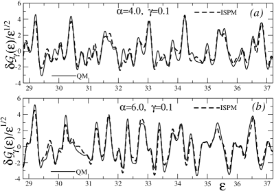
Figure 3: The oscillating part of the level density $\delta\mathcal{G}_{\gamma}(\varepsilon)$ in units of $\varepsilon^{1/2}$ vs the scaled energy $\varepsilon$ for $\alpha=4.0$ (a), and $\alpha=6.0$ (b), at the (dimensionless) width parameter $\gamma=0.1$ in the Gaussian averaging over the scaled energies; the solid and dashed curves are the quantum-mechanical and semiclassical ISPM results, respectively.

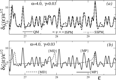
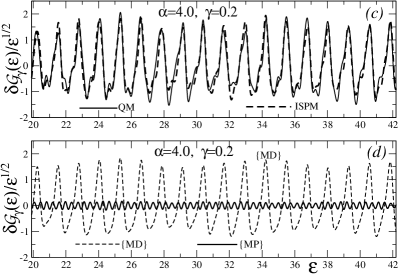
Figure 4: The same as in Fig. 3 for $\alpha=4.0$ but with other width parameters, $\gamma=0.03$ (a,b) and $\gamma=0.2$ (c,d). Panels (a,c): the solid, dashed and dotted lines are the QM, ISPM and SSPM [ the panel (a)] results. Panels (b,d): $\{MD\}$ (dashed) is the contribution of the diameters (including their repetitions) and $\{MP\}$ (thin solid) for other $\mathcal{K}=1$ polygon-like POs.

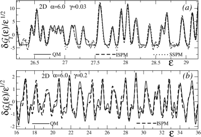
Figure 5: The same as in Fig. 3 for $\alpha=6.0$, but with other width parameters, $\gamma=0.03$ (a), and $\gamma=0.2$ (b).

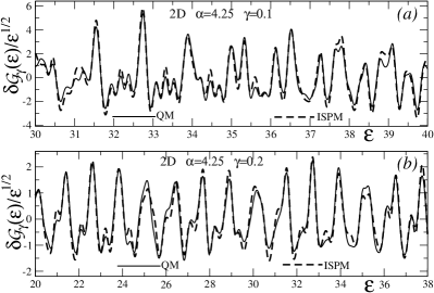
Figure 6: The same as in Fig. 5 for $\alpha=4.25$, but with the width parameters, $\gamma=0.1$ (a), and $\gamma=0.2$ (b).

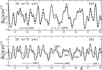
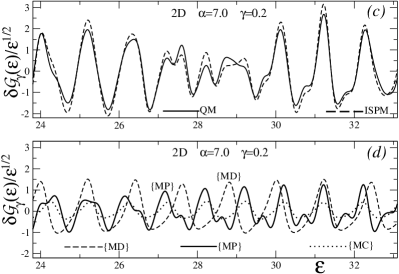
Figure 7: The same as in Fig. 4, but for $\alpha=7.0$ and other width parameters, $\gamma=0.1$ (a,b) and $\gamma=0.2$ (c,d).

Figures 3–7 show the oscillating part of the semiclassical scaled-energy level density $\delta\mathcal{G}_{\gamma}(\varepsilon)$ [Eq. (54)] in units of $\varepsilon^{1/2}$ as functions of the scaled energy $\varepsilon$ for several values of the power parameter $\alpha$ and the Gaussian width $\gamma$. The ISPM semiclassical results show good agreement with the quantum mechanical (QM) ones for a transition from the gross to fine resolutions of the spectra. The QM calculations are carried out by the use of the standard Strutinsky averaging over the scaled energy $\varepsilon$, in which we find a good plateau around the Gaussian averaging width ${\widetilde{\gamma}}=2-3$ with the even curvature correction polynomials of 4th to 8th powers.

For the powers $\alpha=4.0$ and $6.0$, one finds a good agreement with the SSPM asymptotic behavior [Figs. 4(a) and 5(a)] because they are sufficiently far from the bifurcation points $\alpha=4.25$ and $7.0$ which correspond to the birth of the star-like $(5,2)$ and triangle-like $(3,1)$ POs (Figs. 6 and 7). For the gross shell structure ($\gamma\approx 0.2$ at $\alpha=4.0$), only the shortest orbits (mainly a few shortest diameters) give the leading contributions. (This is in contrast to the 3D case where the circular orbits become also important trap ; book .) For instance, the gross shell structure in terms of the shortest POs for $\alpha=6.0-7.0$ manifests at larger $\gamma\gtrsim 0.3$, unlike for the powers $\alpha=4.0-4.25$. With decreasing $\gamma$ and increasing $\alpha$, the POs for larger scaled periods $\tau$ [or actions $S$, see Eq. (III.3)] become more significant [cf. Figs. 4(b,d) and 7(b,d)]. In the case of the fine shell structure (e.g., $\gamma\approx 0.03$) the dominant contributions are due to the bifurcating $\mathcal{K}=1$ POs [polygon-like POs denoted by $\{MP\}$; see Fig. 4(b)]. (This is similar to the situations in the elliptic ellipse and spheroidal spheroid cavities, and in the IHH potential maf .) However, the interference of these much longer one-parametric POs [such as $M(7,3)$ for $\alpha=4.0$ or $M(5,2)$ for $\alpha=6.0$] with a lot of the $M(2,1)$ diameters explain some peaks, too. For smaller $\alpha=4.0$ and $4.25$, the circle orbit contributions are not shown because they are insignificant at these power parameters in the 2D case. (This is different situation from the 3D case, see Ref. trap for the trace formulas based on the uniform approximation using the classical perturbation approach creagh96 ; book .) These contributions into the trace formula (54) are increasing functions of $\alpha$, and they become significant at $\alpha\gtrsim 7$ even for the 2D case [Fig. 7(b,d)]. An intermediate situation between the gross- and fine- shell structures where all of POs become significant are shown too at $\gamma=0.1$ in Figs. 3 and 6, and at $\gamma=0.1$ and $0.2$ in Fig. 7(b,d). Our full analytical expressions (accessible for any long periodic orbits) for the classical PO characteristics at $\alpha=4$ and $6$ are quite useful in the simple ISPM calculations of the oscillating level density with a good accuracy up to the fine spectrum-structure resolutions by using, for instance, $\gamma\approx 0.03$ and $0.1$. Figures 6 and 7 show a nice agreement of the fine-resolved semiclassical and quantum level densities $\delta\mathcal{G}_{\gamma}(\varepsilon)$ as functions of the scaled energy $\varepsilon$ at the critical bifurcation points $\alpha=4.25$ and $7.0$ for the births of the star-like $(5,2)$ and triangle-like $(3,1)$ orbits, respectively.

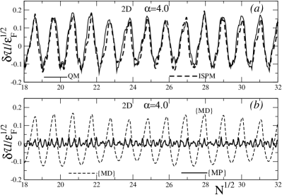
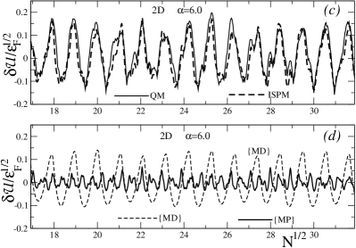
Figure 8: Scaled shell correction energies $\delta\mathcal{U}$, normalized by the factor $\varepsilon_{F}^{-1/2}$, as functions of square root of the particle number $N^{1/2}$ at the values of $\alpha$, where the full analytical formulas are obtained for $\alpha=4.0$ (a,b) and $\alpha=6.0$ (c,d). Panels (a,c): QM (solid curve) represents the quantum-mechanical results using the Strutinsky SCM, and ISPM (dashed curve) shows the semiclassical result using the TF approximation in the calculation of $N(\varepsilon_{F})$ by Eqs. (59) and (66). Panels (b,d): the contributions of several POs into the shell correction energy $\delta\mathcal{U}$ are shown. Other notations are the same as in Figs. 4 and 7.

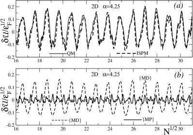
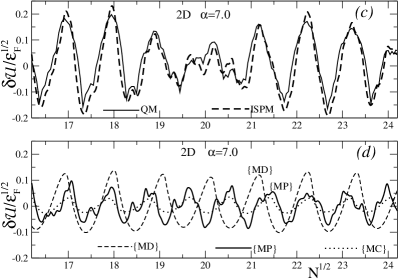
Figure 9: The same as in Fig. 8; $\alpha=4.25$ for the (5,2) bifurcation, and $\alpha=7.0$ for the (3,1) bifurcation are shown in panels (a,b) and (c,d), respectively.

Figures 8 and 9 show the scaled shell correction energies $\delta\mathcal{U}$ [Eqs. (58) for the semiclassical and (62) for the quantum results], normalized by the factor $\varepsilon_{F}^{-1/2}$, as functions of the particle number variable $N^{1/2}$. A good plateau is realized for the QM calculations of the scaled shell-correction energies [see the first equation in Eq. (62)] near the same averaging parameters ${\widetilde{\gamma}}$ and curvature corrections as mentioned above. In the semiclassical calculations, the Fermi level $\varepsilon_{{}_{\!F}}$ is determined by the particle number conservation (59) with using the coarse-grained scaled-energy POT level density,

$$\mathcal{G}_{\gamma,\;{\rm scl}}(\varepsilon)=\mathcal{G}_{\rm TF}(\varepsilon)+\sum_{\mathcal{K}=0}^{1}\delta\mathcal{G}^{(\mathcal{K})}_{\gamma,\;scl}(\varepsilon).$$ (66)

The oscillating ISPM components $\delta\mathcal{G}^{(\mathcal{K})}_{\gamma,\;scl}(\varepsilon)$ are given by Eqs. (54) and (48). We evaluated the Fermi level $\varepsilon_{{}_{\!F}}(N)$ by varying the averaging width $\gamma$ and found that there is no essential sensitivity within the interval of smaller $\gamma$ ($\gamma\approx 0.1-0.2$). Moreover, even the TF density $\mathcal{G}_{\rm TF}(\varepsilon)$ [Eq. (63] in Eq. (59) with $\mathcal{G}(\varepsilon)\approx\mathcal{G}_{\rm TF}(\varepsilon)$ provides us a good value of $\varepsilon_{{}_{\!F}}$ in the POT calculations of the shell correction energies (58). The PO sums at $\alpha=7.0$ converge for the shell correction density (54) by using the averaging width $\gamma=0.2$ of a fine shell-structure resolution, and for the shell correction energies (58) with taking into account the same major simplest POs [about 4 repetition numbers ($M=4$) for the circle and diameter orbits, and a few first simplest other $\mathcal{K}=1$ ($P$) POs, such as $(3,1)$, $(5,2)$, $(7,3)$ and $(8,3)$; cf. Figs. 9(c,d) with 7(c,d)]. For smaller diffuseness, $4\lesssim\alpha\lesssim 6$, one has a similar PO convergence relation with the same $\gamma\approx 0.2$, but with much smaller contributions of the circular orbits. However, the dominating ($\mathcal{K}=1$) PO families (P) are the $(5,2),(7,3)$ and $(7,3)$ POs at $\alpha=4.25-6.0$ and $4.0$, respectively [Figs. 8(a,b) and 4(c,d)]. As seen from Figs. 6, 7 and 9, we obtain a nice agreement between the semiclassical (ISPM, dashed) and quantum (QM, solid curve) results exactly at the bifurcations $\alpha=4.25$ and $7.0$. Notice that the dominating contributions in these semiclassical results at the bifurcation point $\alpha=7.0$ are coming from the interference of the bifurcating circle $C$ and newborn $(3,1)$ orbits with the simplest diameters. As shown typically in Figs. 7(d) and 9(d), one can see that the circle $C$ and triangle-like $(3,1)$ orbits are mainly in phase, but the diameter $(2,1)$ is sometimes in phase to them and sometimes out of phase. Thus, the occurrence of a characteristic beating pattern in the level density amplitude at $\alpha=7.0$ is due to the interference of the bifurcating orbits $C$ and $(3,1)$ with the shortest diameter $(2,1)$ having all the amplitude of the same order in magnitude but different phases. The bifurcating circle $2C$ and star-like $(5,2)$ orbits [as expected from the enhancement of the amplitudes of the circular $C$ and triangular-like $(3,1)$ POs in Fig. 2] are more important for $\alpha=4.25$, though the primitive diameters become significant much compared to the bifurcation case $\alpha=7.0$. The POs $(3,1)$ and $(5,2)$ yield more contributions near their bifurcation values of $\alpha$, and even more on the right-hand side ($\alpha\gtrsim\alpha_{\rm bif}$) in a wide region of $\alpha$ as mentioned above. The bifurcation parent-daughter partner orbits $\{C$, $(3,1)\}$ and $\{2C$, $(5,2)\}$, taken together with the simple diameter $(2,1)$, give essential ISPM contributions of about the same order of magnitude in Figs. 6, 7 and 9; as seen for example in Figs. 7(b,d) and 9(d) for the same $\alpha=7.0$. The diameter ISPM contributions are close to the SSPM asymptotic ones near the bifurcation points $\alpha=7.0$ and $4.25$ (as for $\alpha=4.0$ and $6.0$) because they are sufficiently far from their single symmetry-breaking point at the harmonic oscillator value $\alpha=2$.

Figure 10: Moduli of the Fourier transform $|F(\tau)|$ of the quantum scaled-energy level density (50) as functions of the dimensionless variable $\tau$ are plotted for several values of $\alpha$; $MC$ and $M(n_{r},n_{\varphi})$ indicate the classical POs corresponding to each peak (see Fig. 1).

Figure 10 shows the Fourier transform of the quantum-mechanical scaled-energy level density [Eq. (50)]. For a smaller $\alpha=2.1$, the diameter $(2,1)$ orbit gives the dominant contribution to the gross-shell structure as the shortest POs; see the peak at $\tau\sim 5.0$. With increasing $\alpha$, the amplitude of the circle orbit becomes again larger due to a prominent enhancement around the bifurcation point ($\tau\sim 6.2$ at $\alpha_{\rm bif}=7.0$). Notice that the newborn POs $(3,1)$, $(5,2)$, $(7,3)$ and $(8,3)$ give comparable contributions at $\alpha=7.0$ [similarly, $(5,2)$ and $(7,3)$ for the bifurcation $\alpha=4.25$] in nice agreement with the quantum Fourier spectra in Fig. 10. The contributions of the newborn triangle-like orbit family $(3,1)$ having relatively a smaller scaled period $\tau_{{}_{\!(3,1)}}$ and higher degeneracy $\mathcal{K}=1$ become important and dominating for larger $\alpha\gtrsim\alpha_{\rm bif}=7$. The newborn $(3,1)$ peak cannot be distinguished from the parent circle $C$ orbit near the bifurcation point $\alpha_{\rm bif}$ as well as the diameter and circle orbits at $\alpha$ close to the HO limit, see Ref. migdal . We emphasize that the shell correction energies $\delta\mathcal{U}$ are similar to the oscillating parts of the level densities coarse-grained over the spectrum by using the Gaussian width $\gamma=0.2$ at $\alpha=4.0$ and $4.25$, which have mainly the gross-shell structure due to the shortest diameters. However, for this $\gamma$, the fine-resolved shell structures (due to their interference with the other polygon-like and circular POs) are pronounced at larger powers near $\alpha=6.0$, and especially, $7.0$.

Notice also that we do not show the numerical comparison of the ISPM [Eqs. (54) and (58)] vs quantum (Ref. book ) results for the HO limit $\alpha\to 2$ because they are exactly coincide, as shown analytically around Eq. (65).

V Conclusions

We presented a semiclassical theory of quantum oscillations of the level density and energy shell corrections for a class of radial power-law potentials which turn out as good approximations to the realistic Woods-Saxon potential in the spatial region where the particles are bound. The advantage of the RPL potentials is that, in spite of its diffuse surface, the classical dynamics scaling with simple powers of the energy simplifies greatly the analytical POT calculations. The quantum Fourier spectra yield directly the contributions of the leading classical POs with the specific periods and actions into the trace formulas.

We described the main PO properties of the classical dynamics in the RPL potentials as the key quantities of the POT. Taking the simplest two-dimensional RPL Hamiltonian we developed the semiclassical trace formulae for any its power $\alpha$, and studied various limits of $\alpha$ (the harmonic oscillator potential for $\alpha=2$ and the cavity potential for $\alpha\to\infty$). The completely analytical results were obtained for the RPL powers $\alpha=4$ and $6$. This can be applied for both 2D and 3D cases and allow us to far-going fine-resolved shell structures at $\gamma=0.03-0.1$. This POT is based upon extended Gutzwiller’s trace formula, that connects the level density of a quantum system to a sum over POs of the corresponding classical system. It was applied to express the shell correction energy $\delta U$ of a finite fermion system in terms of POs. We obtained good agreement between the ISPM semiclassical and quantum-mechanical results for the level densities and energy shell corrections at several critical powers of the RPL potentials. For the powers $\alpha=4$ and $6$, we found also good agreement of the ISPM trace formulas with the SSPM ones. The strong amplitude-enhancement phenomena at the bifurcation points $\alpha=7$ and $4.25$ in the oscillating (shell) components of the level density and energy were observed in the remarkable agreement with the peaks of the Fourier spectra. We found a significant influence of the PO bifurcations on the main characteristics (oscillating components of the level densities and energy-shell corrections) of a fermionic quantum system. They leave signatures in its energy spectrum (visualized, e.g., by its Fourier transform), and hence, its shell structure. We have presented a general method to incorporate bifurcations in the POT, employing the ISPM based on the catastrophe theory of Fedoryuk and Maslov, and hereby, overcoming the divergence of the semiclassical amplitudes of the Gutzwiller theory and their discontinuity in the Berry&Tabor approach at bifurcations. The improved semiclassical amplitudes typically exhibit a clear enhancement near a bifurcation and on right side of it, where new orbits emerge, which is of the order $\hbar^{-1/2}$ in the semiclassical parameter $\hbar$. This, in turn, leads to the enhanced shell structure effects. Bifurcations are treated, again, in the ISPM leading to the semiclassical enhancement of the orbit amplitudes. The trace formulae are presented numerically to show good agreement with the quantum-mechanical level density oscillations for the gross- (coarse-grained with larger averaging width $\gamma$ and a few shortest POs), and the fine-resolved (with smaller $\gamma$ and longer bifurcating POs) shell structures. The PO structure of the shell-correction energies is similar to that of the coarse-grained densities for smaller powers $\alpha=4$ – $4.25$, and of the fine-resolved densities for larger $\alpha\gtrsim 6$ at the same $\gamma\approx 0.2$. The fine-resolved and coarse-grained shell structures were found at the same $\alpha$ in the corresponding averaged oscillating densities at smaller width parameters $\gamma=0.03$ – $0.1$ and at larger ones $\gamma\gtrsim 0.2$ – $0.3$, respectively. The fine-resolved shell structure for larger powers, $\alpha\gtrsim 6$, occurs in a larger interval, $\gamma=0.003$ – $0.2$, including the essential contributions of the circle orbits along with the polygon-like and diameter orbits. Full explicit analytical expressions for the diameters and circle orbit contributions into the trace formula as functions of the diffuseness potential parameter $\alpha$ are specified too.

For prospectives, we intend a further study of shell structures in the 3D RPL potentials, within the ISPM and uniform approximations to treat the bifurcations, by varying continuously the power parameter $\alpha$ from 2 (harmonic oscillator) to $\infty$ (spherical billiards).

Appendix A The stability factor, bifurcation powers and frequencies

Let us consider in more details the non-linear classical dynamics in the RPL Hamiltonian (2) for any real $\alpha\geq 2$. The critical values of the radial coordinate $r=r_{{}_{\!C}}$ and angular momentum $L=L_{C}$ for the circle orbit ($C$) are determined by the solutions of the system of the two equations with respect to $r$ and $L\;$:

$$\mathcal{F}(r,L)=0,\quad\frac{\partial\mathcal{F}}{\partial r}=0,\quad\text{where}\quad\mathcal{F}(r,L)\equiv p_{r}^{2}(r,L)\;,$$ (67)

see Eq. (4). In the internal region where the stable orbits in the radial direction exist, one has a nonzero $\mathcal{F}_{C}^{\prime\prime}=\partial^{2}\mathcal{F}\left(r_{{}_{\!C}},L_{C}\right)/\partial r^{2}<0$. First equation in Eq. (67) means that there is no radial velocity, $\dot{r}=0$, and the next equation is that the radial force is equilibrating by the centrifugal force. For the Hamiltonian (2), the solutions of the two these equations are the radius $r_{{}_{\!C}}$ and angular momentum $L_{C}$ aritapap ,

$$r_{{}_{\!C}}=R_{0}\left(\frac{2E}{(2+\alpha)E_{0}}\right)^{1/\alpha},\qquad L_{C}=p(r_{{}_{\!C}})r_{{}_{\!C}}\;.$$ (68)

Using Eq. (7) at $L=L_{C}$ for the rotational frequency, $\omega_{{}_{\!C}}=\omega_{\varphi}(L=L_{C})=L_{C}/(mr_{{}_{\!C}}^{2})$, and (68) for $r_{{}_{\!C}}$ and $L_{C}$, one finds aritapap

$$\omega_{{}_{\!C}}=\sqrt{\frac{\alpha E_{0}}{mR_{0}^{2}}}\,\left(\frac{2E}{(2+\alpha)E_{0}}\right)^{1/2-1/\alpha}\;.$$ (69)

Applying now the second order expansion in $r-r_{{}_{\!C}}$ to Eq. (4), one gets the first-order ordinary differential equation for the radial CT $r(t)$ locally near the circle PO $r=r_{{}_{\!C}}$:

$$\dot{r}=\pm\sqrt{\frac{\mathcal{F}_{C}^{\prime\prime}}{2m^{2}}}\,\left(r-r_{{}_{\!C}}\right)\;.$$ (70)

Integrating the dynamical equation in Eq. (70), one obtains

$$r(t)=r_{{}_{\!C}}+\left(r^{\prime}-r_{{}_{\!C}}\right)\,\,\exp\left(\pm\sqrt{\frac{\mathcal{F}_{C}^{\prime\prime}}{2\,m^{2}}}\,\,t\right)\;,$$ (71)

where $r^{\prime}=r\left(t=t^{\prime}=0\right)$. In the stable case, $\mathcal{F}_{C}^{\prime\prime}<0$ in Eq. (71) for the CT $r(t)$ locally near the circle orbit $r=r_{{}_{\!C}}$, one writes

$$r(t)=r_{{}_{\!C}}+\left(r^{\prime}-r_{{}_{\!C}}\right)\,\exp\left(\pm i\varOmega_{C}\,t\right)\;,$$ (72)

where $\varOmega_{C}$ is a positive radial frequency $\omega_{r}$ at $L=L_{C}$ [Eq. (7)],

$$\varOmega_{C}=\sqrt{\left|\mathcal{F}_{C}^{\prime\prime}/(2\,m^{2})\,\right|}=\omega_{r}(L=L_{C})\;.$$ (73)

For the Hamiltonian (2), this quantity is given by aritapap

$$\varOmega_{C}=\sqrt{\frac{2\alpha E}{mR_{0}^{2}}}\,\left[\frac{(2+\alpha)E_{0}}{2E}\right]^{1/\alpha}>0\;.$$ (74)

From Eq. (72) after the period $T_{C}$ along the primitive circle orbit,

$$T_{C}=t^{\prime\prime}-t^{\prime}=t^{\prime\prime}=\frac{2\pi}{\omega_{{}_{\!C}}}\;,$$ (75)

one finds

$$\delta r^{\prime\prime}\equiv r^{\prime\prime}-r_{{}_{\!C}}=\delta r^{\prime}\,\exp\left(\pm i\varOmega_{C}\,T_{C}\right),\quad\delta r^{\prime}=r^{\prime}-r_{{}_{\!C}}\;.$$ (76)

The eigenvalues of the stability matrix ${\cal M}_{C}$ for $M=1$ in Eq. (10) are given by book

$$\left(\frac{\partial r^{\prime\prime}}{\partial r^{\prime}}\right)_{p_{r}^{\prime}}\!\!=\exp{\left(i\varOmega_{C}\,T_{C}\right)},\quad\left(\frac{\partial p_{r}^{\prime\prime}}{\partial p_{r}^{\prime}}\right)_{r^{\prime}}\!\!=\exp{\left(-i\varOmega_{C}\,T_{C}\right)}\;.$$ (77)

These two eigenvalues of the stability matrix are complex conjugated in agreement with its general properties. As $\varOmega_{C}$ is real [$\varOmega_{C}>0$, according to Eqs. (73) and (74)] the circle orbit is isolated stable PO. Substituting the expressions (77) into the first equation in Eq. (10) and using Eqs. (75) for the period $T_{C}$, (69) and (74) for the C orbit frequencies $\omega_{{}_{\!C}}$ and $\varOmega_{C}$, relatively, one obtains the last equation in Eq. (10) for the stability factor $F_{MC}$.

Appendix B Scaling properties

For convenience, let us consider the classical dynamics in terms of the variables in dimensionless units $m=R_{0}=E_{0}=1$. Due to the scaling property (3) for the classical dynamics in the Hamiltonian (2), the energy dependence of the action $I_{r}(\varepsilon)$ [Eq. (5)], the angular momentum $L(\varepsilon)$, the frequency $\omega_{r}(\varepsilon)$ [Eq. (7)] and the curvature $K(\varepsilon)$ [Eq. (12)] can be expressed in terms of the simple powers of the scaled energy $\varepsilon$,

$$\varepsilon=E^{1/\alpha+1/2}\;.$$ (78)

In particular, one can express these classical quantities through their values at $\varepsilon=1$ ($E=1$),

$$I_{i}=I_{i}(1)\varepsilon,\quad L=L(1)\varepsilon,\quad\omega_{r}^{-1}=\omega_{r}^{-1}(1)\varepsilon^{(2-\alpha)/(2+\alpha)},$$

$$K=K(1)/\varepsilon\;.$$ (79)

Therefore, due to the scaling properties (3) and (79), we need to calculate these classical dynamical quantities only at one value of the energy $\varepsilon=1$. For simplicity of notations, we shall omit the argument $\varepsilon=1$ everywhere, if it is not lead to misunderstandings.

The radial action $I_{r}(L,E)$ [Eq. (5)] can be expressed explicitly in terms of the frequencies $\omega_{\varphi}$ and $\omega_{r}$ [Eq. (7)], and their ratio $f(L)$ [Eq. (9)],

$$I_{r}=\frac{2\alpha}{\alpha+2}\,\omega_{r}^{-1}-L\,f(L)\;.$$ (80)

To prove this identity, we express Eq. (7) for $\omega_{r}^{-1}$ in terms of the determinant,

$$\omega_{r}^{-1}=\frac{\partial(I_{r},L)}{\partial(E,L)}=\frac{\partial I_{r}}{\partial E}-\frac{\partial I_{r}}{\partial L}\;\frac{\partial L}{\partial E}\;.$$ (81)

Calculating directly the derivatives in this equation by using Eq. (79), one obtains the expression for $\omega_{r}^{-1}(1)$. Solving then this equation with respect to $I_{r}(1)$, one arrives at Eq. (80). Differentiating the identity (80) term by term over $L$ and using the definition for the ratio of frequencies $f(L)$ [Eq. (9)], for the curvature (12) one finally obtains

$$K =-\frac{2\alpha}{(\alpha+2)L}\;\frac{\partial\omega_{r}^{-1}}{\partial L}$$

$$=-\frac{\alpha}{\pi(\alpha+2)L}\;\frac{\partial T_{r}}{\partial L}\,,\quad T_{r}=\frac{2\pi}{\omega_{r}}\;.$$ (82)

According to Eqs. (7) and (9) with the help of Ref. byrdfried , $\omega_{r}^{-1}$ is obviously simpler quantity to differentiate over $L$ than $f(L)$,

$$\omega_{r}^{-1}=\frac{1}{2\pi\sqrt{2}}\,\int_{x_{\rm min}}^{x_{\rm max}}\frac{\mathrm{d}x}{\sqrt{Q(x,L,\alpha)}},$$ (83)

$$Q(x,L,\alpha)=\left(1-x^{\alpha/2}\right)\,x-L^{2}/2\;,$$ (84)

and $x=r^{2}$. The turning points $x_{\rm min}(L,\alpha)$ and $x_{\rm max}(L,\alpha)$ are determined by the equation:

$$Q(x,L,\alpha)=0\;.$$ (85)

Thus, we may calculate $\omega_{r}^{-1}$ and $f(L)$, and then, use Eqs. (80) and (82) for the radial action $I_{r}$, and curvature $K$ at the scaled energy $\varepsilon=1$. Then, one obtains their energy dependence through the scaling equations (78) and (79), respectively.

Appendix C Full analytical classical dynamics for powers 4 and 6

For the powers $\alpha=4$ and $6$, the roots of function (84), in particular, the turning points $x_{\rm min}$ and $x_{\rm max}$ can be obtained explicitly analytically. Therefore, one can find the explicit analytical expressions for the key quantities of the classical dynamics for the POT, namely, the radial frequency $\omega_{r}$ [Eq. (7)] (or the radial period $T_{r}$), and the frequency ratio $f(L)$ [Eq. (9)] in terms of the elliptic integrals from Ref. byrdfried (all in dimensionless units).

For $\alpha=4$, one has the cubic polynomial equation $Q(x,L,\alpha)\equiv x-x^{3}-L^{2}/2=0$ [Eqs. (84) and (85)] for the three roots $x_{\rm min}$, $x_{\rm max}$ and $x_{1}$; given by the Cardano formulas explicitly as functions of $L$ in the physical region $L\leq L_{C}$, $r_{1}<0\leq r_{\rm min}\leq r_{\rm max}$; $x_{q}=r_{q}^{2}$. For the radial period $T_{r}$ [Eqs. (82) and (7)], one obtains the analytical expression through these roots in terms of the complete elliptic integral $\mathrm{F}(\pi/2,\kappa)$ of the first kind trap ; byrdfried ,

$$T_{r}=\frac{2\pi}{\omega_{r}}=\frac{\sqrt{2}}{\sqrt{x_{\rm max}-x_{1}}}\;\mathrm{F}\left(\frac{\pi}{2},\kappa\right),$$ (86)

where $\kappa=[\left(x_{\rm max}-x_{\rm min}\right)/\left(x_{\rm max}-x_{1}\right)]^{1/2}\;$. For the ratio frequencies $f(L)$ [Eq. (9)], one finds

$$f(L)=\frac{L}{\pi\sqrt{2}\;x_{\rm max}\sqrt{x_{\rm max}-x_{1}}}\;\Pi\left(\frac{r_{\rm max}-r_{\rm min}}{r_{\rm max}},\kappa\right)\;,$$ (87)

where $\Pi(n,\kappa)$ is the complete elliptic integral of the 3rd kind byrdfried .

For $\alpha=6$, one has the polynomial equation of the 4th power, $Q(x,L,6)\equiv x-x^{4}-L^{2}/2=0$, having the 4 roots [two complex conjugated $x_{1}+ix_{2}$ and $x_{1}-ix_{2}$, and again, two real positive roots, $x_{\rm min}$ and $x_{\rm max}$; see Eqs. (84) and (85)]. The radial period $T_{r}$ is determined through these roots by the expression [similar to Eq. (86], see Refs. trap ; byrdfried ,

$$T_{r}=\frac{\sqrt{2}}{\sqrt{AB\left(x_{\rm max}-x_{1}\right)}}\;\mathrm{F}\left(\frac{\pi}{2},\kappa\right),$$ (88)

where $~{}\kappa=\{[(x_{\rm max}-x_{\rm min})^{2}-(A-B)^{2}]/(4\;AB)\}^{1/2}~{}$, $~{}A=[\left(x_{\rm max}-x_{1}\right)^{2}+x_{2}^{2}]^{1/2}~{}$,$~{}B=[(x_{\rm min}-x_{1})^{2}+x_{2}^{2}]^{1/2}\,$. (We reduced the 4-power polynomial equation to a cubic one and obtained its 4 analytically given roots, mentioned above, in the explicit Cardano’s form as functions of $L$). For $f(L)$ [Eq. (9)] at $\alpha=6$, one obtains byrdfried

$$f(L)=\frac{\sqrt{2}\;L\;(A+B)}{\pi\;\sqrt{AB}\left(Ax_{\rm min}-Bx_{\rm max}\right)}\;$$

$$\quad\times\left[\beta\;\mathrm{F}\left(\frac{\pi}{2}\kappa\right)+\frac{\beta-\beta_{1}}{2(1-\beta^{2})}\;\Pi\left(\pi,\frac{\beta^{2}}{1-\beta^{2}},\kappa\right)\right]\;,$$ (89)

where $\Pi(\varphi,n,\kappa)$ is incomplete elliptic integral of the 3rd kind, $~{}\beta=(Ax_{\rm min}-Bx_{\rm max})/(Ax_{\rm min}+Bx_{\rm max})~{}$, $\beta_{1}=(A-B)/(A+B)\;$. The curvatures $K$ [Eq. (82)] for $\alpha=4$ and $6$ are determined by taking analytically the derivative of the radial period $T_{r}$ [Eqs. (86) and (88)] over $L$ through the derivatives of the roots $x_{\rm min}(L)$, $x_{\rm max}(L)$, $x_{1}(L)$ and $x_{2}(L)$ for the derivative of $\mathrm{F}(\pi/2,\kappa)$ over $\kappa$ byrdfried . The expressions for the curvatures $K$ at the both powers $\alpha=4$ and $6$ can be found in the closed analytical form through a rather bulky formulas, which contain the complete elliptic integrals of the 1st and 2nd kind.

Appendix D Classical dynamics and boundaries for the diameters

For the primitive diameter $D=(2,1)$, the action $S_{D}$ (all in this appendix in dimensionless units) is specified analytically through the scaled period $\tau_{{}_{\!D}}$ and energy $\varepsilon$ by

$$S_{D}=\tau_{D}\varepsilon\;,\quad\tau_{{}_{\!D}}=\frac{4\sqrt{2\pi}}{\alpha+2}\;\Gamma\left(\frac{1}{\alpha}\right)\;\Gamma\left(\frac{1}{2}+\frac{1}{\alpha}\right)\;,$$ (90)

where $\Gamma(x)$ is the Gamma function of a real positive argument $x$. For the diameter PO boundaries, one can use the same $L_{-}=0$, but $L_{+}=b_{D}L_{C}$, where

$$b_{D}=1-\frac{1}{2}\;\exp\left[-\left(\frac{L^{HO}_{D}-L_{D}}{2\varDelta_{D}}\right)^{2}\right]$$ (91)

(see Ref. maf and more details in relation to the HO limit in Sec. III.5), $L_{D}=0\;$ is the stationary point, $L_{D}^{HO}=L_{C}/2=\varepsilon/(2\sqrt{2})\;$ is the upper angular momentum $L_{+}$ for the $D$ orbits in the limit $\alpha\to 2$, in which $b_{D}\rightarrow 1/2$. In the semiclassical limit $\varepsilon\gg 1$, one has $b_{D}\rightarrow 1$. $~{}\varDelta_{D}=(\pi Mn_{r}K_{D})^{-1/2}~{}$ is the Gaussian width of the transition region between these two asymptotic limits. The $D$ curvature for $\alpha\geq 2$ at $L=L_{D}$ is given by

$$K_{D}=\frac{\Gamma\left(1-1/\alpha\right)}{\varepsilon\sqrt{2\pi}\,\Gamma\left(1/2-1/\alpha\right)}\;.$$ (92)

This exact analytical expression for the curvature $K_{D}$ at any $\alpha$ was derived by using a power expansion in Eqs. (85) and (80) over the variable proportional to $L^{2}$ near $L=0$ up to the terms linear in $L^{2}$. The Maslov phase for the diameter orbit was determined by Eq. (26) at $n_{r}=2$ and $n_{\varphi}=1$. Note that for the limit $\alpha\rightarrow 4$, the general expressions for the period $\tau_{{}_{\!D}}$ and action $S_{D}$ [Eq. (90)], the Maslov index $\sigma_{D}$ [Eq. (26)] with the same asymptotic (SSPM) limit of the constant part of the phase $\phi^{(D)}_{d}=-\pi(4b_{D}-3)/4\rightarrow-\pi/4$, and the curvature $K_{D}$ [Eq. (92)] for the diameter $(2,1)$ are identical to those obtained in Ref. trap .

Appendix E The boundaries and curvature for circle orbits

For the arguments $\mathcal{Z}_{p}^{(\pm)}$ and $\mathcal{Z}_{r}^{(\pm)}$ of the error functions in Eq. (38), one originally has

$$\mathcal{Z}_{p,MC}^{(\pm)}=\sqrt{-\frac{i}{2\hbar}\,\mathcal{J}_{MC}^{(p)}}\,\left(p_{r}^{(\pm)}-p_{r}^{*}\right),$$

$$\mathcal{Z}_{r,MC}^{(\pm)}=\sqrt{-\frac{i}{2\hbar}\,\mathcal{J}_{MC}^{(r)}}\,(r^{(\pm)}-r_{{}_{\!C}}),$$ (93)

where $p_{r}^{*}=0$ is the stationary point, $p_{r}^{(\pm)}$ and $r^{(\pm)}$ are maximal and minimal classically accessible values of $p_{r}$ and $r$ as the finite integration limits for the corresponding variables. To express the integration boundaries (93) in an invariant form through the curvature $K_{C}$ (41), and stability factor $F_{MC}$ (10), one may use now the simple standard Jacobian transformations, and the definition of the angle variable $\varTheta_{r}^{\prime}$ as canonically conjugated one with respect to the radial action variable $I_{r}$ by means of the corresponding generating function. In these transformations, we apply simple linear relations: $~{}p_{r}^{\prime\prime}-p_{r}^{*}=\left(\partial p_{r}^{\prime\prime}/\partial L\right)^{*}\,\left(L-L^{*}\right)~{}$, and $~{}r^{\prime}-r^{*}=\left(\partial r^{\prime}/\partial\varTheta_{r}^{\prime}\right)^{*}\,\left(\varTheta_{r}^{\prime}-\varTheta_{r}^{*}\right)$, where we immediately recognize the Jacobian coefficients. Note that there is no crossing terms due to the isolated stationary point $I_{r}^{*}=0,\;\varTheta_{r}^{*}=0$ and to equations for the canonical transformations. At the stationary point for the isolated circle PO, one has $f(L_{C})=-(\partial I_{r}/\partial L)_{L=L_{C}}=-1/\sqrt{\alpha+2}$ [Eqs. (9), (69) and (73)]. For the transformation of the derivative $\partial r^{\prime\prime}/\partial\varTheta_{r}^{\prime}$, one can apply the Liouville conservation of the phase space volume for the canonical variables to arrive at $\partial r^{\prime\prime}/\partial\varTheta_{r}^{\prime}=(\partial I_{r}/\partial L)/(\partial p_{r}^{\prime}/\partial L)$ and $\left|\mathcal{J}_{\rm CT}(p^{\prime}_{r},p^{\prime\prime}_{r})\right|=|(\partial p_{r}^{\prime\prime}/\partial L)/(\partial p_{r}^{\prime}/\partial L)|=1$ at the PO conditions $r^{\prime}\to r^{\prime\prime}\to r_{{}_{\!C}},\,p_{r}^{\prime}\to p_{r}^{\prime\prime}\to 0$. Using also the Jacobian identity,

$$F_{MC}=-\mathcal{J}_{MC}^{(p)}\mathcal{J}_{MC}^{(r)}/\mathcal{J}_{MC}\left(p_{r}^{\prime},p_{r}^{\prime\prime}\right)\;,$$ (94)

one obtains Eq. (40) for the arguments of the error functions in Eq. (38).

The expression (41) for the $C$ curvature $K_{C}$ (in dimensionless units at $\varepsilon=1$) was obtained from expansion of $f(L)$ [Eq. (9)] as function of $L$ in powers of $L_{C}-L=\epsilon^{2}$ up to the 2nd order terms in $\epsilon$. For this purpose, by using standard perturbation theory, we have to solve first Eq. (85) for the turning points $r_{\rm min}$ and $r_{\rm max}$, [the integration limits in Eq. (9)] in the following general form ($r$ is taken below in units of $R_{0}$),

$$r_{\rm max} = r_{C}+c_{1}\epsilon+c_{2}\epsilon^{2}+c_{3}\epsilon^{3}+c_{4}\epsilon^{4}+\cdots,$$

$$r_{\rm min} = r_{C}-c_{1}\epsilon+c_{2}\epsilon^{2}-c_{3}\epsilon^{3}+c_{4}\epsilon^{4}+\cdots.$$ (95)

Existence of such form of the solutions follows from a symmetry of the equation (85) with respect to the change of the sign of $\epsilon$. Substituting these solutions into Eq. (85) for arbitrarily small $\epsilon$, one gets the system of the recurrent equations for the coefficients $c_{n}$. The solutions of this system up to the 4th order in a perturbation parameter $\epsilon$ is given by

$$c_{1}=\sqrt{\frac{L_{C}}{\alpha}},\quad c_{2}=-\frac{\alpha+1}{6}\,c_{1}^{2},\quad c_{3}=\frac{(\alpha-2)(2\alpha+5)}{72}\,c_{1}^{3},$$

$$c_{4}=-\frac{(\alpha+1)(4\alpha^{2}+8\alpha+13)}{1080}\,c_{1}^{4}\;,$$ (96)

and so on. We transform now the integration variable $r$ in the integral of Eq. (9) for $f(L)$ to $y$, $r=r_{{}_{\!C}}(1-y)$, such that

$$f(L)=-\frac{L-\epsilon^{2}}{\pi}\,\int_{y_{\rm min}}^{y_{\rm max}}\frac{\mathrm{d}y}{(1-y)\,\sqrt{Q(y,L,\alpha)}}\;.$$ (97)

Here, $Q(y,L,\alpha)$ is given by Eq. (84),

$$Q(y,L,\alpha)$$

$$\quad=2\,r_{C}^{2}\,\left[1-\frac{2}{\alpha+2}\,(1-y)^{\alpha}-L_{C}^{2}+2L_{C}\epsilon^{2}-\epsilon^{4}\right]$$

$$\quad\equiv(y_{\rm max}-y)(y-y_{\rm min})\mathcal{R}(y)\;,$$ (98)

$$y_{\rm max} =\bar{c}_{1}\epsilon-\bar{c}_{2}\epsilon^{2}+\bar{c}_{3}\epsilon^{3}-\bar{c}_{4}\epsilon^{4},$$

$$y_{\rm min} =-\bar{c}_{1}\epsilon-\bar{c}_{2}\epsilon^{2}-\bar{c}_{3}\epsilon^{3}-\bar{c}_{4}\epsilon^{4}\;,$$ (99)

where $\bar{c}_{n}=c_{n}/r_{{}_{\!C}}$. We use the last representation in Eq. (98), introducing a new function $\mathcal{R}(y)$ of the new variable $y$ to separate the singularities of the integrand in Eq. (97) due to the turning points. This integrand has to be integrated exactly by using a smooth function $\mathcal{R}(y)$ of $y$, which can be expanded in $y$ at $y=0$ up to the second order,

$$\mathcal{R}(y)=\mathcal{R}(0)+\mathcal{R}^{\prime}(0)y+\frac{1}{2}\mathcal{R}^{\prime\prime}(0)y^{2}+\cdots.$$ (100)

In order to get analytically the final result, we note that $y$ in this expansion is of the order of $\epsilon$, according to Eq. (99). Substituting then these expansions (99) and (100) into very right of Eq. (98), we expand their middle in $y$ at $y=0$ up to the 4th order. After the cancellation of $\epsilon^{2}$ from both sides, and simple algebraic transformations, one has

$$\mathcal{R}(0)=\frac{2L_{C}}{\overline{c}_{1}^{2}}\left[1+\epsilon^{2}\,\overline{c}_{2}\,\left(1-k_{2}\right)\right]+\mathcal{O}(\epsilon^{4}),\quad k_{2}=\frac{\overline{c}_{2}}{\overline{c}_{1}^{2}},$$

$$\frac{\mathcal{R}^{\prime}(0)}{\mathcal{R}(0)}=2k_{2}+\mathcal{O}(\epsilon^{2}),\quad\frac{\mathcal{R}^{\prime\prime}(0)}{\mathcal{R}(0)}=2k_{2}(3k_{2}+1)+\mathcal{O}(\epsilon^{2})\;.$$ (101)

For the calculation of the circle orbit curvature $K_{C}$, we obviously need only quadratic terms in $\epsilon$ [linear in ($L_{C}-L$)]. Therefore, one may neglect the $\epsilon^{2}$ corrections in the second and third lines of Eq. (101) because they are multiplied by $y\sim\epsilon$ and $y^{2}\sim\epsilon^{2}$ in the expansion (100), respectively. Substituting now expansions (99) and (100) into the integral over y in Eq. (97), and taking $\mathcal{R}(0)$ off the integral, one then expands to the second order all quantities of the integrand in $y\sim\epsilon$, except for $(y_{\rm max}-y)(y-y_{\rm min})$ under the square root (in the denominator) which can be integrated exactly. Taking remaining integrals as $\int{\rm}dyy^{n}/\sqrt{(y_{\rm max}-y)(y-y_{\rm min})}$ from $y_{\rm min}$ to $y_{\rm max}$ [Eq. (99)], and then, expanding finally $f(L)$ [Eq. (97)] in $\epsilon$, we find that the linear terms exactly disappear. It must be the case because $f(L)$ is an even function of $\epsilon$. Thus, the coefficient in front of $\epsilon^{2}$ with the expressions for $\overline{c}_{n}$ ($n=1,2,3$) from Eq. (96) is Eq. (41) for the curvature $K_{C}$. We can also use this perturbation method for calculations of the next order curvatures, for instance, $\partial^{3}I_{r}/\partial L^{3}$, which appears in expansion of the phase integral in the exponent up to the third order terms near the stationary points within a more precise (3rd-order) ISPM spheroid .

References

- (1) V. M. Strutinsky, Nucl. Phys. A 95, 420 (1967); A 122, 1 (1968).
- (2) M. Brack, J. Damgård, A. S. Jensen, et al., Rev. Mod. Phys. 44, 320 (1972).
-
(3)
M. C. Gutzwiller, J. Math. Phys. 12, 343 (1971);
Chaos in Classical and Quantum Mechanics (Springer, New York, 1990). -
(4)
V. M. Strutinsky, Nukleonika (Poland) 20, 679 (1975);
V. M. Strutinsky and A. G. Magner, Sov. J. Part. Nucl. 7, 138 (1976). -
(5)
M. V. Berry and M. Tabor, Proc. Roy. Soc. London,
Ser. A349, 101 (1976);
J. Phys. A 10, 371 (1977). - (6) S. C. Creagh and R. G. Littlejohn, Phys. Rev. A 44, 836 (1991); J. Phys. A 25, 1643 (1992).
- (7) V. M. Strutinsky, A. G. Magner, S. R. Ofengenden, and T. Døssing, Z. Phys. A 283, 269 (1977).
- (8) M. Brack, S. M. Reimann and M. Sieber, Phys. Rev. Lett, 79, 1817 (1997).
- (9) A. G. Magner, S. N. Fedotkin, K. Arita, and K. Matsuyanagi, Prog. Theor. Phys. 108, 853 (2002).
- (10) A. G. Magner, I. S. Yatsyshyn, K. Arita, and M. Brack, Phys. Atom. Nucl., 74, 1445 (2011).
- (11) M. Brack and R. K. Bhaduri, Semiclassical Physics (revised edition: Westview Press, Boulder, USA, 2003).
- (12) R. D. Woods and D. S. Saxon, Phys. Rev. 95, 577 (1954).
- (13) K. Arita, Int. J. Mod. Phys. E 13 191 (2004).
- (14) K. Arita, Phys. Rev. C 86, 034317 (2012).
- (15) S. M. Reimann, M. Persson, P. E. Lindelof, and M. Brack, Z. Phys. B 101, 377 (1996).
- (16) A. G. Magner, S. N. Fedotkin, K. Arita, et al., Prog. Theor. Phys. 102, 551 (1999).
- (17) A. G. Magner, K. Arita, and S. N. Fedotkin, Prog. Theor. Phys. 115, 523 (2006).
- (18) M. Brack, M. Ögren, Y. Yu, and S. M. Reimann, J. Phys. A 38, 9941 (2005).
- (19) K. Arita and M. Brack, J. Phys. A 41, 385207 (2008).
- (20) H. Schomerus and M. Sieber, J. Phys. A: Math. Gen. 30, 4537 (1997).
- (21) M. V. Fedoryuk, Comput Math. Math. Phys. 2, 145 (1962); 4, 671 (1964); 10, 286 (1970) (in Russian); ibid, The saddle-point method (Nauka, Moscow, 1977, in Russian).
- (22) M. P. Maslov, Theor. Math. Phys. 2, 30 (1970).
- (23) S. Reimann, M. Brack, A. G. Magner, et al., Phys. Rev. A 53, 39 (1996).
- (24) S. C. Creagh, Ann. Phys. (N.Y.) 248, 60 (1996).
- (25) P. F. Byrd and M. D. Friedman, Handbook of Elliptic Integrals for Engineers and. Scientists, (second edition, Springer-Verlag, New York, 1971).