Fragmentation dynamics of DNA sequence duplications

Abstract

Motivated by empirical observations of algebraic duplicated sequence length distributions in a broad range of natural genomes, we analytically formulate and solve a class of simple discrete duplication/substitution models that generate steady-states sharing this property. Continuum equations are derived for arbitrary time-independent duplication length source distribution, a limit that we show can be mapped directly onto certain fragmentation models that have been intensively studied by physicists in recent years. Quantitative agreement with simulation is demonstrated. These models account for the algebraic form and exponent of naturally occuring duplication length distributions without the need for fine-tuning of parameters.

A century has elapsed since the earliest reports of the evolutionary impact of gene duplicationtaylor . At the time there existed only a macroscopic and phenomenological conception of genetic material, but within the last decade static characterization of the finest details of the latter has become routine. Its dynamics, on the other hand, remains for the most part only indirectly accessible; ‘snapshots’of complete individual genomes at short time intervals are not yet practical, and dynamics must be inferred from their cumulative effect on representative genome sequences.

This dynamics is important because to a good approximation genome sequence determines, via natural selection, the fates of individuals and of species - but our understanding of how this happens is primitive. Contemporary lineages are our primary source of genome sequence, making it difficult to associate the presence or absence of most genomic features with their effects, if any, on an individual. Indeed, a primary goal of modern genomics is to determine if, when, and on what time scales the sequence evolution reflects selection.

Neutral models of sequence evolution - sequence dynamics that, on the time scales of interest, are independent of selection - underlie all methods that we know of to achieve this goal stone . When sequences common to two different organisms, or that appear multiply within the same genome, exhibit identity exceeding (falling short of) that expected on given model of neutral evolution, it is taken as evidence either that negative (positive) selection is acting on these sequences, or that the neutral model is flawed. As a given sequence fragment has some chance of exhibiting any excess or shortfall of identity within a neutral model, selection is inferred probablistically by studying frequencies of the levels of sequence identity within or between genomes stone . Thus, length distributions of similar or identical sequences have traditionally played a fundamental role in genomics and molecular genetics, and our interpretation of genomic sequence relies upon our understanding of these distributions.

The topic of this manuscript originates in an empirical observation of algebraic duplicated-sequence length distributions in a broad range of natural genomes miller_report ; halvak ; gao_miller ; taillefer_miller . In koroteev_miller2011 an empirical model of duplication was proposed that accounted for the observed algebraic distribution of duplicated sequence lengths in natural genomes, but relied on tuning the length distribution of the duplication source. Here we analytically derive and solve an alternative model for which no such tuning is required.

The action of duplication is to copy a sequence fragment and subsequently to insert it, or to substitute it for a same-sized sequence fragment, elsewhere in a chromosome graur . Standard models of sequence evolution also incorporate random, uncorrelated base substitution.

A chromosome consists of a string of $L$ bases chosen from a finite alphabet; in natural genomes the alphabet is typically represented by four bases A, G, C, and T; for simplicity and without loss of generality we use here a two base alphabet. The fundamental sequence element that we study is the the set of repeated sequences within the chromosome, counted in an algorithm-independent way. Specifically, we study ‘supermaximal repeats’ (or ‘super maxmers’): sequence duplications neither copy of which is contained in any longer sequence duplication within the chromosome taillefer_miller ; koroteev_miller2011 . From now on, we refer to a supermaxmer of length $m$ simply as an $m$-mer.

Within our models duplications occur with the rate $\beta$ per unit time: namely, a subsequence of the length $m$ is chosen randomly within the chromosome according to a predetermined source distribution $P(m)$ and is susbtituted for a sequence of length $m$ at another randomly chosen position in the chromosome. It was numerically demonstrated koroteev_miller2011 that for monoscale sources and certain power-law source distributions, the duplication length distribution attained a stationary state at long times.

We denote the ensemble-averaged number of $m$-mers at time $t$ as $f(t,m)$. For a monoscale source $P(m)=\delta_{c}(D-m)$ ($\delta_{c}$, Kronecker delta), we expect at stationarity that $f(t,m)$ will decay rapidly for $m>D$. There are two processes altering the number of $m$-mers: a new duplication of fixed length $D$ can fragment an existing $m$-mer or generate a new $m$-mers by fragmenting a longer $m$-mer; processes of higher order in $D/L$ are ignored, where $D,L>>1$ but $D<<L$.

The time dependence of $f$ can be represented by terms of the form $uf(t,m)$, $u$ being a coefficient describing the rate of creation or destruction of corresponding $m$-mers. An $m$-mer is annihilated when a newly created duplication of length $D$ overlaps with one of the sequences composing the $m$-mer; the rate of this event is $2(D+m-a)/L$, where $a$ is the length of a single base. Alternatively an $m$-mer may be created when a newly created duplication overlaps with an $m+k$-mer, $k>0$. The probability that a $m+k$-mer produces an $m$-mer is $4a/L$.

Supermaxmers may also be annihilated by base substitution. Substitution occurs with rate $\mu$ per time unit per unit length (in bases); duplication with rate $\beta$, measured in $1/$time unit. Then the balance equation takes the form

$$f(t+1,m)-f(t,m)=-2\left[\frac{m+D-a}{L}\beta+\mu m\right]f(t,m)+$$

$$+\left[\frac{4}{L}a\beta+4a\mu\right]\sum_{k=m+1}^{D}f(t,k)+2\beta\delta_{c}(D-m).$$ (1)

The dimensions of (1) are correct as we take $\Delta t=1$, as it is seen from lhs of the equation. The solution of (1) converges to a stationary one. To see this, take $\mu=0$, $\beta=1$, $a=1$ [base], and note that (1) may be represented in matrix form as $\vec{f}(t+1)=A\vec{f}(t)+\vec{\delta_{c}}$, where the matrix $A$ is such that $A_{ii}=2(1-(D+1)/L)$, $A_{ij}=4/L$ for $i<j$, and $A_{ij}=0$, for $i>j$, $i,j=1,2,\ldots D$; the vector $\vec{\delta}_{c}$ is $\delta_{D}=2$, $\delta_{i}=0$, $i<D$. The matrix is upper triangular and its eigenvalues are readily computed yielding $\lambda_{i}=1-\beta(D+(i-1))/L$. It is evident that $0<\left|\lambda_{i}\right|<1$ for all $i$, as we assumed $D<<L$ and $i=1,2,\ldots D$, and consequently, the iteration is guaranteed to converge. For $\mu\neq 0$ the eigenvalues have the form $\lambda_{i}=1-\beta\frac{i+D-1}{L}-\mu i$, thus the requirement of the convergence to a stationary state $\left|\lambda\right|<1$ yields (approximately) $D<<L$, $\mu\Delta\tau<1/D$, $\Delta\tau$ being a time step.

If some initial state $\vec{f}(0)$ is given and if we denote by $\vec{f}_{s}$ the limiting stationary state of the system, we can calculate $\vec{f}_{s}$ as follows

$$\vec{f}_{s}=\lim_{t\to\infty}\vec{f}(t)=\lim_{t\to\infty}\left[T\sum_{k=0}^{t-1}\Lambda^{k}T^{-1}\vec{\delta}+T\Lambda^{t}T^{-1}\vec{f}(0)\right]$$

$$=T\lim_{t\to\infty}\sum_{k=0}^{t-1}\Lambda^{k}T^{-1}\vec{\delta},$$ (2)

where $A=T\Lambda T^{-1}$ and $T$ diagonalizes $A$ and consists of eigen vectors of $A$. Further estimates show that $\vec{f}_{s}=LT\tilde{\Lambda}T^{-1}\vec{\delta}$, where, e.g., for the case $\mu=0$ we have $\tilde{\Lambda}_{ji}=1/(D+i-1))$, for $j=i$ and $\tilde{\Lambda}_{ji}=0$ when $j\neq i$. We may write down the exact stationary solution of the equation (1) in scalar form

$$f(m,D,L,\mu)=\left[\frac{D-(m-a)}{\beta\frac{D+(m-a)}{L}+m\mu}-2\frac{D-m}{\beta\frac{D+m}{L}+(m+a)\mu}\right.$$

$$\left.+\frac{D-(m+a)}{\beta\frac{D+(m+a)}{L}+(m+2a)\mu}\right],\quad m<D.$$ (3)

Obvious scaling wrt. $L$ is observed when $\mu=0$. Comparisons to the empirical model koroteev_miller2011 with (3) for $\mu\neq 0$ are presented in fig. 1.

Figure 1: Curves represent stationary states of the system described in the paper for various base substitution rates $\mu$ and corresponding analytic solutions of the system (1) for $\beta=1$. The chromosome length $L=10^{7}$; source length $D=1024$. Increasing base substitution rates exhibits a power-law tail with the exponent $-3$. Note also the match of amplitudes between simulations and solution.

It is evident that with increasing base substitution rate both simulations and the solution demonstrate power-law behavior with the exponent $-3$. To obtain this exponent from the solution (3) observe that $f$ in (3) is approximately represented as $g^{\prime\prime}(x)$, where $g(x)=(D-x)/(\beta\frac{D+x}{L}+\mu x)$. Then one obtains $f(m,D,L,\mu)\sim 1/(\beta\frac{D+m}{L}+m\mu)^{3}$. The peak observed in the left-hand side of the length distributions reflects that of a random sequence of the length $L$. High mutations conserve this random part of the distribution while duplications tend to distort the statistic. The maximum of the peak is located in the point $m=\log_{2}L$ for binary sequence. For the maximum length of supermaxmers in a random binary sequence there is an estimate $M_{L}\sim 2\log_{2}L$arratia which thus corresponds to the width of the peak.

For dynamics described by a power-law source $p(m)\sim 1/m^{\gamma}$ the characteristic scale $D$ is replaced by the first moment of the source. We also make all lengths dimensionless, dividing them by the length of $1$ base $a$ or by the first moment of the source $M_{1}$. Then, we have for probabilities of fragmentation $p(m)=1/(m^{\gamma}\phi_{1}(\gamma,N))$, where $\phi_{1}(\gamma,N)=\zeta(\gamma)-\zeta(\gamma,N+1)$, $L=Na$, and $\zeta(\gamma)$ is the Riemann zeta-function, $\zeta(\gamma,N+1)$ is the generalized zeta-function. The equation for a finite-size system with a power-law source can be obtained similarly to that for the monoscale source and has the form

$$\Delta f(t,m)=-2\left[\frac{1}{N}\sum_{r=1}^{N}\frac{m+r-1}{\phi_{1}(\gamma,N)r^{\gamma}}\beta+ma\mu\right]f(t,m)+$$

$$+\left[\frac{4}{N}\beta+4a\mu\right]\sum_{k=m+1}^{N}f(t,k)+2\beta\frac{1}{\phi_{1}(\gamma,N)m^{\gamma}},$$ (4)

and $m,r=1,2,\ldots,N$.

The structure of the source makes an analytic representation unwieldy; the solution of (4) as $t\to\infty$ was obtained numerically. The comparison of the solution with simulations is presented in fig. 2.

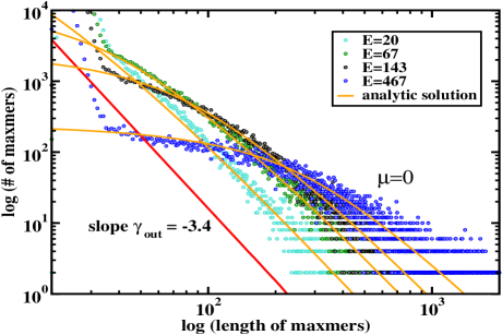
Figure 2: Curves represent stationary states of the system described in koroteev_miller2011 for various first moments $M_{1}$ of the power-law source of the form $p(\bar{x})\sim 1/(\bar{m}_{0}+\bar{x}^{\gamma})$ compared to the solution of (4). $L=10^{7}$, $\mu=0$, $\gamma=-2.4$. Deviation of solution from simulations is observed for small $M_{1}$, when the condition $M_{1}>>a$ is violated. For large lengths it is observed the regime with the exponent $\gamma+1$ described in koroteev_miller2011 . Values $\bar{m}_{0}$ corresponding to $M_{1}$ on the plot are: 10, 35, 75, 250.

.

Evidently equation (4) reproduces both exponent and amplitude and thus the dynamics involved encompasses both small and large mutation rates.

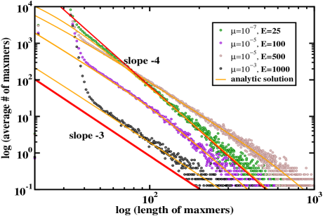
Figure 3: Curves represent stationary states of the system described in the Letter for $L=10^{7}$ and varying $M_{1}$ and $\mu$ compared to the solution of (4). The distributions are obtained by averaging over $100$ realizations. These are shown the regime $\mu^{-1}\approx M_{1}$ corresponding to the continuum equation and the regime with small mutation rate $\mu$ studied in koroteev_miller2011 , $\gamma=-3.0$.

.

Finally, some continuum limits following from these discrete dynamics are obtained. As all lengths are measured in bases we dimensionalize them as follows: $\bar{a}=a/M_{1}$, $\bar{m}=m/M_{1}$, $\bar{L}=L/M_{1}$, $\bar{t}=t\beta$, $\bar{\mu}=M_{1}\mu/\beta$. Then (4) with an arbitrary source $P(\bar{m})$ takes the form

$$\frac{\Delta f(t,m)}{\Delta t}=-2\left[\frac{1+\bar{m}-\bar{a}}{\bar{L}}+\bar{\mu}\bar{m}\right]f+$$

$$+\left[\frac{4\bar{a}}{\bar{L}}+4\bar{a}\bar{\mu}\right]\sum_{k=m+1}^{N}f+2P(\bar{m}).$$ (5)

Taking $\bar{a}\to 0$ and introducing densities $f=\bar{a}\hat{f}$, $P=\bar{a}\hat{p}$ with $\bar{L}=N\bar{a}$, $\bar{m}=n\bar{a}$, the equation becomes

$$\frac{\Delta\hat{f}(t,m)}{\Delta t}=-2\left[\frac{1+n\bar{a}-\bar{a}}{N\bar{a}}+\bar{\mu}\bar{a}n\right]\hat{f}+$$

$$+\left[\frac{4}{N\bar{a}}+4\bar{\mu}\right]\sum_{k=m+1}^{N}\hat{f}\bar{a}+2\hat{p}(\bar{m}).$$ (6)

Additionally, we introduce a duplication rate $\lambda$ measured per base taking $\beta=\lambda L$.

As $\bar{a}\to 0$ we assume $a<<M_{1}$, and as $\mu$ and $\lambda$ diminish with $a$, we need to evaluate the orders of corresponding terms. We keep the product $n\bar{a}$ finite and denote it by $x$; this implies $n\sim\bar{a}^{-1}$ and corresponds to an intermediate regimebarenblatt for (5). The source term has the order $\sim 1$. The main duplication term in (6) has the order $\sim\bar{a}^{\alpha-1}$, and mutation terms the order $\bar{\mu}\sim(\mu/\lambda)\bar{a}^{\alpha-1}$ as $\bar{a}\to 0$. We consider the case $\bar{\mu}\sim 1$, $\bar{a}^{\alpha-1}=o(1),\bar{a}\to 0$, other regimes being described elsewhere. Taking into account that in this regime $\bar{L}\to\infty$ and $L>>M_{1}$, the equation takes the form

$$\frac{\partial\hat{f}}{\partial\bar{t}}=-2x\bar{\mu}\hat{f}+4\bar{\mu}\int_{x}^{\infty}\hat{f}(\bar{t},y)dy+2\hat{p}(x)+O(\bar{a}^{\alpha-1}).$$ (7)

The main order regime corresponds to fragmentation with input studied in ben-naim .

For the numerical simulations in fig. 1 we set $L=10^{7}$, $M_{1}=D\approx 10^{3}$ and vary $\mu$; thus, $L>>M_{1}$. As $\mu$ approaches $10^{3}$ the output distribution approaches an algebraic form with exponent $-3$, corresponding to the solution of the fragmentation equation for a monodisperse sourceben-naim ; krapivsky . Fig. 2 corresponds to the regime with vanishing $\mu$ and is not described by (7); fig. 3 demonstrates various regimes and exponent $-3$ which is observed for $M_{1}>>a$, $\bar{a}^{\alpha-1}=o(\bar{\mu})$ and $m<<M_{1}$.

In fig. 4 we provide comparison of natural data with our simulations. Both chromosomes, one from human and the other from grapevine, demonstrate good fit to $-3$ that is also reproduced by our models.

From (6) and (7) it also follows that the duplications in this regime are dilute: a duplicated sequence is broken down by substitutions long before there there is any opportunity for a subsequent duplication to overlap with it. In this sense each $m$-mer evolves independently of other $m$-mers. Therefore, following Ben-Naim ben-naim we can estimate the fragment length distribution by following a typical duplication of length $M_{1}$. Substitutions break the duplication into fragments whose number $\mathcal{M}$ varies in time as $\mathcal{M}=M_{1}\mu t$ so that the average fragment length at time $t$ is $\langle m\rangle=M_{1}/\mathcal{M}$. Consecutive mutations are independent, hence the distribution of fragment lengths is close to Poisson for $\bar{a}<<1$, i.e., $p(m)\sim m^{-1}\exp(-m/\langle m\rangle)$, neglecting contributions exponentially in $M_{1}$. Then the number $S(t,m)$ of fragments of length $m$ is $\mathcal{M}p(m)$. New duplications occur continuously, so to obtain the fragment length distribution as $t\to\infty$ we integrate over time to obtain

$$S(m)=\int_{0}^{\infty}\mathcal{M}\beta p(m)dt\sim\int_{0}^{\infty}\frac{\mathcal{M}\beta}{m}e^{-m/\langle m\rangle}dt=\frac{M_{1}\beta}{\mu m^{3}}.$$ (8)

The similar result can be also obtained from the exact solution of (7) to give $S(m)=2M_{1}\beta/(\mu m^{3})$; the additional prefactor $2$ appears as in the equations for each sequences we count another one, which is identical to the former. The consistency of dimensions follows from the presence of additional prefactor $a$, which is equal to $1$ for the discrete case.

The estimate allows to calculate $M_{1}$ from the empirical distributions, e.g., for fig. 1 $\beta=1$, $\mu=10^{-4}$ in the algebraic regime. Then we can estimate $S(m)$ for $m=1$ from the plot supplemental (supplemental figure 1)); we have $S(m)\approx 2\times 10^{7}$ and from (8) we find $M_{1}\approx 10^{3}$ which pretty well corresponds to the real value $M_{1}=1024$ for this simulation. Similar estimates can be obtained for different sources.

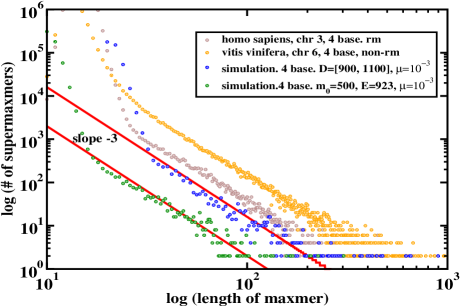
Figure 4: Human chr. 3 (brown) was repeat-masked, grapevine (orange) was not. Source length distributions were chosen as power-law with exponent $-2.4$ (green); and uniform on the interval $[900,1100]$ (blue). The latter was shifted along $x$ axis to the right by the factor of $2$ for clarity. Straight lines with the slope $-3$ have the amplitudes $2M_{1}\beta/\mu$ in accordance with (8) and the exact solution of (7). For the human chr. 3 we have $2M_{1}\beta/\mu\approx 3\times 10^{7}$, and for vitis vinifera chr. 6, $\approx 10^{8}$.

For eukaryotes, gene duplicatons are conventionally estimated to arise at around $\sim 10^{-2}$ per gene per $10^{6}y$ (years)lynch ; assuming $\sim 10^{4}$ genes per eukaryotic genome yields a genome-wide gene duplication ratelynch $\beta_{0}=10^{2}/10^{6}y$. Thus for the human genome with around $4\times 10^{4}$ genes, $\beta_{0}\approx 300/10^{6}y$lynch . Then, for duplication rate per base we have $\lambda_{0}=\beta_{0}/L_{0}$, where $L_{0}$ the number of bases belonging to genes; accepting the estimate $L_{0}$ to be $2\%$ of $L$ we can estimate $\lambda_{0}$. Let us assume that duplications, as well as point substitutions, are uniform over genome, i.e., duplication rate per base $\lambda=\lambda_{0}$ and for $\beta$ we have $\beta\approx 50\beta_{0}$. The average time between duplications, $1/\beta=200y$ corresponds to a single time unit in the parametrization of our models. The point substitution rate is $\mu\sim 10^{-2}$ per base per $10^{6}y$lynch or $\sim 10^{-5}$ per base per time unit. The algebraic regime with exponent $-3$ is already attained for $\mu=10^{-5}$ in fig. 1 and $\mu/\lambda=100>>1$ for this simulation.

To give estimates of time of emerging of currently observed identical repeats in human genome we use repeat-masked chr. 3 (Supplemental figure 2). With estimates and assumptions given above we find $\lambda\approx 0.5\times 10^{-5}$ per base, per $10^{6}$ y and consequently $\beta\approx 0.5\times 10^{3}$ (we take into account here that the length of repeat-masked chromosome differs significantly from that of the whole sequence). Then, we find $M_{1}\approx 300$, the average duplication length in human chr. 3. Note also, that the tail drops off at this length supplemental (supplemental figure 2). Thus $M_{1}\beta\approx 1.5\times 10^{5}$ bases related to supermaxmers were duplicated in human genome per $10^{6}$ years. The region of the tail in supp. fig. 2 corresponds to lengths $m>30$; the tail contains $\approx 10^{6}$ bases, hence, assuming similar processes in different chromosomes, the observed long identical duplicates occurred in the human genome last $6-7$ million years. This estimate fairly well corresponds to divergence time between human and chimp.

A $-3$ exponent of distributions is observed in many natural genomestaillefer_miller . It is important to stress that this regime is reproduced by koroteev_miller2011 as well as by the model suggested here, which incorporates koroteev_miller2011 as a specific case. This regime is, in part, detected when stationary solutions of the equations (1) and (4) become weakly dependent on a duplication source, demonstrating at the same time algebraic form with the slope $-3$. Thus the state of many currently studied genomes mapped to this regime of our dynamics, may be understood as a result of continuous interaction of point substitutions and (segmental) duplications generated by some source. These results also provide some evidence for the neutral nature of long segmental duplications. On the other hand, the assumptions for (6) may be altered to obtain different regimes to include genomes, whose state deviates from $-3$ regime, e.g., because of extensive recent duplications.

As our manuscript was in final stages of revision, we learned of ardnt where a similar dynamics to that studied here was introduced.

Compared to ardnt we derive continuum dynamics directly and show how the crucial parameter $M_{1}$ (or $D$), the first moment of the source, appears in calculations to determine the regime in which we observe genomes with the exponent $-3$ for the length distribution.

In addition, our dynamics treats a broader problem in two respects: 1) we introduce and demonstrate the dependence of the observed regime in length distributions on $M_{1}$ as there is only one specific regime with the exponent $-3$ in which the first moment $M_{1}$ turns out to be less important; 2) our dynamics allows to consider various asymptotic orders of $\mu/\lambda$, not necessarily $\mu>>\lambda$.

Thus, $-3$ is observed in (7) asymptotically as $x\to 0$, corresponding to $m<<M_{1}$ for discrete equations (1), (4), i.e., the algebraic regime with the exponent $-3$ in natural genomes may be observed for duplicate lengths $<<M_{1}$. If the source produces short duplicates, which are in the same time are not hit by strong mutations (e.g., $\mu\sim\lambda$) then the tail occurs for $m>>M_{1}$ or in asymptotic regime $x\to\infty$ for (7) and we may observe regimes with different exponents (fig. 3) or even non-algebraic regimes. The latter ones are also observed in real genomes supplemental (supplemental figure 3) and can not be treated in terms of specific $-3$ exponent but are reproduced by our dynamics. Thus we can map various asymptotic regions of parameters to natural sequences to fit our observations in genomes, demonstrating variety of length distributions for duplicates.

We acknowledge Kun Gao, Eddy Taillefer and Satish Venkatesan for helpful duscussion of this work. We thank Quoc-Viet Ha for the help with computations. We also thank Peter Arndt, Florian Massip, Nick Barton, Daniel Weissman, and Tiago Paixao for discussions of this work and the manuscript.

References

- (1) reviewed in S. Taylor and J. Raes, Ann. Rev. Genet., 38:615 (2004).
- (2) E.A. Stone, G.M. Cooper, A. Sidow, Ann. Rev. Gen. Hum. Genet. 6:143 (2005).
- (3) J. Miller, IPSJ SIG Technical Report No. 2009-BIO-17(7):1 (2009).
- (4) W. Salerno, P. Havlak, J. Miller, Proc. Nat. Acad. Sci. USA, 103:13121 (2006).
- (5) E. Taillefer and J. Miller, in Proceedings of International Conference on Natural Computation, Shanghai, China, 2011, Vol. 3 (IEEE, New York, 2011), pp. 1480–1486; E. Taillefer, Miller, Int. Conf. on Computer Engineering and Bioinformatics, Cairo, Egypt, pp. 22–29, 2011.
- (6) K. Gao and J. Miller, PLoS One 6(7), (2011).
- (7) M.V. Koroteev, J. Miller. Scale-free duplication dynamics: A model for ultraduplication. Phys. Rev. E 84(061919), 2011
- (8) D. Graur, W.-H. Li. Fundamentals of molecular evolution. Sinauer, 2000
- (9) E. Ben-Naim, P.L. Krapivsky, Phys. Lett. A, 293(48), 2000. See also E. Ben-Naim, P.L. Krapivsky, J. of Statistical Mechanics theory and experiment, DOI: 10.1088/1742-5468/2005/10/L10002, 2005.
- (10) R. Arratia, M.S. Waterman, Ann. Prob. 13, 1236(1985).
- (11) P.L. Krapivsky, S. Redner, E. Ben-Naim. A kinetic view of statistical physics, Cambridge Univ. Press, 2010.
- (12) G.I. Barenblatt. Scaling, self-similarity, and intermediate asymptotics. Cambridge Univ. Press, 1996.
- (13) Supplemental materials
- (14) M. Lynch, J.S. Conery, Science 290(2000), 1151-1155; Science, 293(2001), p. 1551.
- (15) J.A. Bailey, E.E. Eichler, Nat. Rev. Genet., 7(2006), 552-556.
- (16) F. Massip, P.F. Arndt, PRL 110(2013), 148101.