A sensitivity analysis of the WFCAM Transit Survey for short-period giant planets around M dwarfs

Abstract

The WFCAM Transit Survey (WTS) is a near-infrared transit survey running on the United Kingdom Infrared Telescope (UKIRT), designed to discover planets around M dwarfs. The WTS acts as a poor-seeing backup programme for the telescope, and represents the first dedicated wide-field near-infrared transit survey. Observations began in 2007 gathering J-band photometric observations in four (seasonal) fields. In this paper we present an analysis of the first of the WTS fields, covering an area of 1.6 square degrees. We describe the observing strategy of the WTS and the processing of the data to generate lightcurves. We describe the basic properties of our photometric data, and measure our sensitivity based on 950 observations. We show that the photometry reaches a precision of $\sim 4$ mmag for the brightest unsaturated stars in lightcurves spanning almost 3 years. Optical (SDSS $griz$) and near-infrared (UKIRT $ZYJHK$) photometry is used to classify the target sample of 4600 M dwarfs with J magnitudes in the range 11–17. Most have spectral-types in the range M0–M2. We conduct Monte Carlo transit injection and detection simulations for short period ($<$10 day) Jupiter- and Neptune-sized planets to characterize the sensitivity of the survey. We investigate the recovery rate as a function of period and magnitude for 4 hypothetical star-planet cases: M0–2$+$Jupiter, M2–4$+$Jupiter, M0–2$+$Neptune, M2–4$+$Neptune. We find that the WTS lightcurves are very sensitive to the presence of Jupiter-sized short-period transiting planets around M dwarfs. Hot Neptunes produce a much weaker signal and suffer a correspondingly smaller recovery fraction. Neptunes can only be reliably recovered with the correct period around the rather small sample ($\sim 100$) of the latest M dwarfs (M4–M9) in the WTS. The non-detection of a hot-Jupiter around an M dwarf by the WFCAM Transit Survey allows us to place an upper limit of 1.7–2.0 per cent (at 95 per cent confidence) on the planet occurrence rate.

1 Introduction

M dwarfs are the most numerous stars in our Galaxy (Chabrier, 2003), and until recently have remained relatively unexplored as exoplanet hosts. While several hundreds of transiting exoplanets have been discovered around F,G and K dwarfs, only $\sim 70$ such planets are known around the lower mass M stars. M dwarfs make interesting targets for many reasons, for example they provide better sensitivity to smaller (rocky) planets in the habitable zone, and they also provide strong constraints on planetary formation theories.

The most successful techniques so far used to discover exoplanets are the radial velocity (RV) and transit methods. A planet around an early M2 dwarf can have $\sim$4 times deeper transits and $\sim$1.5 times higher RV amplitudes at the same orbital period than orbiting a Sun-like star. Both methods also show increasing sensitivity towards smaller semi-major axis. Around solar-type stars, planets in short period orbits (days) are extremely hot (above 1000K). If M dwarfs harbour planets in equally close-in orbits, they will probably be more interesting due to their moderate equilibrium temperatures. In case of later (M4-9) type M dwarfs, these planets may fall in the star’s habitable zone, and for rocky planets water can exist as a liquid, while Neptune-like planets may have water vapour in their atmospheres.

M dwarfs are also important for testing planet formation theories. In the core accretion paradigm, dust particles in the protoplanetary disk coagulate and form solid cores. The cores then begin to accumulate gas from the disk. When cores reach several Earth masses, gas accumulation can speed up significantly. It was first shown by Laughlin, Bodenheimer & Adams (2004) that gas giants cannot form easily around low mass stars this way. In the core accretion process gas giant formation is inhibited by time scale differences. The protoplanetary disk around a low mass host dissipates before planetary cores are able to accrete their gas envelope by entering the runaway gas accretion phase. These planets remain ‘failed cores’. Ida & Lin (2005) found very similar results. Newer models refine this picture by introducing more detailed relations between stellar and disk properties. They consider migration driven by disk-planet interactions (type I-II) (Ida & Lin, 2008), evolution of snow-line location (Kennedy & Kenyon, 2008) and planet-planet scattering (Thommes, Matsumura & Rasio, 2008). Their conclusions allow gas giant formation around low mass stars but the predicted frequency of giants systematically decreases towards lower primary masses. Kennedy & Kenyon (2008) give relative ratios for gas giant planets: a fraction of 1 per cent of low mass stars is predicted to have at least one giant planet, assuming that this ratio is 6 per cent for solar mass ones.

Due to the failed core outcome, it is not surprising that Neptunes and rocky planets are predicted to be common around low mass stars in core accretion models. Ida & Lin (2005) predict the highest frequency around M dwarfs for a few Earth mass planets in close-in orbits ($<$0.05 AU). Later models also firmly support the existence of these smaller planets (Ida & Lin, 2008; Kennedy & Kenyon, 2008).

Even if it is hard to form giant planets via core accretion around the lowest mass stars, gravitational instability models can produce gas giants on a very short timescale ($\sim 10^{3}\mathrm{yr}$). They predict that gas giants can form around low mass primaries as efficiently as around more massive ones assuming that the protoplanetary disk is sufficiently massive to become unstable (Boss, 2006).

(Wright et al., 2012, and references therein) give a summary of occurrence rates of hot giant planets ($T<10$ days) around solar G type dwarfs. RV studies determined a rate of 0.9–1.5 per cent (Marcy et al., 2005; Cumming et al., 2008; Mayor et al., 2011; Wright et al., 2012), while transit studies have a systematically lower rate (roughly half of this value) at 0.3–0.5 per cent (Gould et al., 2006; Howard et al., 2012, H12 hereafter).

For M dwarfs, recent RV studies support the paucity of giant planets (Cumming et al., 2008; Johnson et al., 2007, 2010; Rodler et al., 2012) though there are confirmed detections both with short- and long-period orbits. Johnson et al. (2007) found 3 Jovian planets (with orbital periods of years) in a sample of 169 K and M dwarfs, in the California and Carnegie Planet Search data. The planetary occurrence rate for stars with M$<0.7$M_⊙ in their survey is 1.8 per cent, which is significantly lower than the rate found around more massive hosts (4.2 per cent for Solar-mass stars, 8.9 per cent around higher mass subgiants). The positive correlation between planet occurrence and stellar mass remains after metallicity is taken into account, although at somewhat lower significance. Gravitational microlensing programmes also detected Jupiter-like giants around M dwarfs (e.g. Gould et al. (2010); Batista et al. (2011)) but statistical studies seem to arrive at different conclusions. Microlensing surveys are more sensitive to longer period systems than RV (and particularly transit) surveys. Gould et al. (2010) analyzed 13 high magnification microlensing events with 6 planet discoveries around low mass hosts (typically $0.5M_{\oplus}$) and derived planet frequencies from a small but arguably unbiased sample. They compared their planet frequencies to the Cumming et al. (2008) RV study. They found that after rescaling with the snow-line distance to account for their lower stellar masses in the microlensing case, the planet frequency at high semi-major axes is consistent with the distribution from the RV study extrapolated to their long orbits. They found a planet fraction at semi-major axes beyond the snow line to be 8 times higher than at 0.3 AU. Considering that hot giants in RV discoveries (around solar type stars) are thought to have migrated large distances into their short orbits, they conclude that giant planets discovered at high semi-major axes around low mass hosts do not migrate very far. Their study suggests that rather than the formation characteristics, the migration of gas giants may be different in the low mass case.

Focusing again on giant planets with short orbital periods around M dwarfs, then as of writing, there is only one confirmed detection. The Kepler Mission (Borucki et al., 1997), includes a sample of 1086 low-mass targets (in Q2) (Borucki et al., 2011, H12) and one confirmed hot Jupiter (P=2.45 days) around an early M dwarf host (KOI-254) (Johnson et al., 2012). Unfortunately, this object was not included in the statistical analysis of H12 study.

For transit surveys, sufficiently bright M dwarfs make good targets because of their smaller stellar radius. A Neptune-like object in front of a smaller host can produce a similar photometric dip ($\sim 1$ per cent) as a Jupiter-radius planet orbiting a Sun-like star. Ground based surveys are therefore potentially sensitive to planets around M dwarfs that could not be detected around earlier type stars with typical ground-based precision. On the other hand, M dwarfs provide a more demanding technical challenge. They are intrinsically faint and their spectral energy distribution peaks in the near infrared. Their faintness at optical wavelengths also makes spectroscopic follow-up observations difficult. Measuring photometry in the infrared helps, but introduces a higher sky background level. It is also worth pointing out that the intrinsic variability of M dwarfs (flaring, spots) could further reduce the ease of discovering transiting systems.

One approach is to target a large number of M dwarfs, with a wide-field camera equipped with optical or near-infrared detectors. An alternative approach is to target individual brighter M dwarfs in the optical deploying several small telescopes. Up till now, only 2 transiting planets have been discovered around (bright) M stars (Gillon et al., 2007; Charbonneau et al., 2009) by ground based transit surveys.

In this paper, we discuss the UKIRT (United Kingdom Infra Red Telescope) WFCAM (Wide Field CAMera) Transit Survey (WTS), the first published wide-field near-infrared dedicated programme, searching for short period ($<$10 day) transiting systems around M dwarfs. The survey was designed to monitor a large sample ($\sim 10,000$) of low-mass stars with precise photometry. In this paper we present an analysis of the first completed field in the WTS. We demonstrate that we can already put useful constraints on the hot Jupiter planet occurrence rate around M dwarf stars, and this is currently the strictest constraint available.

The survey observing strategy is described in Section 2. In Section 3 a summary is given of the data processing pipeline, describing the generation of final clean lightcurves from raw exposures. In Section 4 we describe the M dwarf sample and discuss uncertainties in classification. We evaluate the sensitivity of the survey in Section 5 using transit injection and detection Monte Carlo simulations. The lack of giant planets detected by the survey around M dwarfs to date is discussed in Section 6. Finally, in Section 7, we consider the H12 sample and use it to place an upper limit on the frequency of hot Jupiters around M dwarfs based on the Kepler Q2 data release. We discuss our WTS results in the context of both the Bonfils et al. (2011) and H12 studies.

2 The WFCAM Transit Survey

UKIRT is a 3.8m telescope, optimized for near-infrared observations and operated in queue-scheduled mode. The Minimum Schedulable Blocks are added to the queue to match the ambient conditions (seeing, sky-brightness, sky transparency etc). The WTS runs as a backup programme when observing conditions are not good enough (e.g. seeing $>$ 1 arcsec) for main surveys such as UKIDSS (Lawrence et al., 2007).

The Wide Field Camera (WFCAM) comprises four Rockwell Hawaii-II PACE arrays, with 2k$\times$2k pixels each covering 13.65 arcmin x 13.65 arcmin at a plate scale of 0.4 arcsec/pixel. The detectors are placed in the four corners of a square with a separation of 12.83 arcmin between the chips. This pattern is called a pawprint.

The WTS time series data are obtained in the J band ($\lambda_{\mathrm{eff}}=1220\ \mathrm{nm}$), the fields were also observed once in all other WFCAM bands (Z,Y,H,K) at the beginning of the survey. This photometric system is described in Hodgkin et al. (2009). Each field, covering 1.6 square degrees, is made up of an 8 pawprint observation sequence with slightly overlapping regions at the edges of the pawprints (Fig. 1). Observations are carried out using 10s exposures in a jitter pattern of 9 pointings. A complete field takes 16 min to complete forming the minimum cadence of the survey. Observing blocks typically comprise 2 or 4 repeats of the same field.

Four distinct WTS survey fields were chosen to be reasonably close to the galactic plane to maximize stellar density while keeping giant contamination and reddening at an acceptable level (see Section 4). The four fields are distributed in right ascension at 03, 07, 17 and 19 hours to provide all year coverage (at least one field is usually visible). At the time of the analysis presented in this paper, the 19 hour field has approximately 950 epochs which is close to completion (the original proposal requested 1000 exposures for each field), the other three are less complete. A summary of the key properties of the survey regions is shown in Table 1.

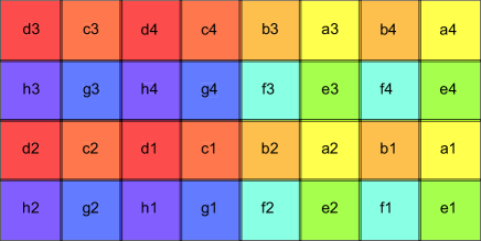
Figure 1: Observation pattern for the WTS. A field of 1.6 square degrees consists of 8 pawprints (a-h), each pawprint is built up from the simultaneous exposures of the four (numbered) detectors. The X-axis is Right Ascension, and increases to the left of the figure, while the Y-axis is Declination, and increases to the top.

name coordinates galactic No. of objects stellar RA, DEC l,b epochs ($J<17$) objects (h),(d) (d),(d) 19 19.58+36.44 70.03+07.83 950 69161 59270 17 17.25+03.74 24.94+23.11 340 17103 15343 07 07.09+12.94 202.89+08.91 350 24153 21224 03 03.65+39.23 154.99-12.99 240 17221 15159

Table 1: Summary of the WTS fields and their coverage as of 27th May 2010. Stellar objects are morphologically identified by the photometric pipeline (see Sec.3.2).

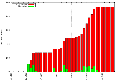
Figure 2: Monthly and cumulative distributions of observational epochs in the 19hr field as of 27th May 2010. There are seasons when observations were frequent with a handful of images taken every night and there are big gaps when the survey was not scheduled for observation.

The WTS has a lower priority than most of the main UKIRT programmes, thus observations are not distributed uniformly over time. For any given field, such as the 19 hour field (Fig. 2), there are large gaps when the field is not visible, as well as variations between and within seasons.

3 Pipeline overview

The WTS uses list-driven aperture photometry on processed images to construct lightcurves from the stacked data frames at the pawprint level. We describe this procedure briefly in this section.

3.1 2D pipeline

All images taken with WFCAM are processed using an image reduction pipeline operated by the Cambridge Astronomical Survey Unit (CASU). The WFCAM pipeline loosely evolved from strategies developed for optical processing (e.g. the Wide Field Survey on the Isaac Newton Telescope, (Irwin & Lewis, 2001)) and implements methods originally presented in Irwin (1985). The 2D processing is a fairly standardized procedure for the majority of projects using WFCAM on UKIRT. We give a brief overview of the image processing steps here.

Images are converted into multi extension FITS format, containing the data of the 4 detectors in one pawprint as extensions. Other data products from the pipeline (catalogues, lightcurves) are also stored in binary FITS table files. A series of instrumental correction steps is performed, accounting for: nonlinearities, reset-anomalies, dark current, flatfielding (pixel-to-pixel), defringing and sky subtraction. The sky subtraction removes any spatial variation in the sky background but preserves its mean level. The sky background is calculated as a robust $k\sigma$ clipped median for each bin in a coarse grid of 64x64 pixels. The sky background map is filtered by 2D bilinear and median filters to avoid the sky level shifting in bins dominated by bright objects. The final step is to stack the 9 individual WTS exposures to produce one 90 second exposure. Note that a simplified version of the catalogue generation and astrometric calibration steps (described below) are run on the individual unstacked exposures to ensure that they can be aligned before combining.

3.2 Catalogues, Astrometry and Photometry

Object detection, astrometry, photometry and classification are performed for each frame. Object detection follows methods outlined in Irwin (1985) (see also Lawrence et al. (2007)). Background-subtracted object fluxes are measured within a series of soft-edged apertures (i.e. pro-rata division of counts at pixels divided by the aperture edge). In the sequence of apertures, the area is doubled in each step. The scale size for these apertures is selected by defining a scale radius fixed at 1.0 arcsec for WFCAM. A 1.0 arcsec radius is equivalent to 2.5 pixels for WTS non-interleaved data. In 1 arcsec seeing an rcore-radius aperture contains roughly 2/3 of the total flux of stellar images. Morphological object classification and derived aperture corrections are based on analysis of the curve of growth of the object flux in the series of apertures (Irwin et al., 2004).

Astrometric and photometric calibrations are based on matching a set of catalogued objects with the 2MASS (Skrutskie et al., 2006) point source catalogue for every stacked pawprint. The astrometry of data frames are described by a cubic radial distortion factor (zenithal polynomial transformation) and a six coefficient linear transformation allowing for scale, rotation, shear and coordinate offset corrections. Header keywords in FITS files follow the system presented in Greisen & Calabretta (2002); Calabretta & Greisen (2002). The photometric calibration of WFCAM data is described in Hodgkin et al. (2009). These calibrations result in the addition of keywords to the catalogue and image headers, enabling the preservation of the data as counts in original pixels and apertures.

3.3 Master catalogues

Following the standard 2D image reduction procedures, catalogue generation and calibration, we have developed our own WTS lightcurve generation pipeline. This is largely based on previous work for the Monitor project described in Irwin et al. (2007) where more technical details are given.

As a first step in the lightcurve pipeline, master images are created for each pawprint by stacking the 20 best-seeing photometric frames. The master images play dual roles in our processing: they define the catalogue of objects of the survey for each pawprint with fixed coordinates and identifications numbers (IDs). Thus the source-IDs will never change for the WTS, however their coordinates could if we were to include a description of their proper motions. This has not yet been done.

Source detection and flux measurement is performed for each master image to create a series of master catalogues, and astrometric and photometric calibration recomputed, again with respect to 2MASS. These object positions are then fixed for the survey. Each source has significantly better signal-to-noise on the master image, and thus better astrometry (from reduced centroiding errors) than could be achieved in a single exposure. As discussed in Irwin et al. (2007), centroiding errors in the placement of apertures can be a significant source of error in aperture photometry, particularly for undersampled and/or faint sources.

This master catalogue is then used as an input list for flux-measurement on all the individual epochs, a technique we call list-driven photometry. A WCS transformation is computed between the master catalogue and each individual image using the WCS solutions stored in the FITS headers. Any residual errors in placing the apertures will typically be small systematic mapping errors that affect all stars in the same way or vary smoothly across frames. In practice, this can be corrected by the normalization procedure (see Section 3.4). The same soft-edged apertures are used (as described above), except that the position of the source is no longer a free parameter. Thus for each epoch of observation, a series of fluxes for the same sources is measured.

3.4 Lightcurve Construction and Normalization

Although the photometry of each frame is calibrated individually to 2MASS sources (Hodgkin et al., 2009), these values can be refined for better photometric accuracy. Lightcurves constructed using the default calibrations typically have an $RMS$ at the few percent level (for bright unsaturated stars). To improve upon this, an iterative normalization algorithm is used to correct for median magnitude offsets between frames, but also allowing for a smooth spatial variation in those offsets. In each iteration, lightcurves are constructed for all stellar objects and a set of bright stars selected ($13<J<17$) excluding the most variable decile of the group based on their (actual iteration) lightcurve RMS. Then for each frame, a polynomial fit is performed on the magnitude differences between the given frame magnitudes and the corresponding median (lightcurve) magnitude for the selected objects. The polynomial order is kept at 0 (constant) until the last iteration. In the last iteration, a second order, 2D polynomial is fitted as a function of image coordinates. For each frame, the best fit polynomial magnitude correction is applied for all objects and the loop starts again until there is no further improvement. Multiple iterations of the constant correction step help to separate inherently variable objects from non-variable ones initially hidden by lightcurve scatter caused by outlier frames. The smooth spatial component during the last iteration accounts for the effects of differential extinction, as well as possible residuals from variation in the point spread function (PSF) across the field of view.

It is also found that lightcurve variations correlate with seeing. In an additional post-processing step, for each object, a second order polynomial is fitted to differences from median magnitude as a function of measured seeing. Magnitude values are then corrected by this function on a per-star basis.

3.5 Bad epoch filtering

Data are taken in a wide range of observing conditions, sometimes with bad seeing ($\sim 2$ arcseconds or worse) or significant cloud cover. Additionally some frames are affected by loss and recovery of guiding or tip-tilt correction during the exposure. We identify and remove bad observational epochs that add outlier data points for a significant number of objects in any chip of a pawprint. Where a single (corrected) epoch has in excess of 30 per cent of objects deviating by more than $3\sigma$ from the median flux we flag and remove this epoch from all lightcurves. Fig. 3 shows some of the per-epoch parameters (which we store in the lightcurve files) as a function of $3\sigma$ outlier object ratio. The number of outlying objects has a strong correlation with the residual RMS of the second order polynomial normalization (panel a) which is a measure of the photometric unevenness of the image. The (cumulative) frame magnitude offset applied during the normalization (panel c) shows two distinct branches, and a large scatter can be seen in the average frame ellipticity (panel b). These two panels help to identify the main causes of bad epochs. High ellipticities arise from frames with tracking/slewing problems, while high magnitude corrections are suggestive of thick (and probably patchy) cloud. Our rejection threshold is a compromise between the number of affected frames and frame quality. At the outlier ratio threshold of 0.3, 39 frames (out of 950, or 4 per cent) are removed in the 19hr field.

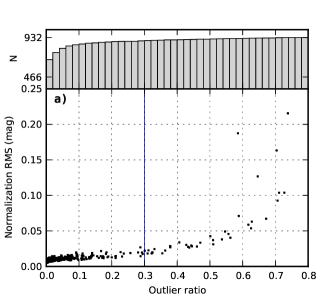
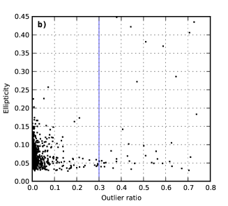
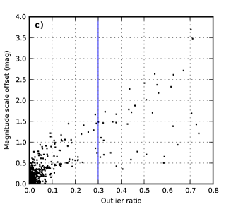
Figure 3: Per frame residual normalization RMS (a), average stellar ellipticity (b) and overall magnitude scale correction (c) as a function of $3\sigma$ outlier object ratio in the 19a pawprint. Epochs above a threshold of 0.3 are removed from the survey’s lightcurve release and candidate search. See text for more details.

3.6 Lightcurve quality

In Fig. 4 and Table 2 we summarize the WTS lightcurve quality at different pipeline steps. In each step we change or add one pipeline feature. The normalization procedure of the photometric scale by per-frame constant offsets (a), the quadratic spatial correction (b) during the normalization, the bad epoch filtering (c) and the seeing correction (d) give improvements at the several mmag level for unsaturated bright stars. In panel (d) a theoretical noise model curve consisting of Poisson noise, sky noise and a constant residual are drawn. A constant systematic error of 3 mmag is applied to the model shown in Fig. 4 to bring the model roughly into agreement with the data. This should be seen as the minimum systematic error in our lightcurves. Some saturation appears and makes lightcurve RMS worse for objects brighter than $J=13$ while for the faint end, the sky noise dominates.

$J=$	11-12	12-13	13-14	14-15	15-16	16-17
(a) constant normalization	9.3	6.1	5.7	6.6	9.7	19.1
(b) quadratic normalization	9.1	5.8	5.0	5.9	9.2	18.8
(c) + outlier filtering	8.7	5.6	4.9	5.7	8.8	18.1
(d) + seeing correction	7.3	4.8	4.6	5.6	8.5	17.6

Table 2: Median lightcurve RMS (mmag) as a function of object magnitudes using different pipeline options for the 19a pawprint. See text for details, and Fig. 4 for illustration.

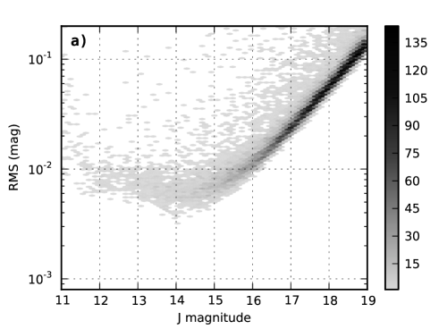
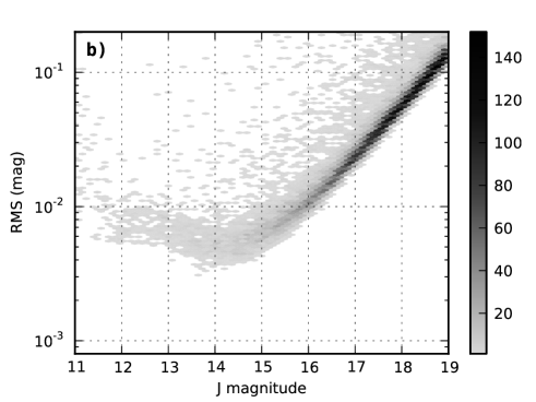
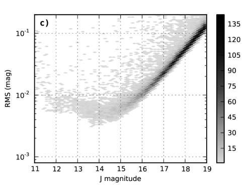
Figure 4: RMS of stellar objects in the 19a pawprint with different pipeline optimizations; a) constant normalization b) quadratic normalization c) outlier frame filtering d) seeing correction. In panel d) a noise model (thick red solid line) consisting of Poisson noise (dashed line), sky noise (dash-dotted line) and systematic noise of 3 mmag (thin blue solid line) is drawn.

3.7 Transit detection

To detect transit signals, we use a variant of the boxcar-fitting (Box Least Squares, or BLS) algorithm developed by Aigrain & Irwin (2004). They derive the transit fitting algorithm starting from a maximum likelihood approach of fitting generalized periodic step functions to the lightcurve. It was demonstrated that for planetary transits a simple box shaped function is sufficient. The algorithm in this form is equivalent to BLS developed by Kovács, Zucker & Mazeh (2002). The signal to red noise statistic is used to measure transit fitting significance (eq. 4 reproduced from Pont, Zucker & Queloz (2006)):

$$S_{\mathrm{red}}=\frac{d}{\sqrt{\frac{\sigma_{0}}{n}+\frac{1}{n^{2}}\sum_{i\not=j}C_{ij}}}$$ (1)

where $n$ is the number of in-transit data points in the whole lightcurve, $\sigma_{0}$ is the measurement error of the individual data points, $d$ is the fitted depth of the BLS algorithm, $C_{ij}$ is the covariance of two in-transit data points. Also following Pont, Zucker & Queloz (2006) we adopt a detection threshold of $S_{\mathrm{red}}=6$. Objects that pass this threshold are considered candidate transiting systems.

4 A sample of M dwarfs

4.1 Identification of M dwarfs

The high numbers of objects in the WTS and their faint magnitudes make spectral classification of all WTS objects potentially resource consuming. Instead, we use homogeneous broadband optical (from SDSS DR7, Abazajian et al. (2009)) and near-infrared (WFCAM) photometry to estimate reliable stellar spectral types. Specifically, effective temperatures are measured from fitting NextGen stellar evolution models (Baraffe et al., 1998) to $g$$r$$i$$z$ (SDSS) and $Z$$Y$$J$$H$$K$ (WFCAM) magnitudes. For comparison, we also fit the Dartmouth (Dotter et al., 2008) models, but in this case we use 7 passbands (Z and Y are not available). Least squares minimization is performed for the available photometry, fitting for temperature and a constant magnitude offset (distance modulus) as model parameters. The model grid data is smoothed by a cubic interpolation. We follow the temperature–spectral-class relation in Table 1 of Baraffe & Chabrier (1996): i.e. 3800K, 3400K, 2960K and 1800K corresponding to spectral types of M0, M2, M4 and M9 respectively.

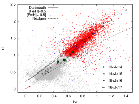
Figure 5: Colour-magnitude and colour-colour plots of the M dwarf sample ($13<J<17$, red crosses; $11<J<13$, blue crosses) of this study and other stellar objects ($10<J<16$) in the 19hr field based on WFCAM and SDSS data. A sequence of spectroscopic K and M dwarfs are shown from Covey et al. (2007) ($\square$) and Hewett et al. (2006) ($\circ$), respectively. Green markers show the M0 dwarf members of these sequences. Triangles ($\bigtriangledown$,$\bigtriangleup$) are M giants (III) from the same studies. Estimated maximum interstellar extinctions in different colours are marked by red arrows. Error crosses are from the corresponding catalogues.

Fig. 5 shows WFCAM and SDSS colour-magnitude and colour-colour panels of the stellar objects in the 19hr field. The M dwarf sample identified by the SED fitting on NextGen magnitudes is marked by red ($13<J<17$) and blue ($11<J<13$) crosses. A small number (6 per cent) of objects have outlying colour values due to saturation in one or more WFCAM or SDSS filters (typically $J<13$). These magnitudes are sigma-clipped during the SED fitting procedure. The panels also show 1 Gyr isochrones from the NextGen and Dartmouth models in the 2000K–6500K and 3200K–7700K temperature intervals respectively. The solid and dashed curves correspond to solar metallicity, the dash-dot to a metal-rich ([Fe/H]=+0.5), the dash-double-dot to a metal-poor ([Fe/H]=-0.5) model isochrone of the Dartmouth model respectively. Temperatures of 3800K and 3900K are marked (x) on the isochrones. Comparison between Dartmouth model isochrones show little significant difference in model colours between ages of 250Myr and 5Gyr. For very young stars, we might expect to pick up significant colour variation, however we expect very few very young (age $<100$ Myr) stars in our survey field. In fact Ciardi et al. (2011) analyse the very nearby Kepler field and find that the low-mass dwarf population is dominated by young thin disk stars, thus our selected age of 1Gyr is reasonable.

The figure also presents measured colours of K and M dwarfs and MIII giants of the Pickles photometric standards (dwarfs: $\square$, giants: $\bigtriangledown$) from Covey et al. (2007) and of the Bruzual-Persson-Gunn-Stryker atlas (dwarfs:$\circ$, giants:$\bigtriangleup$) from Hewett et al. (2006). All panels show colours in the Vega system, AB-Vega offsets are taken from Table 7 in Hewett et al. (2006), 2MASS-WFCAM conversions are calculated by relations given by Hodgkin et al. (2009). We denoted by filled green markers the M0 dwarf members (one and two objects, respectively) of these observations. Our identified M dwarfs are separated well from the sample of M giants ($\bigtriangledown$,$\bigtriangleup$) in the J-H vs. H-K and g-r vs. r-i panels, so we expect a low giant contamination level in our sample. The panels in Fig. 5 also demonstrate some difficulties in identifying M dwarfs. Model predictions do not reproduce observed patterns in all colour combinations. The NextGen isochrone has the best agreement in the infrared (J-H vs. H-K) while the Dartmouth models fit the r-i vs. i-z colours rather better. We note that the Nextgen colour predictions are too blue in the optical bands for low temperatures, which is a known model attribute (e.g. by 0.5 mag in V-I, Baraffe et al., 1998).

We also note that based on the residual $\chi^{2}$ values during the SED fitting procedure the photometric errors from the catalogues (shown in the colour-colour panels of Fig.5) were found to be underestimated. We assumed a systematic error between the WFCAM and SDSS catalogues and added a 0.03 mag systematic term in quadrature to the individual magnitude errors (used as weights in the fitting).

The Dartmouth data sets cover a narrower temperature range with a lowest temperature of 3200K. This makes the dataset unsuitable for selecting later (M4 and later) M dwarfs, although it gives a useful comparison for warmer stars. We conclude that for early M dwarfs (M0-2), the Dartmouth and Nextgen models give rise to very similar selections assuming solar metallicity. In the metal poor and metal rich cases the Dartmouth isochrones give about 40 per cent increase and 30 per cent decrease in numbers of early M dwarfs respectively.

In the g-r vs.  r-i diagram, we note that the scatter in g-r for objects with r-i$>1$ is larger (by about 0.2 mags at g=20) than can be explained solely from the SDSS photometric errors. This enhanced scatter can be explained by reddening alone (see below), and needs no significant spread in metallicity.

Leggett (1992) analyzed photometry of 322 M dwarfs and found that the effects of metallicity can be seen in M dwarf infrared colours (I-J, J-K, I-K, J-H, H-K) while not discernible in visible colours (U-B, V-I, B-V). They also noted that this feature is not reproduced by evolutionary models of Mould (1976); Allard (1990). We note that the Dartmouth model also shows a much smaller effect than seen in Leggett (1992) in the infrared, but a very large effect in g-r vs r-i.

In our paper, we base object classification on the NextGen model. Out of the 59000 morphologically identified stars in the $11<J<17$ magnitude range, we identified $\sim 4600$ M dwarfs. A more in-depth modelling of the objects in the WTS is an ongoing effort.

4.2 Interstellar extinction

During the SED fitting procedure, we cannot fit for the interstellar reddening and for the distance modulus on a per object basis due to being the fit badly determined. Therefore, we make an upper estimation for the reddening in our sample. We estimate a maximum distance for target M dwarfs of 1.5 kpc by assuming that one of our intrinsically brightest objects (an M0, M${}_{\rm J}=6$ from NextGen) is observed at the faint limit of the study ($J=17$). $A_{V}$ extinction values are calculated from the Galactic model of Drimmel, Cabrera-Lavers & López-Corredoira (2003). The three dimensional Galactic model consists of a dust disk, spiral arms mapped by HII regions and a local Orion-Cygnus arm segment. They use COBE/DIRBE far infrared observations to constrain the dust parameters in the model. We use the code provided to determine $A_{V}$ at 1.5 kpc. To calculate absorption in UKIRT and SDSS bandpasses, we use conversion factors $A/A_{V}$ from Table 6 of Schlegel, Finkbeiner & Davis (1998) that evaluates the reddening law of Cardelli, Clayton & Mathis (1989) and of O’Donnell (1994) for the infrared and the optical bands respectively. The reddening laws assume $R_{V}\equiv A_{V}/E_{B-V}=3.1$, an average value for the diffuse interstellar medium (Cardelli, Clayton & Mathis, 1989). Red arrows show our reddening estimates in different colours in Fig. 5 ($A_{V}:$ 0.409, $A_{J}$: 0.113, $E_{J-K}$: 0.067, $E_{J-H}$: 0.041, $E_{H-K}$: 0.026, $E_{g-r}$: 0.130, $E_{r-i}$: 0.083, $E_{i-z}$: 0.076). The total Galactic extinction in the 19hr field direction from Schlegel, Finkbeiner & Davis (1998) is $A_{V}=0.439$.

4.3 M dwarf bins

Stellar radius changes significantly between early- and late-type M dwarfs. For our sensitivity simulation purposes, we can use a linear approximation for the mass-radius relationship for M dwarfs: $M_{*}/M_{\mathrm{\odot}}\approx R_{*}/R_{\mathrm{\odot}}$. This slightly deviates from the NextGen mass-radius prediction (Baraffe et al., 1998) but it is in good agreement with observed M dwarf radii in Kraus et al. (2011). It is important in our simulations to treat early M dwarfs distinctly from later smaller M dwarfs. Therefore we divided our M dwarf sample into three coarse spectral bins. In the 19hr field, 2844 stars were identified as M0-2 ($3800\mathrm{K}>T_{\mathrm{eff}}>3400\mathrm{K}$), 1679 as M2-4 ($3400\mathrm{K}>T_{\mathrm{eff}}>2960\mathrm{K}$) and 104 as M4-9 ($2960\mathrm{K}>T_{\mathrm{eff}}>1800\mathrm{K}$). The third, latest (M4-9) type bin is very sparsely populated (2 per cent of the M dwarf sample) and numbers suffer from high uncertainty, so this bin will be omitted from the simulations, leaving us with two subsamples.

Considering the ‘colour distance’ along the isochrones between the boundary of our identified object groups, the Pickles M0 members (green squares) and the dependency of the isochrones on model parameters, we estimate the bin temperature edges to be uncertain about 250K.

4.4 M Dwarf Lightcurves

M dwarfs are known to be intrinsically more variable than more massive main sequence stars primarily due to spots (e.g.  Chabrier, Gallardo & Baraffe, 2007; Ciardi et al., 2011). The fraction of active M dwarfs also rises towards later (M4-9) subtypes (West et al., 2011). We examine the variability of the M dwarfs compared to the rest of the stellar sample in Table 3 and Fig. 6. The photometric precision is at the 4-5 mmag level for brighter objects ($J<15$) and at the percent level for the fainter region ($15<J<17$, 86 per cent of the M dwarfs). We compare the binned median RMS values of the three M subtypes to those of the warm (T$>$3800K) stars. Although the effect is small, we do find evidence that the median RMS for all three M dwarf samples is systematically higher, although only at about the 0.5-1 mmag level, at all magnitudes (see Fig.6).

We also calculate the fraction of $3\sigma$ outliers (a proxy for the most variable objects) for the different subsamples. We find that all three M dwarf samples, as well as the warmer stars exhibit a ten per cent outlier fraction.

Finally, these findings are also supported by 2D Kolmogorov-Smirnov tests (Fasano & Franceschini, 1987). The RMS versus magnitude distributions are found to be consistently different for each of the M dwarf samples versus the warm stars to very high confidence (test p values $<10^{-3}$). These results add support to the argument that observing in the J band gives limited sensitivity to spots (Goulding et al., 2012).

Typical signal depths for edge-on planetary systems are also shown in Fig. 6 to give a rough impression of our sensitivity. We expect to be able to detect Jupiter size planets in edge-on systems around all of our M dwarfs (in all spectral bins: M0-2, M2-4, M4-9), and Neptunes only in the M2-4 and M4-9 bins. As stated above, the latest type bin (M4-9) is sparsely populated, and omitted from the remaining analysis.

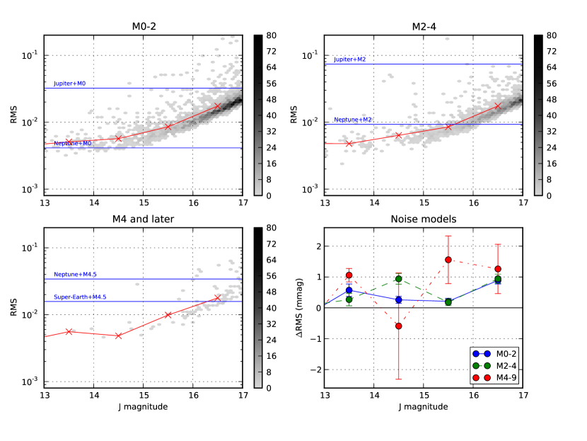
Figure 6: Comparison of lightcurve RMS in the M dwarf spectral groups. The solid curve shows median values of the RMS per magnitude bin. The bottom right panel shows the differences of the median RMS model curves from the median RMS of the earlier type stars. (M0-2: solid, M2-4: dashed, M4-9: dash dotted). Signal depths of edge-on transiting systems with Neptune, Jupiter or Super-Earth ($2.7R_{\oplus}$) size planets are marked.

$J=$	12-13	13-14	14-15	15-16	16-17
M0-2	4.4	5.1	5.7	8.5	17.4
M2-4	4.8	4.8	6.4	8.5	17.5
M4-9	3.9	5.6	4.8	9.9	17.8
Earlier types	4.8	4.5	5.4	8.3	16.6

Table 3: Median RMS (mmag) of M dwarf lightcurves and of earlier dwarfs for different object magnitudes.

4.5 The WTS sample compared to other surveys

The WTS is not the only transit survey specifically aimed at discovering planets around M dwarfs, and it is useful to place our survey in context. The MEarth survey individually targets about 2000 bright M dwarfs in a custom $i+z$-band filter (Berta et al., 2012). The survey was designed to focus on the nearest and brightest mid M dwarfs and has discovered one Super Earth size planet at the time of writing (Charbonneau et al., 2009).

The Palomar Transient Factory (PTF, Law et al. (2012)) is a project targeting M dwarfs in the R band. Their goal is to observe a total of 100,000 M dwarfs during the survey lifetime collecting about 300 epochs in each observing period. The PTF operates in roughly the same magnitude range (specifically over R=14–20) as the WTS and has a similar, seasonal observing schedule.

The Pan-Planets project also focuses on late-type stars. Their goal is to target approximately 100,000 M dwarfs in 40 square degrees. The programme collected about 100 hours of observations using the Panoramic Survey Telescope and Rapid Response System (PanSTARRS) so far (Koppenhoefer et al., 2009).

The Next-Generation Transit Survey (NGTS) is also an upcoming initiative to target a high number of bright M dwarfs ($V$<13) using wide field cameras. The prototype instrument observed $\sim$ 400 early and $\sim$ 50 late M dwarfs in 8 square degrees FOV at the one per cent photometric precision level (Chazelas et al., 2012).

Regarding space missions, the Kepler Mission in its Q2 data release has a relatively small (1086) number of M dwarfs but their data quality is much higher than for ground based programmes. The mission also samples uniformly in time with no large data gaps. We briefly discuss the planet occurrence rate in this sample in Section 7 based on H12 and compare it with our results.

Compared to these other transit surveys, the WTS is targeting a reasonable sample, even using only one of the four fields (at the time of writing three of the four fields are lagging in coverage). The PTF and Pan-Planets samples are potentially ground-breaking, if they can obtain enough observations.

4.6 A lack of hot Jupiters discovered around M dwarfs in the WTS

In the WTS, the initial candidate selection criterion is currently a well-defined decision based solely on the signal-to-noise ratio. Exhaustive eyeballing and photometric/spectroscopic follow-up of the small number of candidate planets around M dwarfs (Sipőcz et al., 2013) has revealed them all to be grazing eclipsing binary systems, or other false-positives. This search was complete for all $\sim$Jupiter-sized candidates down to J=17 in the 19 hour field, although avoiding objects with periods very close to one day. Two hot Jupiters have however been discovered around more massive hosts (Cappetta et al., 2012; Birkby et al., 2013). This confirms that the WTS is sensitive to transits at the $\sim 1$ per cent level (and indeed these two objects are very obvious). Zendejas et al. (2013) have independently produced lightcurves (using difference imaging) and searched for candidate planets in the same data, using stricter automated classification, and also find no candidate Jupiters around M dwarfs in the 19 hour field. This lack of hot Jupiters discovered around small stars in the WTS is what motivates the rest of this study, to address the question: how significant is this result.

5 Simulation method

5.1 Recovery ratio

We determine the sensitivity of the WTS for four distinct star-planet scenarios. For the two M dwarf subsamples, we consider Neptune and Jupiter size planets in short period (0.8–10 days) orbits around early (M0-2) and later type (M2-4) stars. The mass and radius of the star and the radius of the planet are kept fixed in each scenario (see Table 4). We use conservative assumptions for the stellar parameters: stellar radii are overestimated, using the maximum values in each spectral bin (i.e at M0 and M2), and planet radii are (under)estimated assuming solar system radii even for hot planets.

No.	Sp.bin	$T_{\mathrm{eff}}$ (K)	$M_{*}/M_{\mathrm{\odot}}$	$R_{*}/R_{\mathrm{\odot}}$	$M_{\mathrm{p}}/M_{\mathrm{Jup}}$	$R_{p}/R_{\mathrm{Jup}}$
1	M2-4	2960–3400	0.4	0.4	1.0	1.0
2	M2-4	2960–3400	0.4	0.4	0.054	0.36
3	M0-2	3400–3800	0.6	0.6	1.0	1.0
4	M0-2	3400–3800	0.6	0.6	0.054	0.36

Table 4: Simulated planetary systems

The expected number of recovered planetary systems can be written as:

$$N_{\mathrm{det}}=N_{\mathrm{stars}}fP_{\mathrm{det}}$$ (2)

where $N_{\mathrm{stars}}$ denotes the number of stars in the actual star subtype group, $f$ is the (unknown) fraction of the stars that harbour a planetary system, $P_{\mathrm{det}}$ is the (average) probability of discovering a system by the survey around one of its targets if we assume that the star harbours a (not necessarily transiting) planetary system. $P_{\mathrm{det}}$ is expressed as a function of planetary radius ($R_{p}$) and orbital period ($T$). In general, we can write (Hartman et al., 2009):

$$P_{\mathrm{det}}=\int\int P_{r}P_{T}p(R_{p},T)dR_{p}dT$$ (3)

where $P_{r}$ is the average recovery ratio, i.e. the average (conditional) probability of recovering a transit from a lightcurve if the lightcurve belongs to a transiting system, $P_{T}$ is the geometric probability of having a transit in a randomly oriented planetary system, and $p(R_{p},T)$ is the joint probability density function of $R_{p}$ and $T$ for planetary systems. We determine these terms in Eq. 3 separately in each scenario. See also Burke et al. (2006); Hartman et al. (2009).

We consider circular orbits only ($e$=0). $P_{T}$ can be given analytically, for a random system orientation, $P_{T}=(R_{*}+R_{p})/a$ where $a$ denotes the semi-major axis of the system, $R_{*}$ is the stellar radius. The joint probability density, $p(R_{p},T)$, must be treated as a prior. We consider planetary configurations at discrete $R_{\mathrm{P}}$ values only, so the $R_{\mathrm{P}}$ dependence of the density function simplifies to a $\delta$-function. As the period dependence is ill-constrained, we will discuss uniform and power-law functions as a prior distributions. In the H12 study, a power law model with an exponential cutoff at short periods was fitted (Table 5 in H12) to Kepler giant planet detections around mostly GK dwarfs (see sample criteria in Section 7). We use their model function normalized to our studied period range as prior distribution.

$P_{r}$ is determined numerically by the Monte Carlo iteration loop.

5.2 Determining $P_{r}$

We identify a set of 4700 quiet lightcurves in the 19hr field that serve as input for the simulations. This simulation sample consists of mostly M dwarfs (and slightly hotter stars) covering the magnitude range 11–17. The sample preserves the observed distribution of M dwarf apparent magnitudes in the WTS. By quiet we mean that the unperturbed lightcurves show no signature of a transit (BLS $S_{\rm red}<=6$). By adding noise free signals to these lightcurves and recovering them from the noisy data, we can quantify the effect of noise on $P_{r}$. As shown in Section 4.4, we found little difference between the noise properties of the lightcurves for the M0-2 and M2-4 subclasses. We simulate large numbers of transiting exoplanet systems to determine the recovery ratios for the four scenarios under investigation. In each iteration, a transiting planetary system is created with parameters randomly drawn from fixed prior distributions as detailed below (assuming a circular orbit). A simulated transit signal is then added to the randomly selected (real) lightcurve. We try to recover the artificial system using the transit detection algorithm discussed in Section 3.7 (Aigrain & Irwin (2004)). $P_{r}$ is estimated as the ratio between successful transit recoveries and the total number of iterations. We make a distinction between two different cases. In the threshold case we consider the signal successfully recovered if the detection passes the same signal to red noise level as used for WTS candidate selection ($S_{\mathrm{red}}$>6). In the periodmatch case, we additionally require that the recovered period value matches the simulated one. This is discussed in more detail in Sec. 6.3.

The period value ($T$) is drawn from a uniform distribution in the range of $0.8$ to $10$ days. The period determines the semi-major axis ($a$) of the system, given the masses of the star (assumed to be 0.6 or 0.4$M_{\odot}$) and the planet (assumed to be 1.0 or 0.054 $M_{\mathrm{Jup}}$). A randomly oriented system is uniformly distributed in $\cos i$ where $i$ is its orbital inclination. The random inclination is chosen to satisfy $0\leq\cos i<(R_{*}+R_{p})/a$ to yield a transiting system. This also allows for grazing orientations. The phase of the transit is also randomly chosen from within the orbital period.

Observed dates in the target lightcurve are now compared with predicted transit events. If there would be no affected observational epochs, then the iteration ends and the generated parameters recorded. Otherwise, a realistic, quadratic limb darkening model is used with coefficients from Claret (2000) to calculate brightness decrease at in-transit observational epochs (Mandel & Agol, 2002; Pál, 2008). This artificial signal is added to the lightcurve magnitude values, and BLS is run on the modified lightcurve. Both generated and detected transit parameters are recorded for the iteration. We note that the transit detection algorithm is the most computationally intensive step in the loop. A total of 75,000 iterations were performed.

6 Results and Discussion

6.1 Sensitivity effect of the observation strategy

The flexible observing mode of WTS has an inherent limitation on our sensitivity to short-period transiting systems, and it takes multiple seasons to build up enough epochs to reliably detect them. In Fig. 7 a simple sensitivity diagram is shown which considers only the actual distribution of observational epochs for the 19 hour field. We use the simulated transiting systems from the Neptune-size planets around an M0 dwarf scenario and compare the simulated transit times with our real observational epochs. A system is considered detectable here if at least 5, 10 or 15 in-transit observational epochs occur calculated from the simulated parameters. The fraction of detectable systems has an obvious strong dependence on the period of the transiting system and the required number of in-transit observational epochs as well. Of course, it depends on the noise properties of our data how many in-transit observations are necessary for detecting a transit event.

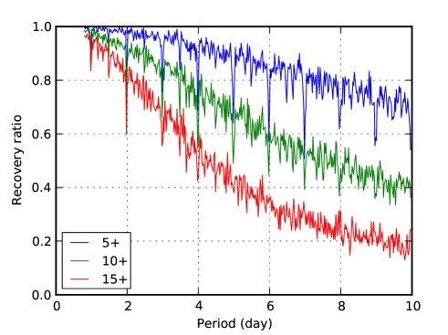
Figure 7: The effect of the observation strategy on the WTS sensitivity to short period transiting systems in the 19 hour field. We use the actual epochs of our 19 hour field observations combined with a large sample of simulated planets. The fraction of simulated transiting systems is shown where at least 5, 10 or 15 actual WTS observational epochs coincide with the simulated in-transit times. This illustration does not use the noise-properties of the WTS, thus does not consider the case as to whether the events are actually detected or not.

6.2 Detection statistic

We show the (signal to red-noise) detection statistic distributions in Fig. 8. The black curve belongs to the survey M dwarfs (unmodified data) in the 19hr field (selection criteria described in 4.3) . The coloured curves are for the simulated transiting systems for the four scenarios. For comparison, they are normalized to the total number of M dwarfs in the survey, i.e as if every WTS M dwarf target were either an M0 or an M2 with a transiting Jupiter or a Neptune (which may, or may not, have transited during the WTS observations).

The original (unperturbed) WTS M dwarf $S_{\mathrm{red}}$ distributions shows a marked tail above the detection threshold (25 per cent of all objects, see Sec.6.4). This could be caused by effects such as: correlated noise, intrinsic variability (spots), eclipsing binaries or possibly transiting planets. The simulations show that for initially “quiet” lightcurves ($S_{\mathrm{red}}<6$) the injection of a planet signal (transiting, but could be grazing) can perturb the measured signal-to-noise value above the detection threshold. (M2+J:50, M0+J:39, M2+N: 5.1, M0+N: 4.1 per cent of all iterations) In other words, the WTS is sensitive to Jupiters, and rather less sensitive to Neptunes. Given the other possible causes for a perturbed $S_{\mathrm{red}}$, the shape of this distribution does not in itself present a direct measurement of the planet population. It is worth noting that for the Jupiters (M0+J,M2+J), the recovered $S_{\mathrm{red}}$ values can be rather higher than the largest values we actually see in the WTS.

The Neptune cases have much smaller residual tails which sit only a little above the detection threshold. These signal injections cause detection statistic increases above the detection threshold only in a small number of cases. There is also little dependence on the size of the host star (the green and red curves are similar). Our simulations, with the same stellar magnitude distribution as the survey, are dominated by fainter objects. The similarity of the detection statistic distributions in the figure indicates that for Neptune sized planets, the survey sensitivity depends on the stellar radius only for the brightest stars. For fainter objects, the sensitivities are the same and as we see later, they are equally low (Figures 10 and 11).

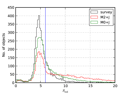
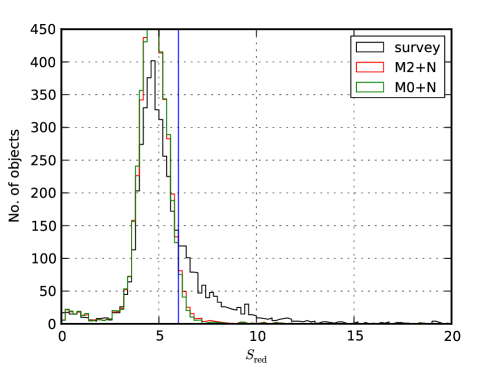
Figure 8: Detected signal to red noise histograms (bin size is 0.2) of the transit injected quiet lightcurve iterations (coloured) for Jupiter (left) and Neptune (right) size planets in the four simulated scenarios. For comparison, the unmodified (black) M dwarf lightcurves of the survey is shown and curves of the iteration loops are normalized to the number of M dwarf objects in the survey (black curve). The vertical line indicates our candidate selection threshold of 6.

6.3 Detected period

While passing the signal-to-noise statistic threshold in the simulation is caused by the injected signal, the detected (recovered) parameters, particularly the period, may not be correct. Indeed, it is common in ground based surveys to find multiple peaks in the BLS periodogram containing aliases of the observing window function.

The detected period is perhaps the most important of the model parameters: At the eyeballing stage of candidates, this period has the most influence in judging a transit detection real or false. In a lightcurve folded on the correct period (or a harmonic thereof), the transit signals are visually easily recognized. When folded on a random period, in-transit points are hardly distinguishable from random outliers. A good initial period value is also important for the timing of follow-up observations. With this in mind, we try to account for the importance of this effect in our simulations. We consider two recovery rates:

• threshold — $S_{\mathrm{red}}$ exceeds 6.0, and

• periodmatch — we additionally require that the detected period value matches (or be a harmonic of) the generated period. We allow factors of 1, 5/4, 4/3, 3/2, 5/3, 2, 5/2, 3, 4, 5 between the two values.

This step uses external information and obviously we cannot know the true period in the actual survey. However, in the simulations, it does allow us to place more strict criteria on detected simulated planets, and mimic the effects of differentiating between high priority candidates, which are likely to receive follow-up time, and low-priority candidates for which follow-up may be too expensive. This effect is much more significant for the Neptunes, where individual events are shallow.

We note that the number of in-transit data points is correlated with recovering the correct period. In the M2+J case, we find that if a simulated system has 10 in-transit data points we detect the correct period 80 per cent of the time, reaching almost 100 per cent with 20 in-transit data points. For larger stars (shallower transits), more in-transit data points are needed (M0+J: 12 and 30 points for 80 and 100 per cent respectively). For Neptunes even more transits are required to secure the period. For the M2+N case, we find 20 in-transit points recovers 50 per cent of the detected systems with the correct period. For the M0+N case the situation is even worse, and we almost always detect an alias (see Fig. 9). This confirms that the BLS algorithm is “lost” at these low signal levels. Comparing the necessary number of in-transit data points for reliable transit detections, according to Fig. 7, we can see an inherent limitation of the transit searching efficiency of the WTS and possibly other ground based low cadence surveys (e.g. PTF).

In this study we determine $P_{r}$ for the threshold and periodmatch cases. The real value of $P_{r}$ that characterizes the WTS probably lies between these two extremes and depends on all the (sometimes subjective) steps of the candidate selection and follow-up strategy. Having fewer quality criteria in the survey increase the number of candidates at the cost of higher false alarm ratio and more follow-up resource consumption.

We note that surveys with close to real time data processing and instant access to follow-up observation facilities could use a different approach and need not necessarily balance between quality of recovered transits and false positive rates. They can maximize the probability of detecting actual transit events by selecting follow-up times optimized to their current data and iteratively revise predictions as data accumulates. A Bayesian approach to such a strategy is described in Dzigan & Zucker (2011).

In Fig. 9 scatter diagrams and histograms of simulated and detected periods are shown for recovered simulated planets. We compare our most sensitive case in terms of injected signal depth (M2+J), to the least sensitive case (M0+N). They show a clear contrast in the quality of detected (signal to noise selected) transit signals.

For Jupiters, about 70 per cent of the detections also recover the injected period or its harmonic value (middle row in Fig. 9). Strong harmonic lines can be seen in the scatter panel (top left). For M0 stars (not shown), the ratio of recovered period values is even better. The shallower transits are longer in duration for a given period. The detected periods (bottom row, filled histogram) are biased towards shorter values peaking around 3 days, with aliases appearing at 1 and 2 days. In these iterations the injected signal changes the lightcurve in a way that aliased periods give the most significant box-fit signals. We see a gently decreasing trend for the periods of simulated systems that were recovered (bottom row, empty histogram), i.e. we are less sensitive to longer period planets, and more likely to underestimate their periods. We can conclude that signals of Jupiter sized planets can firmly be detected around all of the M dwarfs in the survey with good initial period values.

The Neptunes are shown in the right-hand column of Fig. 9. In accordance with our qualitative assessment based on the lightcurve RMS, signals of Neptune sized planets are at the boundary of being lost in the lightcurve noise in the WTS. In the M2+N case, only 12 per cent of the detections have also matching periods, in the M0+N case the correct period is almost never recovered by the box fitting algorithm (middle row). Recovered period values are heavily dominated by alias values. We conclude that Neptune sized planets can be detected in the survey only in favorable cases around smaller (later) M dwarfs.

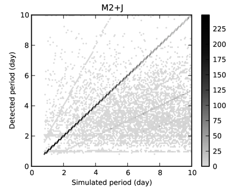
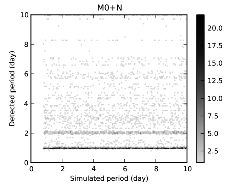
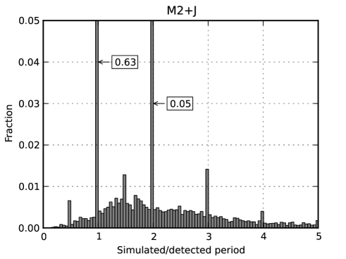
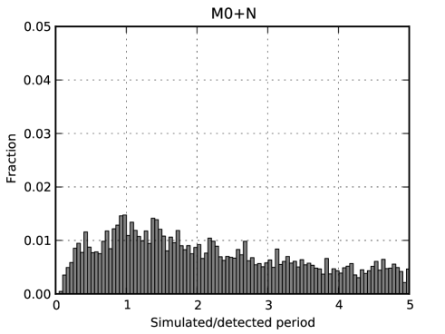
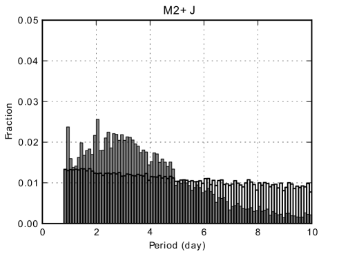
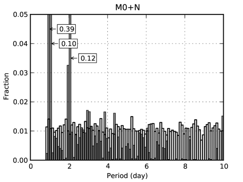
Figure 9: Properties of period values of iterations that pass the signal-to-noise threshold in the most (M2+Jupiter, left) and least (M0+Neptune, right) sensitive scenarios. Best fit detected period values as a function of simulated period values (top row) and normalized histograms of simulated/detected period ratios (middle row; bin size is 0.05). Bottom row: Normalized histograms (bin size 0.1) of detected (filled) and simulated periods (empty) i.e. projections to axes of top row scatter panels.

6.4 False positives

In a transiting planet survey, we have to deal with two types of false positives at the initial transit candidate discovery step. The detection statistic may pass where the transit box model is fitted just on (i) random fluctuations or systematics. In this case, the transit signal does not exist at all. (ii) Physical signals in the lightcurve may also belong to various eclipsing binary configurations or to variable stars (e.g. from spots) which can mimic transit events for the algorithm.

The amount of additional analysis to rule out false positive candidates can vary from little additional manual checking, through refinement of transit parameters, up-to obtaining additional observational data with better cadence. Grazing binary stellar systems can mimic planetary transits beyond the survey’s photometric precision and require additional spectroscopy measurements to be ruled out with high confidence.

The false positive ratio of the candidate selection procedure of the survey cannot be quantified by the simulation alone. A lightcurve passing the detection threshold with known injected simulated transit signal cannot be a false positive per se.

So far, all the actually selected, eyeballed and later followed-up (by additional photometry and/or spectroscopy) candidates around M dwarfs turned out not to be a planetary system (Sipőcz et al., 2013). Following Miller et al. (2008), this can be used to estimate the false positive ratio of the survey. This encompasses both false positive cases above. We assume that all $S_{\mathrm{red}}>6$ detections in our original (unmodified) lightcurves are false positives. At 25 per cent (black curve above the marker in Fig. 8), this is a rather large fraction. This number gives a simple (worst-case) description of our false positive ratio, and cannot be usefully applied to the simulations.

6.5 Transit recovery ratios

We show results of $P_{r}$ as a function of stellar magnitude for ranges of simulated period in Figs. 10 and 11. We adopt 0.8–3.0, 3.0–5.0, 5.0–10.0 day ranges following Hartman et al. (2009) for extremely hot Jupiters (EHJ), very hot Jupiters (VHJ), and hot Jupiters (HJ) respectively. Filled red circles (•) and green crosses (+) represent the threshold and periodmatch cases respectively. Integrated detection probabilities ($P_{\mathrm{det}}$) weighted by different prior assumptions including the geometric probabilities of transiting orientations are shown in Table 5.

For the Jupiter cases (upper rows in both figures), the WTS sensitivity has a maximum around J=13.5 and drops towards fainter (J>15-16) objects. This is in accordance with our expectations, we have higher noise levels towards fainter objects but there is occasional saturation at the bright end ($J<13$). There is little dependence on stellar radius, appearing only for the fainter stars. The threshold curves are less affected by simulated period than the periodmatch recovery rate. In the shortest period window the threshold and periodmatch values are practically the same. In the longest period panels the threshold ratio is about twice that of the periodmatch ratio showing that while the signal-to-noise detection statistic can recover signals, many of these systems may be missed due to poor initial period guesses. The survey has a much lower sensitivity for Neptunes (bottom rows in Figs. 10 and 11). The threshold curves show roughly 25 per cent of the recovery rate seen for Jupiters around bright stars. The difference between the threshold and periodmatch case is also more significant. The periodmatch recovery rates are close to zero for all M0 cases and very low for the M2 cases as well. The only exception is the best signal-to-noise case around M2 stars, in the short period window for bright objects where threshold rates reach half of the Jupiter value and the periodmatch rates are not close to zero. It looks like the WTS survey only really has a chance of discovering extremely hot Neptunes around late (M2 or later) and bright M stars ($J<15$). The lack of an accurate period determination would make follow-up of Neptune size candidates difficult in all other cases.

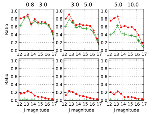
Figure 10: Recovery ratios ($P_{r}$) of simulated transiting system for M0+Jupiter (upper row) and M0+Neptune (lower row) scenarios in three period ranges as a function of stellar brightness. Filled circles (•) and crosses (+) represent the threshold and periodmatch ratio respectively.

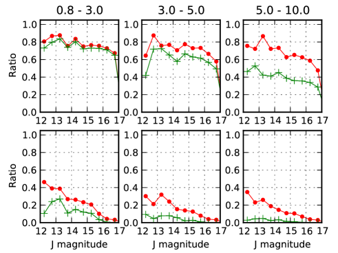
Figure 11: Recovery ratios ($P_{r}$) for M2+Jupiter (upper row) and M2+Neptune (lower row) simulated scenarios.

6.6 Error considerations

We use the seeing corrected lightcurves as a source for our simulation. While it could be more accurate to modify measured raw flux values and to run all the pipeline components to create the modified lightcurves, it would be unreasonably resource consuming, nor assumed to have an impact on our sensitivity results. Burke et al. (2006) decrease the sensitivity with a constant estimation of $0.03$ to deal with their trend filterings’ flattening effect. In our case it is assumed to have a negligible difference only as we do not use trend filters that uses solely lightcurve data. As it is described in the pipeline overview, images are transformed into lightcurves simultaneously, calculating magnitude scale offsets using non-variable, bright objects on each frame. Compared to the several thousand objects per frame, only a small fraction of objects may have a transit on a given frame thus the determined magnitude offset value would be independent of an injected signal. Being a bad weather fallback project, the survey typically has a few (2-3) observational epochs per observing night. Thus we do not expect significant correlation between the seeing and the timing of transit signals.

System type	prior	$N_{\mathrm{stars}}$	$P_{\mathrm{det}}$	$f_{\mathrm{95\%}}$	$P_{\mathrm{det}}$	$f_{\mathrm{95\%}}$
			sn	sn	pm	pm
M0+Jupiter	Kep.	2844	0.0363	2.9%	0.0311	3.4%
M2+Jupiter	Kep.	1679	0.0414	4.3%	0.0346	5.2%
M0-4+Jupiter	Kep.	4523	0.0382	1.7%	0.0324	2.0%
M0+Jupiter	uni.	2844	0.0360	2.9%	0.0305	3.5%
M2+Jupiter	uni.	1679	0.0405	4.4%	0.0332	5.4%
M0-4+Jupiter	uni.	4523	0.0377	1.8%	0.0315	2.1%
M0+Neptune	Kep.	2844	0.0027	39%	0.0001	100%
M2+Neptune	Kep.	1679	0.0025	71%	0.0003	100%

Table 5: Planet detection probability and upper limit results on planetary fractions in the WTS in the signal-to-noise threshold (sn) and periodmatch (pm) interpretation. The upper part shows limits for the simulated Jupiter scenarios (M0,M2) and its interpretation for the whole M0-4 dwarf sample. Values are shown for priors based on the H12 study (Kep.) and uniform (uni.). The lower part shows representative values for the Neptune cases.

6.7 Limits on planetary fraction

Assuming that the survey planetary candidates are all false positives, as our follow-up suggests (see Sec. 4.6), we can place upper limits on the planetary fraction ($f$) for our four test cases. The assumption of complete follow-up is much less secure for Neptune-sized planets, nevertheless the upper limits remain valid for the survey until a signal is detected. While Eq. 2 gives the expected number of detections, the actual number of detections follows a Poisson distribution. If the expected number of planets is $N_{\mathrm{det}}$, the probability of detecting $k$ planets is:

$$P_{k}=\frac{N_{\mathrm{det}}^{k}}{k!}\exp(-N_{\mathrm{det}})$$ (4)

We use this expression at $k=0$ as a likelihood function for $N_{\mathrm{det}}$. We require that $N_{\mathrm{det}}$ be within our $0\leq N_{\mathrm{det}}<N_{\mathrm{max}}$ confidence interval with 95 per cent confidence. Solving

$$P(N_{\mathrm{det}}<N_{\mathrm{max}})=\int\limits_{0}^{N_{\mathrm{max}}}\exp(-N)dN=0.95$$ (5)

for $N_{\mathrm{max}}$, we get $N_{\mathrm{max}}=3.0$. From the requirement of $N_{\mathrm{det}}<3.0$, using Eq. 2, we get:

$$f_{95\%}\leq\frac{3.0}{N_{\mathrm{stars}}P_{\mathrm{det}}}$$ (6)

Assuming zero detections and applying the above technique, we can compute robust upper limits on the fraction of planet host stars in our sample. We show the threshold and periodmatch $P_{\mathrm{det}}$ values along with the planetary fractions in Table 5. We show results for the two different assumptions for the period distribution: best fit exponential cut power law from Kepler (H12) (Kep.), uniform (uni.). For the hot Jupiters as a whole (periods 0.8–10 days), we can place an upper limit of $f_{95\%}=$2.9–3.4 per cent planet fraction around the early M subtype group (M0-2) assuming the Kepler power law prior period distribution. Using the simple uniform prior gives similar sensitivities (2.9–3.5 per cent) in this short period range. The smaller sample of cooler stars leads to a higher upper limit of 4.3–5.2 (4.4–5.4 for uniform) per cent for the M2-4 group. For Jupiter size planets, the threshold and periodmatch detection probabilities are essentially the same, and the chosen prior period distribution has also little impact.

We can combine the M0–M4 stars into one bin by calculating the average sensitivity for the whole sample weighted by the number of M dwarfs in the corresponding groups. The WTS can put an upper limit of $f_{95\%}=$1.7–2.0 (1.8–2.1 for uniform) per cent on the occurrence rate of short period Jupiters around early-mid (M0-4) M dwarfs. We discuss these results in context in Section 7.

For Neptunes, the WTS detection probabilities are an order-of-magnitude smaller than for Jupiters. We also find a strong dependence both on the assumed prior for the period distribution and the threshold/periodmatch interpretations. As seen, the recovery of Neptunes in the WTS is a difficult and unreliable task. The probability of recovering a Neptune with the correct period (periodmatch $P_{\mathrm{det}}$) is so low because detected signals are dominated by aliased periods. Thus it is very difficult to distinguish genuine Neptunes from false detections. The main way to improve on the WTS sensitivity to Neptunes would be to improve on the noise properties in the data. This is beyond the scope of this paper.

7 Discussion: Comparison with Kepler and RV studies

Although Kepler is not a specialized survey for M dwarfs, due to its exceptional quality data and large number of targets, it is probably the highest impact exoplanetary transit survey to date. In this section we compare our results to the planet occurrence study of the Kepler data in paper H12.

In the second part of the H12 study, the planet occurrence rate is determined in three planet radius bins (2-4$R_{\oplus}$, 4-8$R_{\oplus}$, 8-32$R_{\oplus}$) as a function of stellar type (effective temperature; in 500K wide temperature bins from 3600K to 7100K; see figure 8 in H12). They use the Q2 Kepler data release (Borucki et al., 2011). In each stellar temperature bin, the total planet occurrence rate is calculated by adding the contribution of each discovered (high quality) Kepler planet (candidate). eq.2 from H12 is reproduced here:

$$f=\sum_{j=1}^{N_{\mathrm{pl}}}\frac{1/P_{T}}{n_{*,j}}$$ (7)

$f$ is evaluated for each studied stellar bin. Each planet’s contribution is augmented by its geometric transit probability ($1/P_{T}$) to include planetary systems with non-transiting orientations as well (i.e. a detected planet with low geometric transit probability give a high contribution). Each planet’s fractional contribution is calculated over the number of high photometric quality stars only ($n_{*,j}$). Only those stars are selected from the Kepler Input Catalog (KIC) that belong to the analyzed stellar bin and have a high enough quality lightcurve where the actual planetary transit can be certainly detected (Table 6). A SNR value is derived from the edge-on planetary transit depth signal and from the measured scatter ($\sigma_{\mathrm{CDPP}}$; see eq.1 in H12) of the lightcurve. A lightcurve counts in the total number of stars if SNR>10 is fulfilled.

For transiting planets, a SNR>10 transit detection (calculated from the actual transit signal depth) and orbital period $T<50$ days are required. These planets are not all confirmed yet but part of the released Kepler planetary candidates passing an automated vetting procedure of the Kepler data processing pipeline. They are counted as planets both in H12 and in the present paper as they are assumed to be actual planets with high probability (Borucki et al., 2011).

Stellar effective temperature bins	3600–4100, …,
	6600–7100K
Stellar surface gravity, log g	4.0–4.9
Kepler magnitude, $K_{p}$	$<15$
Lightcurve quality, SNR	$>10$
Planetary radius bins, $R_{\oplus}$	2-4, 4-8, 8-32
Orbital period, $T$	$<50$ days
Detection threshold, SNR	$>10$

Table 6: Properties of stellar and planetary samples considered in the H12 Kepler study.

To obtain stellar parameters, the Kepler project uses model atmospheres from Castelli & Kurucz (2004). They perform a Bayesian model fitting on seven colours of the KIC objects determining effective temperature ($T_{\mathrm{eff}}$), surface gravity ($\log g$) and metallicity ($\log Z$) among other non-independent model parameters simultaneously (Brown et al., 2011). Restrictive priors also ensure that parameters remain within realistic value ranges. Temperatures are considered to be most reliable for Sun-like stars with differences from other models below 50K and up to 200K for stars further away from the Sun on the CMD. Brown et al. (2011) call temperatures below 3750K untrustworthy. There are 1086 M dwarfs identified in Q2 (Table 7).

Using the Q2 Kepler data release, we calculate Kepler planetary fractions for the 0.8–10 days period range to compare with our present WTS study. We follow the steps of H12 by selecting KIC objects and Kepler planets (candidates) from the Q2 data release using most criteria listed in Table 6 but selecting planets with $T<10\ \mathrm{days}$ (Fig. 12). We cannot filter for high quality lightcurves however as noise data is not readily available from H12. It is beyond the scope of this paper to process each released Kepler lightcurve and check its noise properties. Rather, we determine a correction factor for each stellar type bin. We reproduce the calculation for the planetary fraction in the $T<50$ day case omitting the lightcurve SNR>10 quality criterion and compare it to the published values in fig. 8 in H12. This reveals a correction factor that is applied to the $T<10\ \mathrm{day}$ case in each stellar bin (Table 7).

For stellar bins with nonzero planets 95 per cent confidence intervals (red error bars in Fig. 13) are calculated following the logic of ‘effective stars’ from H12; using a Poisson distribution for having the actual number of planet detections ($N_{\mathrm{pl}}$) from $N_{\mathrm{pl}}/f$ ‘effective stars’. Most stellar bins have only a few detections, so errors are heavily dominated by small number statistics. For bins with zero candidates (95 per cent confidence) statistical upper limits are calculated in the same way as for the WTS earlier in this study. In this case the number of ‘effective stars’ are calculated as the integrated overall detection probability in the 0.8–10 days period range.

In Fig. 13 and Table 7 Kepler planetary fractions ($f$) are shown for short period (0.8–10 days) hot Jupiters (8-32$R_{\oplus}$). E.g. in the coolest stellar bin, there are 9 planets (2-32$R_{\oplus}$) with period $T<50$ days, counting as 320.5 occurrences around 1086 M dwarfs. This yields a fraction of 0.295 which is the same rate published in H12. This means that the correction factor for the M dwarf bin (3600-4100K) is 1 i.e. all 1086 M dwarf lightcurves are good enough to detect planets down to super-Earth sizes. As there is no Jupiter size planet (8-32$R_{\oplus}$) in the 0.8–10 day period interval, we calculate an upper limit of the planet occurrence rate as $3/(1086\cdot 0.069)=0.04$.

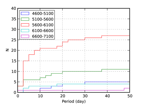
Figure 12: Cumulative number of discovered Jupiter size (8-32$R_{\oplus}$) planets in Kepler Q2 as a function of orbital period (T) in different stellar temperature bins. There are no planets in the two coolest stellar bins (3600–4100K, 4100K–4600K). Planet occurrence fractions in Fig. 13 are calculated for the 0.8–10 days region, augmenting the contribution of each discovery by its geometric transit probability.

Temp (K)	$N_{\mathrm{stars}}$	corr.	$N_{\mathrm{pl}}$	$N_{\mathrm{aug}}$	$f$	$f_{\mathrm{95\%}}$
3600–4100	1086	1.00	0	0		.04
4100–4600	1773	0.88	0	0		.027
4600–5100	6029	0.79	1	14.5	.003
5100–5600	18935	1.00	6	55.2	.003
5600–6100	31407	1.00	20	197.0	.006
6100–6600	11808	0.88	3	24.9	.002
6600–7100	2302	0.76	1	3.0	.002

Table 7: Total number of stars ($N_{\mathrm{stars}}$) in Kepler Q2 temperature bins, their corresponding correction (corr.) factors (see text), number of Jupiter size short period planets ($N_{\mathrm{pl}}$), their augmented contribution ($N\mathrm{aug}$) and the occurrence ratio ($f$) or upper limit ($f_{\mathrm{95\%}}$).

We recall that in this study 2844 early (M0-2, 3400K–3800K) and 1679 later type (M2-4, 2960K–3400K) M dwarfs were identified in the 19hr field of the WTS while there are 1086 early M dwarfs (3600K–4100K) in the Kepler Q2 dataset. Due to the factor of 2 higher number of early M dwarfs, the statistical upper limit set up by present study for the WTS M0-2 bin is a stricter constraint both in the threshold (2.9 per cent) and periodmatch approaches (3.4 per cent) than the one that can be derived for the (early) Kepler M dwarfs (4 per cent, Fig. 13). Though the WTS is more sensitive for Jupiters around later type M dwarfs, the upper limit for the M2-4 bin is slightly worse due to the smaller sample size: $f_{\mathrm{95\%}}=$4.3–5.2 per cent (depending on the period prior), while for the overall M0-4 sample, it is 1.7–2.0 per cent.

The WTS upper limits sit above the measured Hot Jupiter fractions found for hotter stars by Kepler which have much less uncertainty from much larger samples (bins with higher than 4600K in Fig. 13). With our analysis of the WTS, we cannot rule out a similar Hot Jupiter occurrence rate around M dwarfs (M0-4). Our main conclusion is that there is currently no evidence to support the argument that Hot Jupiters are less common around M dwarfs than around solar-type stars.

To push our constraints to lower levels we will need to complete the remaining three fields of the WTS, or wait for the completion of other surveys such as Pan-Planets (Koppenhoefer et al., 2009) or PTF (Law et al., 2012).

The completed WTS survey contains a total of almost 15,000 M0-4 dwarfs. A confirmed null detection for hot Jupiters in the larger sample would push our upper limit on the HJ fraction down by a factor 3.2, i.e. to $f_{\mathrm{95\%}}=$0.5–0.6 per cent for M0-4 stars. This will then overlap with the values found for hotter stars in Fig. 13.

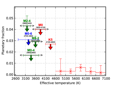
Figure 13: Short period (0.8–10 day) hot Jupiter planetary occurrence fractions (x) and upper limits ($\downarrow$) in case of null detections in the WTS (green), Kepler Q2 (H12) (red) and from the HARPS planet search (Bonfils et al., 2011) (blue). WTS upper limits are shown for the M0-2, M2-4 bins and also for the whole M0-4 sample (green arrows). Vertical error bars on WTS upper limit markers cover the uncertainty from the threshold and periodmatch interpretations (Table 5). Horizontal bars ($\vdash\dashv$) show temperature bin widths, horizontal arrows ($\leftrightarrow$) mark estimated uncertainty of bin edges where available. All upper limits and error bars of nonzero fractions are for 95 per cent confidence.

We note that the recent Kepler discovery and confirmation of KOI-254 (Johnson et al., 2012), a hot Jupiter planet around an M dwarf is beyond the parameter space considered in the H12 study thus cannot be directly incorporated into our comparison (object is fainter). Nevertheless, if this planet were part of the H12 sample, this sole detection would mean a $1.1_{-1.1}^{+4.1}$ per cent occurrence rate which is lower than the upper limits but still compatible with the findings of the present and the Bonfils et al. (2011) RV study. We note that this is an overestimation of the real weight of this planet detection as there are more cool hosts in KIC down to $K_{p}=$15.979 but linked to unknown, possibly lower survey sensitivity as well.

There are some caveats in our comparison. (i) The early M dwarf (M0-2) temperature bins are not exactly the same in the present WTS study (3400K–3800K) and in H12 (3600K–4100K) thus the WTS bins are apparently $\sim$ 250K cooler. However, we cannot use the same method to re-estimate temperatures for Kepler sources. Hopefully, as more follow-up data is released this will become possible. (ii) The sample of Kepler objects used to calculate planetary occurrences is restricted to bright objects ($K_{p}<15$) which is different from the magnitude range of WTS objects studied here ($J<17$). It is possible that the Kepler early M dwarf sample is from a different population than the sample in the present study (Mann et al., 2012). (iii) The sensitivity for Jupiters in the WTS was determined for a conservative $10R_{\oplus}$ radius while hot Jupiters may have larger radii. The Kepler study uses the 8–32$R_{\oplus}$ radius range for hot Jupiters.

7.1 Comparison with RV studies

Bonfils et al. (2011) analyze RV data observed by the ESO/HARPS spectrograph for planet signatures in their M dwarf (M0-6) sample of 102 nearby (<11pc, $V<14$) stars and find no Hot Jupiters. According to their sensitivity considerations, this sample is equivalent to 96.83 effective stars. Using our 95 per cent confidence level, their null detection of hot Jupiters (1-10 days) implies a 3.1 per cent upper limit on the planetary occurrence rate around M dwarfs, in good agreement with our WTS results.

Wright et al. (2012) find that 1.2$\pm 0.38$ per cent of nearby Solar-type stars host hot Jupiters. Their results are in good agreement with previous RV works (Marcy et al., 2005; Cumming et al., 2008; Mayor et al., 2011). Occurrence rates found by transit studies are systematically lower (Gould et al. (2006), H12), around 0.5 per cent.

As the rates around G dwarfs are about the same (RV) or lower (transit) than the upper limits reached by the WTS around M dwarfs in present study, we cannot rule out planet formation scenarios in this paper. We admit that this is a very brief comparison only, avoiding the discussion of the methods and error levels used by the studies cited above.

8 Summary

The WFCAM Transit Survey has observed 950 epochs for one of its four target fields. These data were collected over more than three years and will provide a valuable resource for general studies of the photometric and astrometric properties of large numbers of objects in the near-infrared. In this paper we determined the sensitivity of this dataset to short period ($<$10 day) Jupiter and Neptune sized planets around host stars of spectral type M0-M4. We identify and classify two subsamples of M dwarfs: M0-M2 comprising 2844 stars, and M2-M4 comprising 1679 stars. We compare Dartmouth and NextGen models to derive estimates of $T_{\mathrm{eff}}$ for the sample, and demonstrate that reddening effects are small for the 19-hour field. This forms one of the largest samples of M dwarfs targeted by any dedicated transit survey, and currently the only one working in the near-infrared.

We have described how our multi epoch WFCAM data are filtered and processed to produce lightcurves with median $RMS\sim 4$ mmag down to $J=14$ and $RMS\sim 17.5$ mmag at $J=17$. We found the $RMS$ for the brightest stars suffers a significant contribution from systematic noise at the $\geq 3$ mmag level. The origin of this is not determined, but we note that we see similar (albeit smaller) effects in the optical (e.g.  Irwin et al., 2007). We leave for future work an investigation of the flatfield and near-infrared background as two potential contributors to the systematics.

We performed Monte-Carlo simulations on the WTS lightcurves, injecting and recovering fake transit events. We generalise each of the stellar and planet populations into two distinct radius regimes, giving us 4 scenarios for transit depths: Jupiters and Neptunes, around M0-M2 stars and M2-M4 stars. We investigate the resultant signal-to-noise of the recovered events and compare this to the survey detection thresholds. We also investigate our sensitivity to these 4 scenarios as a function of orbital period and stellar magnitude. Our analysis of the simulations enables us to place constraints on the incidence of hot Jupiters.

With 95 per cent confidence and for periods $<$10 days, we showed that fewer than 4.3–5.2 per cent of M2-M4 dwarfs host hot Jupiters. Constraints are even stronger for earlier spectral types, and fewer than 2.9–3.4 per cent of M0-M2 dwarfs host hot Jupiters, while for the overall M0-4 sample, it is 1.7–2.0 per cent. An analysis of the Kepler Q2 data shows that the WTS provides more rigorous upper limits around cooler objects, thanks to the larger size of our sample (2844 M dwarfs in the WTS compared to 1086 in the Kepler sample under consideration). We compare these upper limits to the measured hot Jupiter fraction around more massive host stars, and find that they are consistent, i.e. we cannot rule out similar planet formation scenarios around at least the earlier M dwarfs (M0-4) at the moment.

We used our simulations to demonstrate that the WTS lightcurves are sensitive to transits induced by hot Neptunes in favorable cases, but that the ability to distinguish them from false alarms (astrophysical or systematic) is limited by a number of factors. Firstly the transit events have significantly lower to signal-to-noise than events arising from hot Jupiters, and thus the contamination by false alarms (from systematic noise) is higher at the required detection thresholds. Secondly, the recovered periods for the simulated hot Neptunes are dominated by spikes at multiples of 1 day, not seen so strongly for the larger planets. Without reliable periods, any attempts at follow-up photometry and spectroscopy for detected candidates will be hardly viable, especially for such faint target stars.

The data presented in this paper represent one quarter of the planned WFCAM Transit Survey (the other 3 fields currently lack sufficient coverage to include in the analysis). If the WTS is completed then we expect our statistical constraints to improve by a factor of 3–4 (dependent on the actual numbers of M dwarfs in the remaining three fields). If no hot Jupiters are found, our upper limits get to the 0.5 per cent level for M0-M4 dwarfs, and may ultimately reach a significantly lower level for hot Jupiter occurrence than is measured around G dwarfs by other surveys.

9 Acknowledgments

G.K. and B.S. are supported by RoPACS, a Marie Curie Initial Training Network funded by the European Commission’s Seventh Framework Programme. S.T.H. and D.P. are grateful to receive financial support from RoPACS during this research. The authors are thankful to S. Aigrain and J. Irwin for their algorithms and software development legacy from the Monitor project. This work also relies on image processing algorithms and implementations created by former and present members of the CASU group. The authors also thank M. Irwin for his useful comments on the paper.

References

- Abazajian et al. (2009) Abazajian K. N. et al., 2009, ApJS, 182, 543
- Aigrain & Irwin (2004) Aigrain S., Irwin M., 2004, MNRAS, 350, 331
- Allard (1990) Allard F., 1990, PhD thesis, PhD thesis. Ruprecht Karls Univ. Heidelberg, (1990)
- Baraffe & Chabrier (1996) Baraffe I., Chabrier G., 1996, ApJ, 461, L51
- Baraffe et al. (1998) Baraffe I., Chabrier G., Allard F., Hauschildt P. H., 1998, A&A, 337, 403
- Batista et al. (2011) Batista V. et al., 2011, A&A, 529, A102+
- Berta et al. (2012) Berta Z. K., Irwin J., Charbonneau D., Burke C. J., Falco E. E., 2012, AJ, 144, 145
- Birkby et al. (2013) Birkby J., et al., 2013, in prep.
- Bonfils et al. (2011) Bonfils X. et al., 2011, ArXiv e-prints
- Borucki et al. (2011) Borucki W. J. et al., 2011, ArXiv e-prints
- Borucki et al. (1997) Borucki W. J., Koch D. G., Dunham E. W., Jenkins J. M., 1997, in Astronomical Society of the Pacific Conference Series, Vol. 119, Planets Beyond the Solar System and the Next Generation of Space Missions, D. Soderblom, ed., p. 153
- Boss (2006) Boss A. P., 2006, ApJ, 643, 501
- Brown et al. (2011) Brown T. M., Latham D. W., Everett M. E., Esquerdo G. A., 2011, AJ, 142, 112
- Burke et al. (2006) Burke C. J., Gaudi B. S., DePoy D. L., Pogge R. W., 2006, AJ, 132, 210
- Calabretta & Greisen (2002) Calabretta M. R., Greisen E. W., 2002, A&A, 395, 1077
- Cappetta et al. (2012) Cappetta M. et al., 2012, ArXiv e-prints
- Cardelli, Clayton & Mathis (1989) Cardelli J. A., Clayton G. C., Mathis J. S., 1989, ApJ, 345, 245
- Castelli & Kurucz (2004) Castelli F., Kurucz R. L., 2004, ArXiv Astrophysics e-prints
- Chabrier (2003) Chabrier G., 2003, PASP, 115, 763
- Chabrier, Gallardo & Baraffe (2007) Chabrier G., Gallardo J., Baraffe I., 2007, A&A, 472, L17
- Charbonneau et al. (2009) Charbonneau D. et al., 2009, Nature, 462, 891
- Chazelas et al. (2012) Chazelas B. et al., 2012, in Society of Photo-Optical Instrumentation Engineers (SPIE) Conference Series, Vol. 8444, Society of Photo-Optical Instrumentation Engineers (SPIE) Conference Series
- Ciardi et al. (2011) Ciardi D. R. et al., 2011, AJ, 141, 108
- Claret (2000) Claret A., 2000, A&A, 363, 1081
- Covey et al. (2007) Covey K. R. et al., 2007, AJ, 134, 2398
- Cumming et al. (2008) Cumming A., Butler R. P., Marcy G. W., Vogt S. S., Wright J. T., Fischer D. A., 2008, PASP, 120, 531
- Dotter et al. (2008) Dotter A., Chaboyer B., Jevremović D., Kostov V., Baron E., Ferguson J. W., 2008, ApJS, 178, 89
- Drimmel, Cabrera-Lavers & López-Corredoira (2003) Drimmel R., Cabrera-Lavers A., López-Corredoira M., 2003, A&A, 409, 205
- Dzigan & Zucker (2011) Dzigan Y., Zucker S., 2011, MNRAS, 415, 2513
- Fasano & Franceschini (1987) Fasano G., Franceschini A., 1987, MNRAS, 225, 155
- Gillon et al. (2007) Gillon M. et al., 2007, A&A, 472, L13
- Gould et al. (2010) Gould A. et al., 2010, ApJ, 720, 1073
- Gould et al. (2006) Gould A., Dorsher S., Gaudi B. S., Udalski A., 2006, Acta Astron., 56, 1
- Goulding et al. (2012) Goulding N. T. et al., 2012, ArXiv e-prints
- Greisen & Calabretta (2002) Greisen E. W., Calabretta M. R., 2002, A&A, 395, 1061
- Hartman et al. (2009) Hartman J. D. et al., 2009, ApJ, 695, 336
- Hewett et al. (2006) Hewett P. C., Warren S. J., Leggett S. K., Hodgkin S. T., 2006, MNRAS, 367, 454
- Hodgkin et al. (2009) Hodgkin S. T., Irwin M. J., Hewett P. C., Warren S. J., 2009, MNRAS, 394, 675
- Howard et al. (2012) Howard A. W. et al., 2012, ApJS, 201, 15
- Ida & Lin (2005) Ida S., Lin D. N. C., 2005, ApJ, 626, 1045
- Ida & Lin (2008) Ida S., Lin D. N. C., 2008, ApJ, 685, 584
- Irwin et al. (2007) Irwin J., Irwin M., Aigrain S., Hodgkin S., Hebb L., Moraux E., 2007, MNRAS, 375, 1449
- Irwin & Lewis (2001) Irwin M., Lewis J., 2001, New A Rev., 45, 105
- Irwin (1985) Irwin M. J., 1985, MNRAS, 214, 575
- Irwin et al. (2004) Irwin M. J. et al., 2004, in Society of Photo-Optical Instrumentation Engineers (SPIE) Conference Series, Vol. 5493, Society of Photo-Optical Instrumentation Engineers (SPIE) Conference Series, Quinn P. J., Bridger A., eds., pp. 411–422
- Johnson et al. (2010) Johnson J. A., Aller K. M., Howard A. W., Crepp J. R., 2010, PASP, 122, 905
- Johnson et al. (2007) Johnson J. A., Butler R. P., Marcy G. W., Fischer D. A., Vogt S. S., Wright J. T., Peek K. M. G., 2007, ApJ, 670, 833
- Johnson et al. (2012) Johnson J. A. et al., 2012, AJ, 143, 111
- Kennedy & Kenyon (2008) Kennedy G. M., Kenyon S. J., 2008, ApJ, 673, 502
- Koppenhoefer et al. (2009) Koppenhoefer J., Afonso C., Saglia R. P., Henning T., 2009, A&A, 494, 707
- Kovács, Zucker & Mazeh (2002) Kovács G., Zucker S., Mazeh T., 2002, A&A, 391, 369
- Kraus et al. (2011) Kraus A. L., Tucker R. A., Thompson M. I., Craine E. R., Hillenbrand L. A., 2011, ApJ, 728, 48
- Laughlin, Bodenheimer & Adams (2004) Laughlin G., Bodenheimer P., Adams F. C., 2004, ApJ, 612, L73
- Law et al. (2012) Law N. M. et al., 2012, ApJ, 757, 133
- Lawrence et al. (2007) Lawrence A. et al., 2007, MNRAS, 379, 1599
- Leggett (1992) Leggett S. K., 1992, ApJS, 82, 351
- Mandel & Agol (2002) Mandel K., Agol E., 2002, ApJ, 580, L171
- Mann et al. (2012) Mann A. W., Gaidos E., Lépine S., Hilton E., 2012, ArXiv e-prints
- Marcy et al. (2005) Marcy G., Butler R. P., Fischer D., Vogt S., Wright J. T., Tinney C. G., Jones H. R. A., 2005, Progress of Theoretical Physics Supplement, 158, 24
- Mayor et al. (2011) Mayor M. et al., 2011, ArXiv e-prints
- Miller et al. (2008) Miller A. A., Irwin J., Aigrain S., Hodgkin S., Hebb L., 2008, MNRAS, 387, 349
- Mould (1976) Mould J. R., 1976, A&A, 48, 443
- O’Donnell (1994) O’Donnell J. E., 1994, ApJ, 422, 158
- Pál (2008) Pál A., 2008, MNRAS, 390, 281
- Pont, Zucker & Queloz (2006) Pont F., Zucker S., Queloz D., 2006, MNRAS, 373, 231
- Rodler et al. (2012) Rodler F., Deshpande R., Zapatero Osorio M. R., Martín E. L., Montgomery M. M., Del Burgo C., Creevey O. L., 2012, A&A, 538, A141
- Schlegel, Finkbeiner & Davis (1998) Schlegel D. J., Finkbeiner D. P., Davis M., 1998, ApJ, 500, 525
- Sipőcz et al. (2013) Sipőcz B., et al., 2013, in prep.
- Skrutskie et al. (2006) Skrutskie M. F. et al., 2006, AJ, 131, 1163
- Thommes, Matsumura & Rasio (2008) Thommes E. W., Matsumura S., Rasio F. A., 2008, Science, 321, 814
- West et al. (2011) West A. A. et al., 2011, AJ, 141, 97
- Wright et al. (2012) Wright J. T., Marcy G. W., Howard A. W., Johnson J. A., Morton T. D., Fischer D. A., 2012, ApJ, 753, 160
- Zendejas et al. (2013) Zendejas J., et al., 2013, in prep.