The Plateau de Bure + 30 m Arcsecond Whirlpool Survey
reveals a thick disk of diffuse molecular gas in the M51 galaxy

Abstract

We present the data of the Plateau de Bure Arcsecond Whirlpool Survey (PAWS), a high spatial and spectral resolution ¹²CO (1–0) line survey of the inner $\sim 10\times 6\,\mathrm{kpc}$ of the M51 system, and the first wide-field imaging of molecular gas in a star-forming spiral galaxy with resolution matched to the typical size of Giant Molecular Clouds (40$\,\mathrm{pc}$). We describe the observation, reduction, and combination of the Plateau de Bure Interferometer (PdBI) and IRAM-30m “short spacing” data. The final data cube attains $1.1\arcsec$-resolution over the $\sim 270\arcsec\times 170\arcsec$ field of view, with sensitivity to all spatial scales from the combination of PdBI and IRAM-30m data, and brightness sensitivity of $0.4\,\mathrm{K}$ ($1\sigma$) in each 5$\,\mathrm{km\,s^{-1}}$-wide channel map. We find a CO-luminosity of $9\times 10^{8}\,\mathrm{K\,km\,s^{-1}\,pc^{2}}$, corresponding to a molecular gas mass of $4\times 10^{9}\,\mathrm{M_{\odot}}$ for a standard CO-to-H₂ conversion factor. Unexpectedly, we find that a large fraction, $(50\pm 10)\%$, of this emission arises mostly from spatial scales larger than $36\arcsec\simeq 1.3\,\mathrm{kpc}$. Through a series of tests, we demonstrate that this extended emission does not result from a processing artifact. We discuss its origin in light of the stellar component, the $\mbox{${}^{12}$CO}/\mbox{${}^{13}$CO}$ ratio, and the difference between the kinematics and structure of the PdBI-only and hybrid synthesis (PdBI + IRAM-30m) images. The extended emission is consistent with a thick, diffuse disk of molecular gas with a typical scale height of $\sim 200\,\mathrm{pc}$, substructured in unresolved filaments which fills $\sim 0.1\%$ of the volume.

1. Introduction

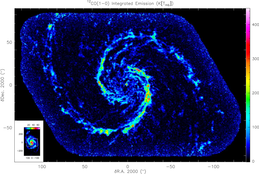
Figure 1.— ¹²CO (1–0) integrated emission of the inner $\sim 10\,\mathrm{kpc}\times 6\,\mathrm{kpc}$ of the galaxy NGC 5194 (M51a). The coordinate offsets are relative to the nucleus of NGC 5194 (see Table 1). This image results from the joint deconvolution of the IRAM-30m single-dish and Plateau de Bure interferometer data sets. The image inserted at the bottom left is the ¹²CO (1–0) integrated emission of the full M51 system (i.e., NGC 5194 + NGC 5195) as observed by the IRAM-30m telescope. The white horizontal rectangle shows the PAWS field of view. The images were scaled such that the angular resolution of both data sets occupies the same size on paper. In other words, the PAWS image shows the center of the small image zoomed by a factor of 21.

Table 1Parameters for NGC 5194.

Parameter	NGC 5194	Notes	Ref.
Morphological type	SA(s)bc pec		de Vaucouleurs et al. (1991)
Activity type	Seyfert 2		Véron-Cetty & Véron (2006)
Kinematic center	$13^{\mathrm{h}}29^{\mathrm{m}}52.7087^{\mathrm{s}};+47\arcdeg 11^{\prime}42.789^{\prime\prime}$	$\alpha,\delta$ J2000	Hagiwara (2007)
	$1.80^{\prime\prime},0.81^{\prime\prime}$	Offset from phase center
Distance	$7.6\pm 1\,\mathrm{Mpc}$	$1^{\prime\prime}=37\pm 5\,\mathrm{pc}$	Ciardullo et al. (2002)
Systemic velocity	$471.7\pm 0.3\,\mathrm{km\,s^{-1}}$	LSR, radio convention	Shetty et al. (2007)
Mean CO inclination	$21\pm 3\arcdeg$		Colombo et al. (2013b)
Mean position angle	$173\pm 3\arcdeg$		Colombo et al. (2013b)
Emitting surface	$1.9\times 10^{8}\,\mathrm{pc}^{2}$	$W_{\mathrm{CO}}\geq 3\sigma$	This work, Appendix A
Total CO luminositya	$1.4\times 10^{9}\,\mathrm{K\,km\,s^{-1}\,pc^{2}}$	in [LSR$-120$,LSR$+120$]$\,\mathrm{km\,s^{-1}}$	This work, Appendix A
Total molecular massa	$6.2\times 10^{9}\,\mathrm{M_{\odot}}$	Helium included	This work, Appendix A
Mean brightnessb	$7.6\,\mathrm{K\,km\,s^{-1}}$		This work, Appendix A
Mean mass surface densityb	$33\,\mathrm{M_{\odot}}\,\mathrm{pc}^{2}$		This work, Appendix A

^a Using the IRAM-30m data. ^b The mean brightness and mass surface density are computed using the area with significant emission, i.e., $W_{\mathrm{CO}}\geq 3\sigma$.

Along the path leading from the accretion of hot ionized gas onto galaxies to the birth of stars, the formation and evolution of Giant Molecular Clouds (GMCs) is the least well understood step. For example, the dependence of their mass distributions, lifetimes, and star formation efficiencies on galactic environment (e.g. arm, interarm, nuclear region) is largely unknown (for a review, see McKee & Ostriker, 2007). Because the Sun’s position within the Milky Way disk makes GMC studies difficult within our own Galaxy, observations of GMC populations in nearby face-on galaxies offer the best way to address many of these unknowns.

Complete CO maps that resolve individual GMCs have been carried out across the Local Group, allowing for the construction of mass functions and an estimation of GMC lifetimes via comparison with maps at other wavelengths (Kawamura et al., 2009). To date, these observations have probed mostly low mass galaxies where Hi dominates the interstellar medium (e.g., Blitz et al., 2007). The main reason is that the angular resolution required to identify individual GMCs (typical size $\sim$ 40$\,\mathrm{pc}$, e.g., Solomon et al., 1987) in any galaxy outside the Local Group is extremely difficult to achieve. Reaching such resolutions with single dish telescopes remains impossible in all but the very closest galaxies. This presents a major obstacle in linking our understanding of star formation and galactic evolution. Even for M31, the closest massive spiral galaxy to the Milky Way, the ¹²CO (1–0) IRAM-30m map achieves a spatial resolution of only 85$\,\mathrm{pc}$ and it suffers from projection effects (Nieten et al., 2006). This is an important problem because these massive star forming spirals dominate the mass and light budget of blue galaxies and they host most of the star formation in the present-day universe (e.g. Schiminovich et al., 2007).

To remedy this situation, we used the Plateau de Bure Interferometer (PdBI) to carry out the PdBI Arcsecond Whirlpool Survey (PAWS, Schinnerer et al., 2013). The high quality receivers and good weather conditions allowed PAWS to map the central, molecule-bright part of M51 at a resolution of $\sim 1.1^{\prime\prime}$ $(\sim 40\,\mathrm{pc})$ while still maintaining good brightness sensitivity (RMS $\sim 0.4\,\mathrm{K}$). M51 is the best target for such a program (see Table 1). It is one of the closest $(D\sim 7.6\,\mathrm{Mpc})$, face-on $(i\sim 21\arcdeg)$ grand design spirals, and it has been extensively studied at essentially all wavelengths. In contrast to Local Group galaxies with a resolved GMC population, the molecular gas clearly dominates the interstellar medium inside the mapped region (e.g., Garcia-Burillo et al., 1993; Aalto et al., 1999; Schuster et al., 2007; Hitschfeld et al., 2009; Leroy et al., 2009; Koda et al., 2011). M51 thus offers the opportunity to relate the physical properties of molecular gas to spiral structure. We complemented the interferometric data with a sensitive (RMS $\sim 16\,\mathrm{mK}$) map of the whole M51 system with the IRAM-30m single-dish telescope. This allowed us to produce a hybrid synthesis map — a joint deconvolution of the PdBI and IRAM-30m data sets — that is sensitive to all spatial scales between our synthesized beam and the PAWS field of view (see Fig. 1).

In Section 2, we detail the observing strategy and the data reduction. In Section 3, we show that a large portion ($\sim 50\%\pm 10\%$) of the emission in our hybrid maps arises from faint, extended structures. We provide a detailed discussion of the nature of the gas responsible for this emission. We summarize our conclusions in Sect. 4. The Appendices provide details on technical aspects of our observations, reductions and analysis, and additional supplementary Tables and Figures.

2. PAWS data acquisition and reduction

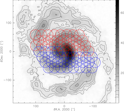
Figure 2.— Pointing pattern of the two observed PdBI mosaics overlaid on the integrated emission of the ¹²CO (1–0) line observed with the IRAM-30m. The 30 fields of each mosaic are displayed as red and blue circles, respectively. The diameter of each circle is $\lambda/d_{\mathrm{prim}}$, where $\lambda$ is the observation wavelength and $d_{\mathrm{prim}}$ is the diameter of an interferometer antenna, i.e., 15$\,\mathrm{m}$ for the PdBI. In our case, we have $\lambda/d_{\mathrm{prim}}\sim 36^{\prime\prime}$.

This section presents the observing strategy, the data reduction and the resulting data set. Sects. 2.1 and 2.2 focus on the PdBI and IRAM-30m data, respectively. Sect. 2.3 explains how we combined these data to produce a final set of hybrid maps sensitive to all spatial scales.

2.1. IRAM Plateau de Bure Interferometer data

After a discussion of the observing setup, we describe the calibration of the interferometric data.

2.1.1 Observations

PdBI observations dedicated to this project were carried out with either 5 or 6 antennas in the A, B, C, and D configurations (baseline lengths from 24$\,\mathrm{m}$ to 760$\,\mathrm{m}$) from August 2009 to March 2010. The two polarizations of the single-sideband receivers were tuned at 115.090$\,\mathrm{GHz}$, i.e., the ¹²CO (1–0) rest frequency redshifted to the LSR velocity (471.7$\,\mathrm{km\,s^{-1}}$) of M51. Four correlator bands of 160$\,\mathrm{MHz}$ per polarization were concatenated to cover a bandwidth of $\sim 550\,\mathrm{MHz}$ or $\sim 1430\,\mathrm{km\,s^{-1}}$ at a spectral resolution of $1.25\,\mathrm{MHz}$ or $3.25\,\mathrm{km\,s^{-1}}$.

We observed two 30-field mosaics, as described in Table 2 and shown in Fig. 2. Both mosaics were centered such that their combination covers the inner part of M51. The total field of view is approximately $270^{\prime\prime}\times 170^{\prime\prime}$. Each pointing was observed during $3\times 15$ seconds in turn. This allowed us 1) to observe one mosaic between two calibrations, which were taken every 22.5 minutes and 2) to minimize the dead-times due to moves from one field position to the next, while ensuring that the integration time per visibility (15 seconds) is short enough to avoid mixing independent $uv$ plane information in all the configurations (see, e.g., Appendix C.1 of Pety & Rodríguez-Fernández, 2010, for detailed calculations). An inconvenient aspect of such an observing strategy is that we obtained two data sets, observed in slightly different conditions, implying slightly different noise properties and $uv$ coverage (i.e. slightly different dirty/synthesized beams).

The field positions followed an hexagonal pattern, each field pointing being separated from its nearest neighbors by the primary beam full width at half maximum (FWHM), $\theta_{\mathrm{fwhm}}$. Nyquist sampling requires a distance between two consecutive pointings of $\lambda/d_{\mathrm{prim}}$ along two orthogonal axes, where $\lambda$ is the observation wavelength and $d_{\mathrm{prim}}$ is the diameter of the interferometer antennas. At PdBI, we typically have $\theta_{\mathrm{fwhm}}=1.2\lambda/d_{\mathrm{prim}}$. The hexagonal pattern used here thus ensures Nyquist sampling along the Declination axis but a slight undersampling along the Right Ascension axis.

The field-of-view was observed for about 169 hours of telescope time with 5 antennas in configuration D (19 hours) and 6 antennas in configuration C (18 hours), B (57 hours) and A (75 hours). Taking into account the time for calibration and the data filtering applied, this translated into final on–source integration times (computed for a 6-antenna array) of useful data of 8.3 hours in D configuration, 15.2 hours in C configuration, 43 hours in B configuration and 60 hours in A configuration. In each configuration, the time was approximately equally distributed between both mosaics.

2.1.2 Calibration

Table 2Parameters of the PdBI observations.

Molecule	Transition	Frequencies [$\,\mathrm{GHz}$]		Velocity [$\,\mathrm{km\,s^{-1}}$]
		Rest	Tuned	LSR	Tuned	Resolution
12CO	(1–0)	115.271202	115.090	471.7	0	5

Mosaic #	Projection center (J2000)		$N_{\mathrm{fields}}$	Beam	PA
	R.A	Dec.		${}^{\prime\prime}\times^{\prime\prime}$	$\deg$
Top	$13^{h}29^{m}54.921^{s}$	$47^{\circ}12^{\prime}21.589^{\prime\prime}$	30	$1.12\times 0.92$	61.5
Bottom	$13^{h}29^{m}50.504^{s}$	$47^{\circ}11^{\prime}03.642^{\prime\prime}$	30	$1.20\times 1.01$	84.0
Full	$13^{h}29^{m}52.532^{s}$	$47^{\circ}11^{\prime}41.982^{\prime\prime}$	60	$1.16\times 0.97$	73.0

Table 3Parameters of the 30m observations.

Molecule	Frequency	$F_{\mathrm{eff}}$	$B_{\mathrm{eff}}$	Resol.a	Resol.b	Map Size	Timec	$T_{\mathrm{sys}}$	$\sigma$
& Transition	GHz			$\,\mathrm{km\,s^{-1}}$	arcsec	arcmin2	hours	K [$T_{\mathrm{A}}^{*}$]	mK [$T_{\mathrm{mb}}$]
12CO (1–0)	115.271202	0.95	0.75	5.20/5.00	21.3/22.5	$53$ $(\sim 6\times 10)$	17.3/41	285	16
13CO (1–0)	110.201354	0.95	0.76	5.44/5.00	22.3/23.6	$53$ $(\sim 6\times 10)$	17.3/41	140	7.5

^a The two values correspond to the backend natural channel spacing and to the channel spacing used to match the PdBI channel spacing.
^b The two values correspond to the natural FWHM of the beam and to the map resolution after gridding through convolution with a Gaussian.
^c Two values are given for the integration time: the on-source time and the telescope time.

Table 4Median noise levels of the different ¹²CO (1–0) cubes.

Cube type	Resolution	$1\sigma$ Noise levels
	arcsec	($\,\mathrm{mK}$[$T_{\mathrm{mb}}$])	($\,\mathrm{K\,km\,s^{-1}}$)				$(\,\mathrm{M_{\odot}}\,\mathrm{pc}^{-2})$
			$5\,\mathrm{km\,s^{-1}}$	$25\,\mathrm{km\,s^{-1}}$	$50\,\mathrm{km\,s^{-1}}$	$100\,\mathrm{km\,s^{-1}}$	$5\,\mathrm{km\,s^{-1}}$	$25\,\mathrm{km\,s^{-1}}$	$50\,\mathrm{km\,s^{-1}}$	$100\,\mathrm{km\,s^{-1}}$
IRAM-30m	22.5	16	0.08	0.18	0.25	0.36	0.35	0.78	1.11	1.57
Hybrid synthesis	6.0	35	0.17	0.39	0.55	0.78	0.76	1.70	2.40	3.40
Hybrid synthesis	3.0	106	0.53	1.18	1.67	2.37	2.30	5.15	7.28	10.30
Hybrid synthesis	1.1	394	1.97	4.40	6.23	8.81	8.56	19.15	27.08	38.30
PdBI-only	6.0	38	0.19	0.43	0.60	0.85	0.83	1.85	2.62	3.71
PdBI-only	3.0	95	0.47	1.06	1.50	2.11	2.06	4.60	6.50	9.19
PdBI-only	1.1	396	1.98	4.43	6.27	8.86	8.62	19.26	27.24	38.53
Hybrid synthesis - PdBI-only	6.0	14	0.07	0.15	0.22	0.31	0.30	0.66	0.94	1.33
Hybrid synthesis - PdBI-only	3.0	25	0.12	0.27	0.39	0.55	0.53	1.19	1.69	2.39
Hybrid synthesis - PdBI-only	1.1	33	0.17	0.37	0.52	0.74	0.72	1.61	2.27	3.22

Standard calibration methods implemented inside the GILDAS/CLIC software were used for the PdBI data. The radio-frequency bandpass was calibrated using observations of two bright ($\sim$10 Jy) quasars, 0851$+$202 and 3C279, leading to an excellent bandpass accuracy (phase rms $\lesssim 1^{\circ}$, amplitude rms $\lesssim 1\%$). The temporal phase and amplitude gains were obtained from spline fits through regular measurements of the following close-by quasars: 1418$+$546, 1308$+$326, J1332$+$473. The flux scale was determined against the primary flux calibrator, MWC349. The resulting fluxes of the calibration quasars are summarized in Table 11. The absolute flux accuracy is $\sim$ 10%.

The data were filtered using statistical quality criteria on the pointing, flux, amplitude and phase calibrators. The source data were flagged when the surrounding calibrator measurements implied a phase rms larger than $40\arcdeg$, an amplitude loss larger than 22%, a pointing error larger than 30% of the primary beamwidth and/or a focus error larger than 30% of the wavelength. Finally, the data were also flagged when the tracking error was larger than 10% of the field of view. This reduces the amount of usable data to 39%, 70%, 71%, and 71% of the data obtained in the D, C, B, and A configurations, respectively.

2.2. IRAM-30m single-dish data

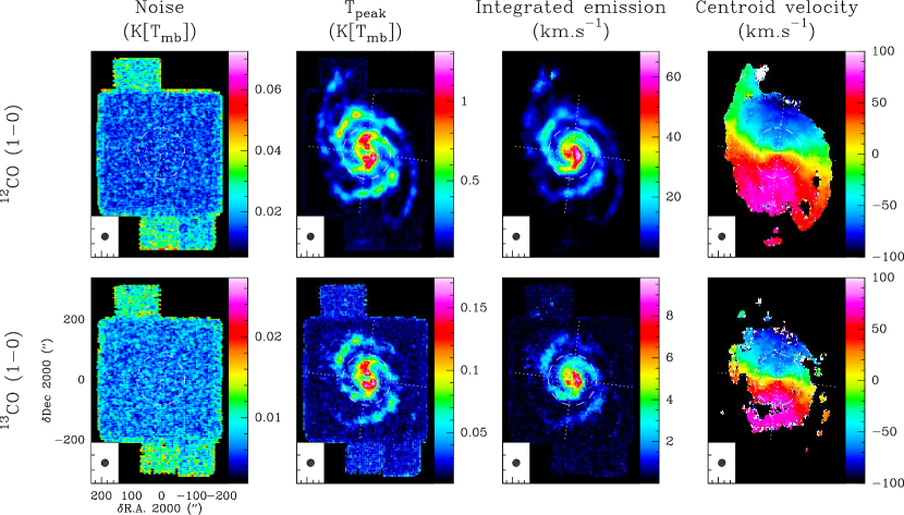
Figure 3.— Spatial distributions of the rms noise, peak intensity, integrated intensity and centroid velocity of the ¹²CO (upper panels) and ¹³CO (lower panels) (1–0) emission as observed with the IRAM-30m telescope. The angular resolution is displayed as a circle in the bottom left corner of each panel. The intensity scale is shown on the right side of each panel with units indicated in the caption title. The major and minor kinematic axes are displayed as perpendicular dotted lines. The dotted circles show the two inner corotation resonances at radii equal to $23^{\prime\prime}$ and $55^{\prime\prime}$, while the dashed circle marks the start of the material arms at a radius equal to $85^{\prime\prime}$ (Meidt et al., 2013).

A multiplicative interferometer filters out the low spatial frequencies, i.e., spatially extended emission. We thus observed M51 with the IRAM-30m single dish telescope on May 18-22, 2010 in order to recover the low spatial frequency (“short- and zero-spacing”) information filtered out by the PdBI. We describe here the observing strategy and the calibration, baselining and gridding methods we used to obtain single-dish data whose quality matches the interferometric data.

2.2.1 Observations

Table 3 summarizes the IRAM-30m observations. We used the EMIR receivers to map the ¹²CO (1–0) and ¹³CO (1–0) lines over a $\sim 60$ square arcminute field-of-view covering the M51 system, i.e., NGC 5194 and its companion NGC 5195. The upper sideband of the 3$\,\mathrm{mm}$ separated sideband EMIR mixers (E090) was tuned at the ¹²CO (1–0) frequency. The full 8 GHz bandwidth of the upper sideband was then connected to the WILMA autocorrelator backend. This allowed us to simultaneously measure the ¹²CO and ¹³CO lines (at 115.271 and 110.201$\,\mathrm{GHz}$, respectively). The backend channel spacing is 2$\,\mathrm{MHz}$, which translates into a velocity channel spacing of 5.4 and 5.2$\,\mathrm{km\,s^{-1}}$ at 110 and 115$\,\mathrm{GHz}$, respectively.

We observed the galaxy in seven different patches. Four of these covered the central $400^{\prime\prime}\times 400^{\prime\prime}$ part of the galaxy in different ways. Three additional patches extended the coverage to include the ends of the spiral arms and the companion. Conditions during the observations varied from “good” summer weather ($\sim 4\,\mathrm{mm}$ of precipitable water vapor) during the first three nights to “average” summer weather ($\sim 7\,\mathrm{mm}$ of water vapor) over the last two nights.

We used the position-switch on-the-fly observing mode, covering each field with back-and-forth scans along either the right ascension or declination axes. We slewed at a speed of $\approx 8^{\prime\prime}$/sec and we dumped data to disk every 0.5 seconds, yielding about 5.5 integrations per beam in the scanning direction (the HPBW of the IRAM-30m telescope at the frequency of the CO (1–0) line is $\sim 22^{\prime\prime}$). The scan legs were separated by $8^{\prime\prime}$, yielding Nyquist sampling transverse to the scan direction at 2.6$\,\mathrm{mm}$. Each position in the central part was observed 34 times on average, with observations split evenly between right ascension- and declination-oriented scanning to suppress scan artifacts. The sky positions at the far end of the CO spiral arms were observed 12 times so that the final effective integration time on the extensions is somewhat shorter than on the main field (see Fig. 3).

We observed the hot and cold loads plus the sky contribution every 12 minutes to establish the temperature scale and checked the pointing and focus every $\sim 1$ and $\sim 4$ hours. The IRAM-30m position accuracy is $\sim 2^{\prime\prime}$.

2.2.2 Calibration and gridding

We reduced the IRAM-30m data using a combination of the GILDAS software suite (Pety, 2005) and an IDL pipeline developed for the IRAM HERACLES Large Program (Leroy et al., 2009).

First, we calibrated the temperature scale of the data in GILDAS/MIRA based on the hot and cold loads plus sky observations (Penzias & Burrus, 1973). The resulting flux accuracy is better than 10% (Kramer et al., 2008). We then subtracted the “OFF” spectrum from each on-source spectrum. We used GILDAS/CLASS to write these calibrated, off-subtracted spectra to FITS tables which we read into IDL for further processing.

In IDL, visual inspection indicated the presence of signal in the $[-200,300\,\mathrm{km\,s^{-1}}]$ velocity range around the systemic velocity of the galaxy. About 1/16th of the 8$\,\mathrm{GHz}$ bandwidth (i.e. about 1000$\,\mathrm{km\,s^{-1}}$) centered on the line rest frequency were thus extracted from the calibrated spectra to reduce the computation load of the next data reduction steps. We then fit and subtracted a third-order baseline from each spectrum. When conducting these fits, we use an outlier-resistant approach and exclude regions of the spectrum that we know to contain bright emission based on previous reduction or other observations. We experimented with higher and lower order baselines and found a third-degree fit to yield the best results. After fitting, we compared the rms noise about the baseline fit in signal-free regions of each spectrum to the expected theoretical noise and used this to reject a few pathological spectra. For the most part the data are very well behaved and this is a minor step.

We gridded the calibrated, off-subtracted, baseline-subtracted spectra into a data cube whose pixel size is $4^{\prime\prime}$. Doing so, we weighted each spectrum by the inverse of the associated rms noise. We employed a gaussian convolution (gridding) kernel with FWHM $7.1^{\prime\prime}$, $\sim 1/3$ of the primary beam (e.g., see Mangum et al., 2007). This gridding increases the FWHM of the effective beam from $\sim 21.3^{\prime\prime}$ to $\sim 22.5^{\prime\prime}$ at 115$\,\mathrm{GHz}$.

After gridding, we fit a second set of third-order polynomial baselines to each line of sight through the cube. The process of the initial fitting and gridding is linear, so that these fits represent refinements to our initial fits after the averaging involved in gridding. We experimented with several more advanced processing options such as PLAITing (Emerson & Graeve, 1988) and flagging of standing waves. However the data were very clean and none of these algorithms improved the quality.

Figure 3 presents the reduced, calibrated, gridded IRAM-30m maps of the ¹²CO (1–0) and ¹³CO (1–0) line emission. The figure displays the spatial distributions of noise, peak temperature, integrated emission and centroid velocity. Fig. 26 and 27 (available in the electronic version only) display the channel maps of these lines.

2.3. Combination, imaging and deconvolution

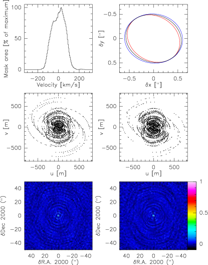
Figure 4.— Top, left: Area of the CLEAN mask, normalized to its maximum value, as a function of the channel velocity. Top, right: Ellipses representing the mean Gaussian beams for the top (red) and bottom (blue) mosaics. The black ellipse represents the Gaussian beam used for the restoration of the CLEAN component list. Middle: $uv$ coverages for the fields of the top (left panel) and bottom (right panel) mosaics. Bottom: Zoom of the dirty beams for the top (left panel) and bottom (right panel) mosaics.

The interferometric and single-dish data provide us with two data sets, which sample the high and low spatial frequencies, respectively. It is thus possible to produce two different deconvolved results: 1) one obtained from the interferometric data set alone, and 2) one obtained from the combination of the interferometric and single-dish data. While the latter is the desired final product, as it is sensitive to all measured spatial scales, the former is often produced because no single-dish measurements will be available or because they have not yet been acquired. In this paper, we will present both data cubes to emphasize the amount of flux which is recovered in the interferometric-only data set. Moreover, the angular resolution of the interferometric data is not uniquely defined. It depends on the weighting scheme chosen. For instance, it is sometimes useful to produce data cubes at lower angular resolutions to improve the brightness sensitivity, i.e., the sensitivity to extended emission. We exploit this here in addition to producing the full resolution cube.

This section explains 1) the generic imaging and deconvolution methods used to produce all these data cubes, 2) how these methods influence the amount of flux recovered in the interferometric-only data, and 3) the additional steps required to image jointly the single-dish and interferometric data.

2.3.1 Generic methods

Each interferometric pointing was imaged and a single dirty image was built by linear combination of the 60 individual dirty images. The dirty image was then deconvolved using an adaption of the Högbom CLEAN algorithm. A detailed account of the GILDAS/MAPPING implementation of the imaging and deconvolution processing of mosaics can be found in Pety & Rodríguez-Fernández (2010). To help the deconvolution, masks indicating the region where to search for CLEAN components were defined on individual channels from the short-spacing data cube. This cube was convolved with a Gaussian kernel to a final angular resolution of $30^{\prime\prime}$. The CLEAN masks were then defined by all the pixels whose signal-to-noise ratio was larger than 6. This method was designed to avoid biasing the deconvolution by defining masks wide enough to encompass all the detected signal from M51.

The deconvolution of each channel was stopped when a fraction of the maximum number of clean components were found. This fraction was defined as the ratio of the area of the current channel mask to the area of the wider channel mask (see left panel of Fig. 4). The deconvolution was assumed to have converged under three conditions. First, the cumulative flux as a function of the number of clean components converged in each channel. Second, the residual channel images looked like noise. Both criteria indicated a satisfying convergence of the deconvolution. Finally, we deconvolved again the data using exactly the same method except that we doubled the maximum number of clean components. The subtraction of both cubes looks like noise.

The list of clean components was regularized with a Gaussian beam and the residual image was added to obtain the final cube. As all the 30 fields of the top and bottom mosaics were regularly observed in short cycles of 22.5 minutes, the synthesized beams do not vary inside each mosaic. However, the two mosaics were observed at different times implying a slight difference of the synthesized beam between both mosaics (see Table 2). We used the same averaged Gaussian restoration beam for the northern and southern mosaic. This process is valid because 1) the Gaussian fits of the synthesized beams are similar as shown in the top right panel of Fig. 4 and 2) the remaining flux in the residual image is negligible or undetectable (i.e., below the noise limit). The resulting data cube was then scaled from Jy/beam to $T_{\mathrm{mb}}$ temperature scale using the restoration beam size.

While the natural velocity channel spacing of the interferometer backend is 3.25$\,\mathrm{km\,s^{-1}}$ at 2.6$\,\mathrm{mm}$, we smoothed the data to a velocity resolution of 5$\,\mathrm{km\,s^{-1}}$. This decreases the effect of correlation between adjacent frequency channels output by the correlator. This also increases the signal-to-noise ratio per channel (an important factor for the deconvolution) and speeds up the processing. Signal is present between $-110$ and $+110\,\mathrm{km\,s^{-1}}$, relative to NGC 5194’s LSR systemic velocity of 471.7$\,\mathrm{km\,s^{-1}}$. We thus imaged and deconvolved 120 channels producing a velocity range of $[-297.5,+297.5\,\mathrm{km\,s^{-1}}]$, implying that about two-thirds of the channels are devoid of signal. On a machine with 2 octa-core processors and 72 GB of total RAM memory, the deconvolution of the 120 channels up to a maximum number of 320 000 clean components typically took 38.5 hours (human time). The deconvolution duration increases linearly with the maximum number of clean components per channel.

2.3.2 PdBI only

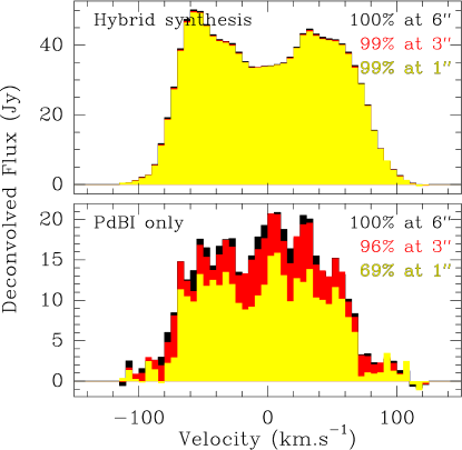
Figure 5.— Deconvolved flux as a function of velocity for the hybrid synthesis (top) and the PdBI only (bottom) data sets. Yellow, red, and black curves correspond to cubes imaged at an angular resolution of $1^{\prime\prime}$, $3^{\prime\prime}$, and $6^{\prime\prime}$, respectively. The percentage of total flux recovered compared to the $6^{\prime\prime}$ cube is indicated in the top right corner using the same color coding.

To start, we imaged and deconvolved the PdBI data without the short-spacings from the IRAM-30m observations. Achieving the convergence of the deconvolution algorithm at a given angular resolution is insufficient to prove that all the flux was recovered in PdBI-only data sets. Indeed, the absence of zero spacing implies that the total flux of the dirty image is zero valued, and it is the deconvolution algorithm which tries to recover the correct flux of the source. This works only when the source is small compared to the primary beam and the signal-to-noise is large enough. No deconvolution algorithm will succeed in recovering the exact flux of even a point source at low signal-to-noise. Indeed, the algorithm recovers only the flux which is above a few times the noise rms. Adding the deconvolution residuals will not help because the dirty beam (i.e., the interferometer response) has a zero valued integral, i.e., the residuals always contain zero flux.

Moreover, a given interferometer needs $2^{4}$ as much observing time to keep the same brightness sensitivity when just doubling the angular resolution (assuming similar observing conditions). Such an increase in observing time is impractical. The brightness sensitivity thus decreases quickly when the angular resolution improves. In the PAWS case, we approximately doubled the observing time every time we went to the next wider interferometer configuration, which typically doubled the angular resolution. This allowed us to reach a median noise of 0.4$\,\mathrm{K}$ at full resolution, i.e. $1.16^{\prime\prime}\times 0.97^{\prime\prime}$ at a position angle (PA) of 73 deg (when using natural weighting of the visibilities). While this is the best (pre-ALMA) sensivitivity reachable for such a large mosaic, it is also much higher than the sensitivity of 16$\,\mathrm{mK}$ we reached with the IRAM-30m at an angular resolution of $22.5^{\prime\prime}$. This may mean that faint intensities may be hidden in the noise of the $1^{\prime\prime}$-resolution cube.

Multi-resolution CLEAN algorithms (only available for single-field observations in GILDAS and thus not used for the PAWS mosaic) partly solve this problem of brightness signal-to-noise ratio because the deconvolution simultaneously happens on dirty images at different resolutions and thus different brightness noise levels. Interferometric brightness noise is a compromise between the synthesized angular resolution and the time spent in the different configurations. To check what happens with our deconvolution algorithm, we tapered the visibility weights to increase the brightness sensitivity at the cost of losing angular resolution, as this method is to first order similar to a Gaussian smoothing in the image plane. We choose Gaussian tapering functions such that we obtained synthesized resolutions of $3^{\prime\prime}$ and $6^{\prime\prime}$. Table 4 lists the typical rms noise values for the 3 different resolutions, i.e., 0.4, 0.1 and 0.03$\,\mathrm{K}$ at respectively $1^{\prime\prime}$, $3^{\prime\prime}$, and $6^{\prime\prime}$.

The lower panel of Fig. 5 visualizes the flux found by the CLEAN algorithm at the 3 different resolutions as a function of velocity. The Högbom CLEAN algorithm finds 40% more flux at $3^{\prime\prime}$ than at $1^{\prime\prime}$. On the other hand, only 4% more flux is recovered at $6^{\prime\prime}$ than at $3^{\prime\prime}$ even though the brightness sensitivity increases by a factor of $\sim 2.5$. Since the typical resolution of PdBI at 3$\,\mathrm{mm}$ in its most compact configuration is $6^{\prime\prime}$, it means that PdBI reaches its maximum brightness sensitivity in this configuration. Hence, further tapering the data would not recover more flux. Recovering only a marginal additional amount of flux when going from $3^{\prime\prime}$ to $6^{\prime\prime}$ thus implies that we recovered at these resolution all the flux present in the interferometric data.

2.3.3 Hybrid synthesis (PdBI + IRAM-30m)

The hybrid synthesis is a joint deconvolution of the PdBI and IRAM-30m data sets. The IRAM-30m and PdBI data sets were first made consistent using the following 4 steps. 1) We converted the IRAM-30m spectra to main beam temperatures ($T_{\mathrm{mb}}$) using the forward and main beam efficiencies ($F_{\mathrm{eff}}$ & $B_{\mathrm{eff}}$) given in Table 3. 2) These spectra were reprojected on the projection center used for the interferometric data set. 3) The LSR systemic velocity was set to zero to mimic observations at the redshifted frequency. 4) The velocity axis was resampled to 5$\,\mathrm{km\,s^{-1}}$ channel spacing. The last transformation introduced some correlation between channels as the autocorrelator natural channel spacing is only 5.2$\,\mathrm{km\,s^{-1}}$ at the ¹²CO (1–0) frequency.

Following Rodriguez-Fernandez et al. (2008), the GILDAS/MAPPING software and the single-dish map from the IRAM-30m were used to create the short-spacing visibilities not sampled by the Plateau de Bure interferometer. In short, the maps were deconvolved from the IRAM-30m beam in the Fourier plane before multiplication by the PdBI primary beam in the image plane. After a last Fourier transform, pseudo-visibilities were sampled between 0 and 15$\,\mathrm{m}$ (the diameter of the PdBI antenna). These visibilities were then merged with the interferometric observations. The relative weight of the single-dish versus interferometric data was computed in order to get a combined weight density in the $uv$ plane close to Gaussian. Since the Fourier transform of a Gaussian is a Gaussian, and the dirty beam is the Fourier transform of the weight density, this ensures that the dirty beam is as close as possible to a Gaussian, making this criterion optimum from the deconvolution point-of-view. In general, the short spacing frequencies are small compared to the largest spatial frequency measured by an interferometer. This implies we can use the linear approximation of a Gaussian in the vicinity of its maximum, i.e., one can assume the Gaussian is constant in the range of frequencies used for the processing of the short spacings. We thus need to match the single-dish and interferometric densities of weights in the inner region of the $uv$ plane.

In practice, we compute the density of weights from the single-dish in a $uv$ circle of radius $1.25d_{\mathrm{prim}}$ and we match it to the averaged density of weights from the interferometer in a $uv$ ring between 1.25 and $2.5d_{\mathrm{prim}}$. Experience shows that this gives the right order of magnitude for the relative weight and that a large range of relative weight around this value gives very similar final results (see e.g. Fig. 5 of Rodriguez-Fernandez et al., 2008). In our case, this computation was independently done for each interferometric pointing to take into account the fact that the two mosaics used to produce the final image were observed in slightly different conditions. The relative weight varies typically by 1% from pointing to pointing in each mosaic, and by $\sim 6-7\%$ between both mosaics.

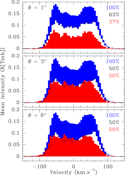
Figure 6.— Spectra, averaged over the field of view, of the hybrid synthesis (blue), PdBI-only (red) and filtered (= hybrid-PdBI, white) emission. The percentage of flux recovered in each spectrum is written in the top right corners with the same color code. The computations were done at the angular resolution displayed at the top left corner of each panel.

Contrary to interferometric-only data sets, the upper panel of Fig. 5 shows that the deconvolved flux in a hybrid synthesis is the same for the 3 different angular resolutions. In other words, the deconvolved flux is independent of the brightness sensitivity reached, as it is fully constrained by the zero spacing amplitude. Having high signal-to-noise zero spacing data thus ensures that the total flux inside the deconvolved cube will be the total flux of the single-dish data in the same field of view. Section 3.1.3 checks this for the PAWS data set. This is linked to the fact that the dirty beam integral is now normalized to unity. Both the dirty image and the residual fluxes are meaningful in this case. This enables an additional check of the convergence of the deconvolution algorithm for the hybrid synthesis deconvolution: We checked that less than 1.2% of the clean flux remains in the residual cube in the $[-100,+100]\,\mathrm{km\,s^{-1}}$ velocity range, even at $1^{\prime\prime}$ angular resolution.

Fig. 28 and 29 (available in the electronic version only) display the channel maps of the $1^{\prime\prime}$-resolution hybrid (30m+PdBI) synthesis cube at negative and positive velocities (relative to the systemic velocity), respectively.

3. A luminous component of extended emission

This section presents the unexpected finding that about half the CO luminosity in the hybrid map arises from a faint, extended component. Sect. 3.1 and 3.1.5 demonstrate that this result is unlikely to reflect an artifact in the data. Sect. 3.2 explores how the emission in the hybrid map breaks apart into a bright, compact and a faint, extended component. It also compares the structures of these distributions. Sect. 3.3 and 3.4 consider the nature of the CO emission components in light of 1) calculations of vertical disk structure, and 2) the observed ¹²CO/¹³CO ratio. Sect. 3.5 discusses our interpretation of this emission component.

3.1. Verifying the existence of an extended component

This section shows that $(50\pm 10)\%$ of the total flux in the PAWS field of view is filtered out by the interferometer. After a thorough discussion of several checks to prove that this is a true effect, we show that the filtered emission has typical spatial scales larger than $36^{\prime\prime}$, i.e., $1.3\,\mathrm{kpc}\,(D/7.6\,\mathrm{Mpc})$, where $D$ is the assumed distance of M51.

3.1.1 Flux recovered in the PdBI-only data cubes

Fig. 6 compares the spectra averaged over the field of view of 1) the hybrid synthesis data set (in blue) and 2) the PdBI-only data set (in red) for the 1, 3, and $6^{\prime\prime}$ data cubes from top to bottom. These spectra were obtained as a mean over the PAWS field of view contracted by about 1 primary beamwidth to decrease the influence of increasing noise at the map edges. The differences between the hybrid synthesis and PdBI-only spectra are displayed in white.

The main result is that only half of the total flux is recovered in the PdBI-only data set. Indeed, only 37% of the total flux is recovered at $1^{\prime\prime}$ but this is attributed to the relatively “low” brightness sensitivity reached at this resolution (see Section 2.3.2). Approximately 50% of the total flux is recovered both at $3^{\prime\prime}$ and $6^{\prime\prime}$, while the brightness sensitivity differs by a factor of 2.5 between them. We stress that although the deconvolution recovers 44% more flux at $6^{\prime\prime}$ than at $1^{\prime\prime}$, the difference amounts to only 13% of the total flux present in the PAWS field of view.

3.1.2 Coordinate registration

We checked the overall registration of the IRAM-30m moment-0 images against the PdBI-only data. We convolved these “reference” maps to the resolution of the IRAM-30m data. We then repeatedly shifted the images relative to one another and recorded the cross-correlation between the IRAM-30m data and the other images. The overall registration of the IRAM-30m with the PdBI data appears to agree within $\sim 1^{\prime\prime}$. In addition, we obtained the same agreement with the BIMA SoNG (Helfer et al., 2003) and CARMA (Koda et al., 2011) data. This good agreement is expected because radio-observatories check the coordinate registration directly against the radio-quasars used to define the equatorial coordinate frame.

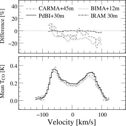
Figure 7.— Channel by channel flux comparison of the PdBI+30m, IRAM-30m, CARMA and BIMA data cubes over the PAWS field of view. The bottom panel shows the mean CO temperature as a function of the velocity and the top panel shows the relative difference with respect to the PdBI+30m data set. The dotted horizontal line indicates perfect agreement.

Table 5Comparison of registration and total flux within different ¹²CO (1–0) datasets.

Data set	Offset	Integrated flux	Flux difference
	arcsec	$10^{8}\,\mathrm{K\,km\,s^{-1}\,pc^{2}}$	% of PdBI+30m flux
IRAM-30m	$0$	7.82	$-0.5$
PdBI+30m	$<1$	7.86	$+0.0$
CARMA+45m	$<1$	7.41	$-5.7$
BIMA+12m	$<1$	7.03	$-10.6$

3.1.3 Flux calibration

As a test of our calibration strategy, we compared the flux within the hybrid synthesis data cube with recent CO surveys of M51 by BIMA (Helfer et al., 2003) and CARMA (Koda et al., 2011). Although conceptually straightforward, this comparison must be done with care since each dataset has different angular resolution, channel width, noise characteristics and field of view. To obtain the most meaningful comparison, we smoothed the BIMA, CARMA and hybrid synthesis data cubes to the same angular resolution as the IRAM-30m data $(22\farcs 5)$ and interpolated them onto a common $(l,m,v)$ grid with square pixels of $4^{\prime\prime}$ size, and a velocity channel spacing of 5$\,\mathrm{km\,s^{-1}}$. The grid uses a global sinusoid (GLS) projection, and is centered at RA 13:29:54.09, Dec $+$47:11:38.0 (J2000).

To define the region for the flux comparison, we constructed a mask of significant emission within the IRAM-30m data cube using the dilated mask technique described in Appendix B. In summary, this mask is obtained by the contiguous extension down to an intensity level of 2 times the rms noise $\sigma$ of all the pixels whose intensity is above $5\sigma$. The IRAM-30m $\sigma$’s were estimated for each sightline using the median absolute deviation. The resulting mask was applied to all four data cubes. The total integrated flux within a spatial region corresponding to the PAWS field of view contracted by $\sim 1$ primary beam width was then computed for each data set.

The results are listed in Table 5. The flux of the combined hybrid synthesis cube agrees with the flux of the IRAM-30m to within 1%, which is expected since the algorithm that we have used to combine the interferometer and single-dish data is designed to conserve flux. The integrated fluxes estimated from the PdBI+30m, CARMA+45m and BIMA+12m surveys agree to within 10%, which is the typical accuracy of the absolute flux calibration of radio observatories at millimeter wavelengths.

Figure 7 shows the global spectrum of the four surveys from the comparison region (bottom panel) and the relative flux difference per velocity channel between PAWS and the three other data sets (top panel). In general, the flux differences for individual velocity channels are consistent with the integrated measurements, i.e., there is $\sim$10% (5%) less flux in each channel of the BIMA+12m (CARMA+45m) data cube compared to PdBI+30m.

These tests confirm the IRAM-30m flux calibration accuracy and its correct transmission to the hybrid synthesis data set. As a test of the flux accuracy of the PdBI-only data set, we compared the efficiencies resulting from the interferometric flux calibration to the well-known PdBI antenna efficiencies as measured through regular holographies. These agree within $\sim 10\%$. The key point here is that the flux calibration is relatively straightforward at 3$\,\mathrm{mm}$, because the antennas have an excellent efficiency and the atmosphere was mostly transparent when the data was acquired (as confirmed by the achieved system temperatures listed in Table 10).

3.1.4 Amplitude of the brightness Fourier transform as a function of the $uv$ distance

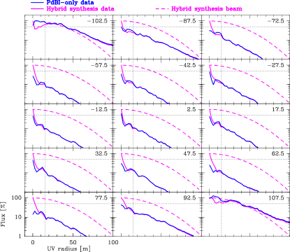
Figure 8.— Variations of the azimuthal average of the Fourier transform amplitude as a function of $uv$ radius for every third velocity channel between $-102.5$ and $+107.5\,\mathrm{km\,s^{-1}}$. On the y-axis, we plot the percentage of the maximum flux at the zero $uv$ radius. The pink dashed curve displays the theoretical shape for a signal-free channel, i.e., the Fourier Transform of the hybrid synthesis beam. The pink and blue solid curves show, respectively, the hybrid synthesis and PdBI-only data imaged at $6^{\prime\prime}$ resolution. The dotted vertical line indicates the minimum $uv$ radius measured by the interferometer (i.e. $\sim 15\,\mathrm{m}$). The dotted horizontal line represents a 50% reduction in flux.

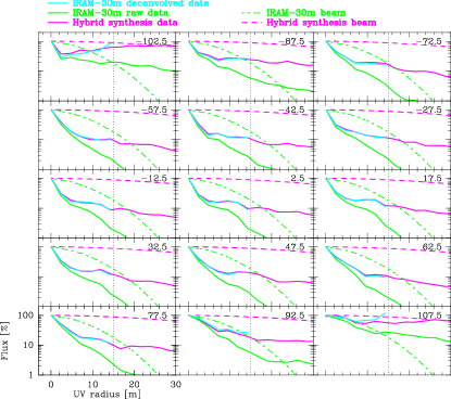
Figure 9.— Zoom of the variations of the azimuthal average of the Fourier transform amplitude as a function of $uv$ radius for every third velocity channel between $-102.5$ and $+107.5\,\mathrm{km\,s^{-1}}$. The y-axis shows the percentage of the maximum flux at zero $uv$ radius. The dashed pink and green curves display the Fourier Transforms of the hybrid synthesis and the IRAM-30m beams, respectively. The solid pink curve shows the hybrid synthesis data imaged at $6^{\prime\prime}$ resolution. The solid green and cyan curves represent, respectively, the IRAM-30m data before and after deconvolution from the $22.5^{\prime\prime}$ 30m beam and convolution with a $6^{\prime\prime}$ beam. The dashed vertical line indicates the minimum $uv$ radius measured by the interferometer (i.e., $\sim 15\,\mathrm{m}$).

It is important to test how well the hybrid synthesis and the PdBI-only data cubes agree with each other at high spatial frequencies. To do this, Fig. 8 compares the azimuthal average of the amplitude of the Fourier transform of the PdBI-only and the hybrid synthesis data cubes at $6^{\prime\prime}$ resolution as a function of the $uv$ distance for every third velocity channel between $[-102.5,+107.5]\,\mathrm{km\,s^{-1}}$. In such a representation, the amplitude at the zero $uv$ radius is equal to the total flux present in the channel map. We thus normalized all the curves inside each panel so that their zero-spacing values represent the fraction of the total flux available in the hybrid synthesis cube at this velocity channel. For reference, 1) the power spectrum would be computed as the square of these curves, 2) the dashed vertical lines indicate the minimum radius directly measured by the interferometer, i.e., $r_{\mathrm{min}}\simeq 15.1\,\mathrm{m}$. Moreover, noise and signal behave differently after undergoing a Fourier transformation. Noise (e.g., signal-free channels at the edges of the velocity range in the figure) will give a shape consistent with the Fourier transform of the Gaussian restoration beam (see Chapter 17 of Bracewell, 2000). On the other hand, signal channels display the product of Fourier transform of the true source brightness and the Fourier transform of the Gaussian restoration beam as a function of the $uv$ spacing. Hence, channels with significant line signal fall more quickly than the Gaussian restoration beam.

The good agreement between the amplitudes from the hybrid and PdBI-only data at radii larger than $r_{\mathrm{min}}$ provides confidence in the deconvolution results of the compact sources (whose angular extent is smaller than $\lambda/r_{\mathrm{min}}\sim 35^{\prime\prime}$) in the PdBI-only data set even though the short-spacings are missing. Below $r_{\mathrm{min}}$, the two curves diverge because the deconvolution can only “extrapolate” up to the zero $uv$ radius for the PdBI-only data set, while it “interpolates” for the hybrid synthesis data set. As the amplitude at zero spacing is proportional to the total flux, these plots clearly indicate that PdBI-only data miss a large fraction of the flux even for the $6^{\prime\prime}$ resolution cube, whose deconvolution is immune to low signal-to-noise effects.

Moreover, the change of slope visible in Fig. 8 for the hybrid synthesis amplitude between $\sim$ 5 and 15$\,\mathrm{m}$ is not a processing artifact. Indeed, Fig. 9 displays a zoom of the azimuthal average of the amplitude of the Fourier Transform of the IRAM-30m and the hybrid synthesis data cubes at $22.5^{\prime\prime}$ and $6^{\prime\prime}$ resolution (green and pink curves, respectively). These curves cannot be directly compared because they result from two different measurement equations (the single-dish and the interferometric ones). The solution is well-known: We just have to apply to the IRAM-30m curve the standard processing steps needed to produce short-spacing visibilities (see Sect. 2.3.3). Indeed, after deconvolution of the single-dish brightness by the $22.5^{\prime\prime}$ single-dish beam and multiplication with the $6^{\prime\prime}$ interferometric primary beam, the amplitudes of the Fourier transform of both data sets agree well. Since a Gaussian of $22.5^{\prime\prime}$ FWHM has a flux equal to 77, 45, and 21% of its maximum at 5, 10, and 15$\,\mathrm{m}$, the observed change of slope of the deconvolved 30m data cannot be attributed to imprecision in the deconvolution of the IRAM-30m beam. This change of slope in flux is responsible for the failure of the deconvolution to extrapolate the correct total flux at the zero $uv$ radius for the PdBI-only data set.

3.1.5 Impact of the IRAM-30m error beam

The beam efficiency of the IRAM-30m telescope at the frequency of the ¹²CO (1–0) line is predicted to be 0.78, based on the interpolation of the measured efficiencies at 86, 145, 210, 260, and 340$\,\mathrm{GHz}$ using the Ruze formula. Moreover, the forward efficiency is 0.95 at the same frequency. This implies that about 22% of the measured flux in a given direction results from beam pick-up from solid angles outside the main beam. Of this amount, 5% originates from the rear lobes, which mainly collects diffuse emission from the telescope backside. Hence, about 17% of the measured flux is picked up by the rings of the telescope diffraction pattern and the error beams due to the limited surface accuracy of the telescope. In Appendix C, we assess in-depth how much these effects contribute to the extended emission. Here, we summarize the main results.

We estimate that the peak brightness due to the error beam contribution is at most 55$\,\mathrm{mK}$, i.e., about 3.5 times the median noise level of the IRAM-30m observations. The median value of the error beam contribution is 19$\,\mathrm{mK}$, while pixels brighter than 5 times the noise level have a median of 140$\,\mathrm{mK}$ in the extended emission measured at $6^{\prime\prime}$ (see Sect. 3.2.1). The emission associated with the error beams has a very different signature from that of extended emission both in space and velocity. In particular, the putative error beam contribution translates into much wider lines than actually observed. Moreover, the typical angular scales of the error beams are large, implying that the flux is scattered at low brightness level over wide regions of the sky. Finally, we estimate that at most 10% of the total flux in the PAWS field of view can be due to error beam scattering.

Taken together, these arguments lead us to the conclusion that the IRAM-30m error beam cannot explain the presence and properties of the extended emission.

3.1.6 About half the CO luminosity arises from an extended emission component

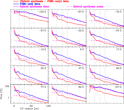
Figure 10.— Same as Fig. 8 but the pink dot-dashed curve displays the average noise level as a function of the $uv$ radius. The red curve shows the difference between the hybrid synthesis and the PdBI-only at $6^{\prime\prime}$ resolution. The 3 dotted vertical lines indicate $d_{\mathrm{prim}}$, 2$d_{\mathrm{prim}}$, and 3$d_{\mathrm{prim}}$, where $d_{\mathrm{prim}}$ is the primary beam diameter of the interferometer.

We now consider why $(50\pm 10)\%$ of the total flux is missing in the PdBI-only data set. The direct interpretation is that this missing flux has been filtered out because the PdBI does not measure visibilities at spacings shorter than $\sim 15\,\mathrm{m}$, i.e. the well-known short-spacing problem. We now wish to quantify the spatial scales at which the emission filtered by the PdBI is structured. To do this, Fig. 10 compares as a function of the $uv$ distance 1) the amplitude of the difference of the Fourier transforms between the hybrid synthesis and the PdBI-only data cubes (red plain curve), with 2) the noise of the hybrid synthesis Fourier transform (pink dashed curve), computed by averaging the signal-free channels. For all the velocity channels showing some signal, the amplitude of PdBI-filtered emission is (much) larger than the noise level only up to a radius of $\sim 15\,\mathrm{m}$. This implies that a very large fraction of the missing flux is structured only at spatial scales larger than $\sim\lambda/r_{\mathrm{min}}=36^{\prime\prime}$. However, the difference and noise curves stay close to each others up to $35\,\mathrm{m}$ for a few velocity channels (e.g., $v=-42.5$ or $+32.5\,\mathrm{km\,s^{-1}}$). This indicates there is probably a small fraction of the missing flux which is structured at spatial scales between $15^{\prime\prime}$ and $36^{\prime\prime}$. In the following, we will thus state that the missing flux is structured mostly at spatial scales larger than $\sim\lambda/15\,\mathrm{m}=36^{\prime\prime}$ or $1.3\,\mathrm{kpc}\,(D/7.6\,\mathrm{Mpc})$, where $D$ is the distance of M51. Conversely, this also means that the flux recovered in the PdBI-only cubes is structured mostly at spatial scales smaller than $36^{\prime\prime}$.

3.2. Structure of compact and extended emissions

In order to investigate the nature of the emission filtered by the PdBI interferometer, we need to image it. To do this, we subtracted at each angular resolution (1, 3 and $6^{\prime\prime}$) the PdBI-only from the hybrid synthesis data cubes to determine the properties of the emission filtered by the PdBI. We were careful to image both data sets on the same spatial and spectral grid. We also used the same weighting scheme, deconvolution method, stopping criterion and restoration beam.

In the following, we will refer to the 3 cubes as hybrid synthesis (PdBI+30m), PdBI-only, and subtracted (i.e., hybrid synthesis minus PdBI-only) cubes. The PdBI-only and subtracted cubes are equivalent to a decomposition of the hybrid synthesis signal into two kinds of source morphology: Compact (angular scales $\lesssim 36^{\prime\prime}$) and extended (angular scales $\gtrsim 36^{\prime\prime}$) sources. This decomposition is a convenient instrumental side effect. As such, it is arbitrary and only a multi-scale analysis would deliver the full spatial distribution of the emission. However, Fig. 8 and 9 show that the Fourier transform amplitude changes its slope between $\sim$ 5 and 15$\,\mathrm{m}$. Thus, the intrinsic distribution of spatial scales of M51 is such that our decomposition makes sense.

For completeness, we carried out this decomposition for the 1, 3 and $6^{\prime\prime}$ cubes. While this gives a taste of multi-scale approaches, two of these cubes stand out. The PdBI-only $1^{\prime\prime}$ data cube is the one where the “compact” sources are best resolved while the subtracted $6^{\prime\prime}$ data cube is the one which gives the most accurate description of the extended component. Finally, we smoothed the PdBI-only $6^{\prime\prime}$ cube to the resolution of the IRAM-30m data cube $(22.5^{\prime\prime})$ and we subtracted them from the 30m data. This allows us to obtain an idea of the relative contribution of both emission components at the typical resolution of single-dish observations as discussed in Sect. 3.4.3.

In the rest of this section, we first describe the statistical distributions of noise and signal for the different data cubes, as this allows us to discuss how beam dilutions and signal-to-noise ratios evolve with angular scale. We then comment on the 2-dimensional spatial distributions of the line moments. We also present their azimuthal averages, which we will later use to analyse the vertical structure of both components. Finally, we show the kinematics of the two components along the M51 major axis.

3.2.1 Noise and signal distributions

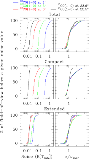
Figure 11.— Cumulative histograms of the rms noise for the ¹³CO (1–0) (dashed line) and ¹²CO (1–0) (solid lines) cubes. The IRAM-30m cubes are displayed in black, the interferometric cubes at 1, 3, and $6^{\prime\prime}$ are displayed in blue, green, and red, respectively. Top: Hybrid synthesis or IRAM-30m data cubes. Middle: PdBI-only data cubes or the $6^{\prime\prime}$ extended data cube smoothed to $22.5^{\prime\prime}$ and subtracted from the IRAM-30m cube. Bottom: PdBI-only cubes subtracted from the hybrid synthesis cubes or the $6^{\prime\prime}$ PdBI-only data cube smoothed to $22.5^{\prime\prime}$ and subtracted from the IRAM-30m cube. Left: Histograms of absolute noise values. Right: Histograms of noise normalized by the median noise value.

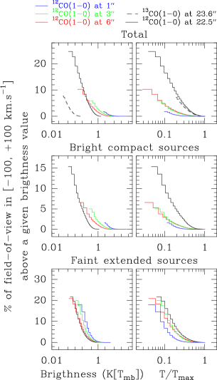
Figure 12.— Cumulative histograms of the signal above the $5\sigma$-level for the ¹³CO (1–0) (dashed line) and ¹²CO (1–0) (solid lines) cubes. The IRAM-30m cubes are displayed in black, the interferometric cubes at 1, 3, and $6^{\prime\prime}$ are displayed in blue, green, and red, respectively. Top: Hybrid synthesis or IRAM-30m data cubes. Middle: PdBI-only data cubes or the $6^{\prime\prime}$ extended data cube smoothed to $22.5^{\prime\prime}$ and subtracted from the IRAM-30m cube. Bottom: PdBI-only cubes subtracted from the hybrid synthesis cubes or the $6^{\prime\prime}$ PdBI-only data cube smoothed to $22.5^{\prime\prime}$ and subtracted from the IRAM-30m cube. Left: Histograms of raw brightnesses. Right: Histograms of brightnesses normalized to the maximum brightness.

In order to quantify the $(l,m,v)$-volume filling factors and the beam dilution properties of the compact and extended emission, we now describe the distribution of the noise and brightness values.

Figure 11 displays the cumulative histograms of the rms noise for the 4 different resolutions (1, 3, 6, and $22.5^{\prime\prime}$), and for the 3 kind of cubes: Hybrid synthesis (top), PdBI-only (middle) and subtracted (bottom). The left column displays the raw histograms while the right column presents the histograms normalized by their median value, as this eases the comparison of shapes. The histograms show that the noise distributions are well centered on the median value, implying relatively uniform noise properties. The IRAM-30m single-dish data display an increase of the histogram population at high noise values because the noise distributions are homogeneous over the inner $400^{\prime\prime}\times 400^{\prime\prime}$ field of view but they increase on the northern and southern patch. A similar effect is seen for the interferometric data, which is directly linked to a noise increase at the edges of the field because of the correction of primary beam attenuation. Moreover, in the single-dish data, the ¹²CO median noise level (16$\,\mathrm{mK}$) is about twice as high as the ¹³CO one (7.5$\,\mathrm{mK}$) because the ¹²CO (1–0) line is closer to an oxygen atmospheric line.

The brightness noise levels of the hybrid synthesis data cubes are mostly set by the interferometric radiometric noise because the increase of integration time from the IRAM-30m to the PdBI does not match the gain in angular resolution (see Sect. 2.3.2). Hence, the median rms noise (see Table 4) and the noise cumulative histograms (see Fig. 11) are almost identical for the PdBI-only and hybrid synthesis data cubes. On the other hand, the brightness noise levels for the subtracted data cubes are mostly set by the single-dish data. Indeed, we subtracted two data sets whose noise is partially correlated: The noise coming from the PdBI visibilities is common. Subtracting both data cubes result in noise properties close to the IRAM-30m noise properties. In particular, the median rms noise in the subtracted data cube is more than one order of magnitude smaller than the median rms noise of the hybrid synthesis cube at $1^{\prime\prime}$ resolution.

Figure 12 shows the cumulative histograms of the cube brightness using a similar layout as Fig. 11. In the right column, the histograms are normalized by the maximum brightness. The histograms were computed using the full PAWS field of view but only the parts above the $5\sigma$ brightness noise level are displayed. The hybrid synthesis and PdBI-only histograms are similar both qualitatively and quantitatively. The histograms are displaced towards higher brightness values when the angular resolution increases, implying that all the structures above the $5\sigma$ noise levels experience large beam dilution effects. For example, the maximum brightness increases by more than one order of magnitude from 1.3 to 16$\,\mathrm{K}$, when increasing the resolution from 22.5 to $1^{\prime\prime}$. On the other hand, the histograms of the subtracted cubes are identical within the noise constraints (even for the normalized histogram of the $1^{\prime\prime}$ cube as the value of the maximum brightness is relatively uncertain). Indeed, the maximum brightness of the extended component evolves only from $0.97\pm 0.07$ to $1.36\pm 0.07\,\mathrm{K}$ from $22.5^{\prime\prime}$ (the IRAM-30m resolution) to $6^{\prime\prime}$ (the PAWS resolution for which the extended emission is best defined). This implies that beam dilution is negligible for the subtracted emission. This is consistent with this emission being structured mostly at spatial scales larger than $36^{\prime\prime}$.

The $(l,m,v)$-volume filling factors and the median brightness values were computed on all the cube pixels with detected signal, i.e. their brightness is larger than 5 times their noise. Using this definition, the brightness of the compact component (measured on the $1^{\prime\prime}$ PdBI-only cube) ranges from 2.0 to 16.0$\,\mathrm{K}$, with a median value of 2.5$\,\mathrm{K}$ and it fills less than 2% of the $(l,m,v)$-volume. The brightness of the extended component (measured on the $6^{\prime\prime}$ subtracted cube) ranges from 0.07 to 1.36$\,\mathrm{K}$, with a median value of 0.14$\,\mathrm{K}$ and it fills $\sim 30\%$ of the $(l,m,v)$-volume.

The comparison of the noise and signal distributions of the cubes at different angular resolutions makes it clear why the deconvolution of the PdBI-only data recovers more flux at $3^{\prime\prime}$ than $1^{\prime\prime}$ but almost the same flux at $6^{\prime\prime}$ and $3^{\prime\prime}$. Indeed, the subtracted emission has a median brightness of 0.14$\,\mathrm{K}$, which is $\sim 0.35$ times the hybrid synthesis brightness noise level at $1^{\prime\prime}$ but $\sim 1.3$ and 4 times the hybrid synthesis noise level at $3^{\prime\prime}$ and $6^{\prime\prime}$, respectively. In other words, any emission present in the PdBI-only data is only recovered when its signal-to-noise is large enough (typically $\geq 5$).

3.2.2 Spatial distribution of the line moments

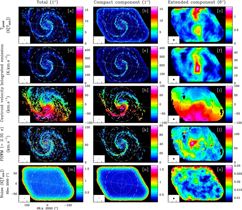
Figure 13.— Comparison of the spatial distribution (from top to bottom) of the peak intensity, integrated intensity, centroid velocity, the line full width at half maximum (i.e., 2.35 times the standard deviation in velocity), and rms noise of the ¹²CO (1–0) emission for the hybrid synthesis (PdBI + 30m, left column) and the PdBI-only (middle column) cubes at $\sim 1^{\prime\prime}$ resolution, and the $6^{\prime\prime}$-resolution subtracted cube (right column). The angular resolution is indicated by a circle in the bottom left corner of each panel. The intensity scale is shown on the right-hand side of each panel. The major and minor axes are displayed as perpendicular dotted lines. The dotted circles show the two inner corotation resonances at radii equal to $23^{\prime\prime}$ and $55^{\prime\prime}$, while the dashed circle indicates the start of the material arms at a radius equal to $85^{\prime\prime}$ (Meidt et al., 2013).

Figure 13 summarizes the properties of the decomposition of the total emission into the compact and the extended emission. The spatial distributions of the peak temperature, line integrated emission (the 0th order moment), centroid velocity (the 1st order moment), line full width at half maximum (computed as 2.35 times the line 2nd order moment), and the noise are presented from top to bottom. The total and compact emissions are presented at the best possible PAWS resolution ($1^{\prime\prime}$), while the extended emission is displayed at the resolution where it is best measured, i.e., $6^{\prime\prime}$. Figures 32, 33, 34, and 35 (available in the electronic version only) show the same decomposition at fixed angular resolutions from 1, 3, 6, and $22.5^{\prime\prime}$, respectively. This demonstrates how the different moments of each component of the emission vary with spatial resolution.

The deconvolved intensity distribution is corrected for primary beam attenuation, which makes the noise level spatially inhomogeneous. In particular, the noise strongly increases near the edges of the field of view (see, e.g., panels [m] to [o] of Fig. 13). To limit this effect, the deconvolved mosaic is truncated at its edge, giving an almost parallelogram field of view of $\sim 10.5$ square arcminutes. A comparison with the IRAM-30m data (Fig. 35[a-f]) shows that signal is present near or slightly beyond the edges of the PAWS field of view. This implies that the signal at the edge of the PAWS field of view is probably less well deconvolved from the contribution of emission outside the PAWS field of view. This effect is more important at the northern edge and to a lesser extent at the southern edge than at the western and eastern edges.

Two kinds of artifact appear in the peak temperature and integrated intensity maps of the $1^{\prime\prime}$ subtracted cube, which shows the extended component. First, a moire effect due to the undersampling of the field pointings in the mosaic appears as a slight modulation of the intensity at a typical spatial scale of $\sim 18^{\prime\prime}$ (see Fig. 32[f]). This is due to power aliasing in the $uv$ plane (Pety & Rodríguez-Fernández, 2010). Second, the chicken-pox aspect at a spatial scale close to the synthesized resolution is a known artifact of the deconvolution method that we used (see Fig. 32[c]). The overall spatial repartition of the extended component is nevertheless correct as evidenced by the comparison with the spatial distributions of the moments at $3^{\prime\prime}$ and $6^{\prime\prime}$, where the impact of these artifacts becomes negligible.

The subtracted cube reveals extended emission whose peak temperature distribution is barely detected in the $1^{\prime\prime}$ hybrid synthesis cube, as the signal-to-noise ratio of this emission ranges between 0.2 and 3.5 (see Fig. 13[a-c]). This is why a relatively complex dedicated masking technique was devised to compute meaningful 1st and 2nd order moments for the $1^{\prime\prime}$ hybrid synthesis cube (see Section B for a detailed description). The peak temperature (Fig. 13[c]) and integrated emission (Fig. 13[f]) maps are maximum along the major axis of the galaxy. This is expected because emission in a given velocity channel extends over a large 2D area near the major axis, while is mostly extended in one spatial dimension along the minor axis. Hence, the interferometer will recover “extended” emission along the minor axis much better than along the major axis. This projection effect thus minimizes emission along the minor axis in the subtracted cube. However, there is more than a major axis trend in the subtracted cube. Indeed, Figure 30 and 31 (available in the electronic version only) show an overlay of the signal-to-noise contours of the $1^{\prime\prime}$ PdBI-only data cube onto the signal of the $6^{\prime\prime}$ subtracted cube for a set of channels at negative and positive velocities. These figures suggest that the extended emission fills the central $55^{\prime\prime}$, bounded by the inner edge of the spiral arms, and then falls on the convex side of the arms at larger radii (out to $\sim 85^{\prime\prime}$).

While the peak temperature map exhibits a symmetric spatial distribution relative to the galaxy center, the integrated emission peaks in the southern part. Extended emission is completely absent in the $1^{\prime}\times 1^{\prime}$-areas located roughly southwest $(-60^{\prime\prime},-20^{\prime\prime})$ and northeast $(+60^{\prime\prime},+40^{\prime\prime})$ of the center. The maps of centroid velocity indicate differences between the kinematics of the compact and extended emission. This is best seen when following the 0$\,\mathrm{km\,s^{-1}}$-isovelocity line, i.e., NGC 5194’s systemic velocity, on Fig. 34[h and i] or on Fig. 35[h and i]. The linewidth of the extended component (Fig. 13[l]) is largest inside a central circle of $\sim 35^{\prime\prime}$ radius. Linewidths are on average much larger for the extended than for the compact emission. The clearest exception is at the galaxy center, i.e., at radii smaller than $2.5^{\prime\prime}$, where the compact emission has high peak temperature, large linewidth, and large integrated emission. This is reminiscent of the properties of molecular gas in the inner 180$\,\mathrm{pc}$ of our Galaxy (Morris & Serabyn, 1996). Alternatively, Kohno et al. (1996) and Matsushita et al. (2004) interpret these as gas being entrained by the AGN radio jet.

We verified that the large linewidth of the extended component is not caused by the contribution from the error beams. Details are provided in the Appendix C.3.

3.2.3 Azimuthal averages

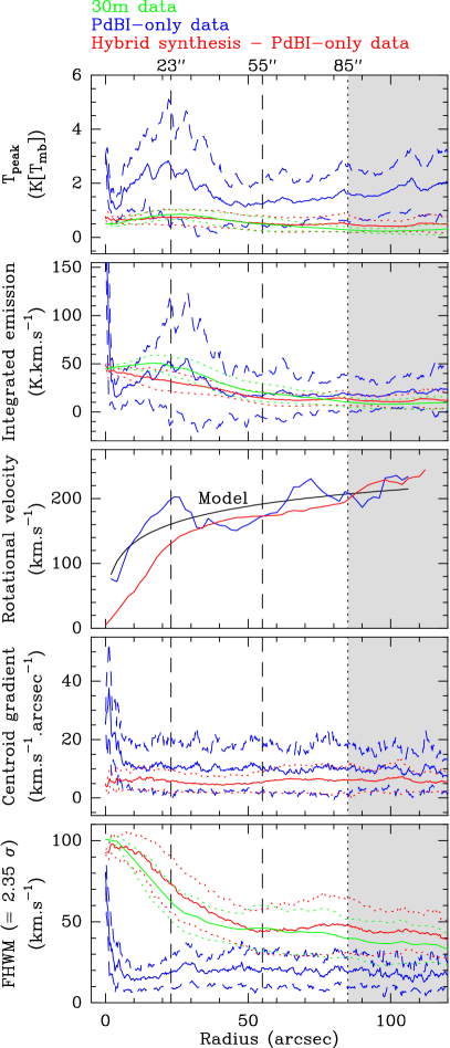
Figure 14.— Deprojected azimuthal averages around the kinematic center for the IRAM-30m (green curves), the PdBI-only (blue curves) and the subtraction of the PdBI-only from the hybrid synthesis (red curves) cubes. The solid lines display the averages while the dashed lines give the azimuthal averages plus/minus the azimuthal standard deviations. From top to bottom, the panels present the peak temperature, line integrated emission, the rotational velocity, the modulus of the centroid velocity gradient, and 2.35 times the line 2nd order moment as a function of radius. The vertical dashed lines indicate the two inner corotation resonances at radii equal to $23^{\prime\prime}$ and $55^{\prime\prime}$, while the vertical dotted line show the start of the material arms at a radius equal to $85^{\prime\prime}$ (Meidt et al., 2013). The radial zone where the averages are affected by edge effects (see Sect. 3.2.3) is highlighted in grey.

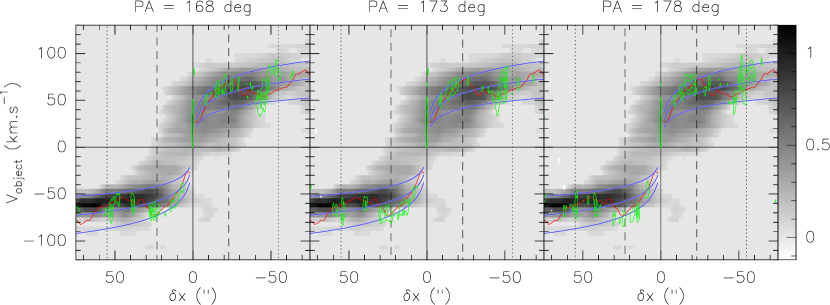
Figure 15.— Position-velocity diagrams of the extended emission (hybrid synthesis minus PdBI-only) imaged at $6^{\prime\prime}$ along 3 axes at PA $=173\arcdeg$ (major axis, central panel), and $173\pm 6\arcdeg$ (left and right panels) shown in grey-scale. The scale is shown in the right-hand side ($\,\mathrm{K}$ [$T_{\mathrm{mb}}$]). The green contours (at levels 2, 4, 6, 8, 10 $\,\mathrm{K}$ [$T_{\mathrm{mb}}$]) display the hybrid synthesis emission at $1^{\prime\prime}$ resolution. The red curve is the azimuthally averaged rotational velocity profile and the central blue curve is a smooth 3-parameters fit of the red curve with a fixed inclination of $21\arcdeg$. The two other blue curves diplay the same model but for an inclination of $15\arcdeg$ and $27\arcdeg$. The vertical lines show the two inner corotation resonances at a radius of $23^{\prime\prime}$ and $55^{\prime\prime}$ (Meidt et al., 2013).

Figure 14 shows the azimuthal average (and the associated dispersion) around the kinematic center of the deprojected images of the peak temperature, the integrated emission, the rotational velocity, the modulus of the centroid velocity gradient, and the line full width at half maximum computed for the $1^{\prime\prime}$ PdBI-only (blue curves), the $1^{\prime\prime}$ subtracted (red curves), and the $22.5^{\prime\prime}$ IRAM-30m (green curves) cubes.

For the compact emission (PdBI-only cube), the inner $5^{\prime\prime}$ clearly display high peak temperatures and large FWHMs, implying large integrated line emissions. The molecular ring dominates from $\sim 10$ to $40^{\prime\prime}$, where the integrated emission and the peak temperatures are larger than in the disk (radii larger than $\sim 40^{\prime\prime}$). The peak temperature seems to increase from the ring to the outer disk, while the integrated emission stays mostly constant outside $r\sim 80^{\prime\prime}$. On the other hand, the velocity FWHM decreases slightly from $\sim 25\,\mathrm{km\,s^{-1}}$ at a radius of $\sim 30^{\prime\prime}$ to $20\,\mathrm{km\,s^{-1}}$ at radii larger than $\sim 100^{\prime\prime}$.

The extended emission (subtracted cube) has a typical peak temperature of 0.75$\,\mathrm{K}$ in the central region and 0.5$\,\mathrm{K}$ in the disk. The FWHM decreases by a factor of 2 from $\sim 100\,\mathrm{km\,s^{-1}}$ at $0^{\prime\prime}$ to $\sim 45\,\mathrm{km\,s^{-1}}$ at $50^{\prime\prime}$ and it then varies between 40 and 50$\,\mathrm{km\,s^{-1}}$ in the outer disk. Both properties result in a regular decrease of the integrated emission from $\sim 45\,\mathrm{K\,km\,s^{-1}}$ at the center to $\sim 15\,\mathrm{K\,km\,s^{-1}}$ at $50^{\prime\prime}$. It then varies between 10 and 15$\,\mathrm{K\,km\,s^{-1}}$.

The compact emission has on average a peak temperature twice as large as the extended emission. In contrast, the extended emission has a velocity FWHM at least twice as large as the compact emission (except near the center). Both effects almost compensate to yield similar integrated line emissions for both components.

The dispersion of the peak temperature and of the integrated emission is larger for the compact emission than for the extended one. This is a consequence of the fact that the compact emission is structured at all scales down to or below the angular resolution while the filtered flux is structured mostly at scales larger than $36^{\prime\prime}$. The dispersion of the FWHM measurement is similar in both the compact and extended emissions. Indeed, its azimuthal average is computed only where there is enough signal to define it (i.e., on a small fraction of $360\arcdeg$), while the peak temperature and integrated emission are averaged over $360\arcdeg$ (at least up to a radius of $85^{\prime\prime}$).

The rotation velocity of each component was measured by fitting tilted rings with fixed systemic velocity to the line-of-sight velocity field using the GIPSY task ROTCUR. In both cases, we assume the kinematic center listed in Table 1, and we adopt a constant position angle $(173^{\circ}{})$ and inclination $(21^{\circ})$, as estimated from the more radially extended Hi emission mapped at lower resolution by the THINGS project (see Colombo et al., 2013b, for more details). The middle black curve, labeled “Model”, is a 3-parameter fit of the measured rotation curve. The inner part of this fit (inside $100^{\prime\prime}$) compares well with what we would expect if the stars (traced at 3.6$\,\mathrm{\mu{}m}$) dominate the baryonic mass (Meidt et al., 2013).

The rotational velocity of the extended emission (red curve) is increasing almost monotonically with radius, while it oscillates twice for the compact emission (blue curve) as an effect of the streaming motions and corotation resonances (and not the bulge). Moreover, the centroid velocity of the extended emission is typically closer to NGC 5194’s systemic velocity by 50$\,\mathrm{km\,s^{-1}}$ at radii smaller than $35^{\prime\prime}$ where an inner stellar bar dominates the dynamics. At larger radii, it overlaps the rotational velocity curve of the compact emission. The modulus of the centroid velocity gradient is around 6 and $10\,\mathrm{km\,s^{-1}}/^{\prime\prime}$ for the extended and compact components, respectively. Hence, the kinematics of the extended emission vary much more smoothly on the plane of the sky than the kinematics of the compact emission, which is very much affected by streaming motions (This is further discussed in Sect. 3.3.3).

Any intrinsic behavior beyond a radius of $85^{\prime\prime}$ must be interpreted with caution as the azimuthal averages reach the edges of the field of view in its smallest dimension. Two effects happen: 1) The noise increases sharply at the mosaic edges (see the bottom left panel of Fig. 13), and 2) the azimuthal averages miss the outside interarm regions, which occupy a larger and larger fraction of the area as the distance from the center increases. However, the comparison of the averages of the extended and compact emission at each radius is meaningful as the averages are made on the same ellipse portions.

3.2.4 Kinematics along the major axis

Figure 15 compares the position-velocity diagrams along the major axis of the compact emission (PdBI-only, green contours) and the extended (grey image) emission. The red curve is the measured rotation curve. It matches well the overall velocity variation along the major axis. The middle blue curve is the 3-parameter fit of the measured rotation curve, implying an overall inclination of the galaxy on the plane of sky of $21\pm 3\arcdeg$ (see Sect. 3.2.3). The two other blue curves show the same velocity model for inclinations of $15\arcdeg$ and $27\arcdeg$, in order to give an indication of the effect of inclination on the kinematics.

This diagram confirms that the linewidth is much larger for the extended than for the compact emission (with the possible exception of the molecular gas at the center of the galaxy). The extended emission has a parallelogram shape with gas emitting at forbidden velocity in the $[-35^{\prime\prime},+35^{\prime\prime}]$ radius range. This is a typical signature of nuclear bar kinematics (e.g., Binney et al., 1991; Garcia-Burillo & Guelin, 1995; Garcia-Burillo et al., 1999). The distribution of the extended emission in PV-space might in addition or otherwise indicate that it lags the compact emission. The parallelogram shape is not symmetric, and emission is absent in the region near $(+15^{\prime\prime},-25\,\mathrm{km\,s^{-1}})$. At and inside this position (and its mirror, near $-15^{\prime\prime}$), emission in the extended component that falls below the rotational velocities exhibited by the compact emission (red curve) might arise with a genuine lag.

3.3. Interpretation 1: Two CO disks – Thin and thick

After an intermediate summary of the main observational properties of the two CO emission components, we will translate them into physical properties of the gas traced by the ¹²CO (1–0) emission. To do this, we will first summarize the expressions for the gas scale height, mid-plane pressure and gas density as a function of the gas and stellar surface densities and vertical velocity dispersions (Koyama & Ostriker, 2009). We will then discuss how to apply these expressions to M51. In particular, we will show how the contribution of the streaming motions to the CO linewidth can be estimated to derive an accurate vertical gas velocity dispersion.

3.3.1 Intermediate summary and consistency checks

The emission filtered out by the PdBI interferometer accounts for about half of the total flux imaged in the hybrid (PdBI+30m) synthesis. The subtraction of the PdBI-only from the hybrid synthesis cubes shows ¹²CO (1–0) emission mostly structured at angular scales larger than $36^{\prime\prime}$, i.e., $\sim 1.3\,\mathrm{kpc}$. Its brightness temperature ranges from 0.1 to 1.4$\,\mathrm{K}$ with a median value of 0.14$\,\mathrm{K}$. It covers about 30% of the PAWS field of view. Its spatial distribution surrounds the bright spiral arms. While the integrated line emission peaks at 48$\,\mathrm{K\,km\,s^{-1}}$ near the major axis in the south-western galaxy quadrant, the peak brightness along the major axis ranges from 0.7 to 1.4$\,\mathrm{K}$ in the northeast and 0.5 to 0.8$\,\mathrm{K}$ in the south-western quadrant. This emission is thus faint and extended. In contrast, the emission observed by the interferometer is compact and bright. Indeed, its brightness temperature ranges from 2 to 16$\,\mathrm{K}$ with a median value of 2.5$\,\mathrm{K}$ and it covers less than 2% of the PAWS field of view. Rotational velocities estimated from the centroid velocity map of the extended component are closer by $50-100\,\mathrm{km\,s^{-1}}$ to the systemic velocity than the ones of the compact component inside a circle of $35^{\prime\prime}$ radius. Outside this radius, the rotational velocities of both components have the same order of magnitude. But, the rotational velocity curve of the compact component oscillates around the modeled velocities, while the rotational velocity curve of the extended component smoothly increases and mostly lies below the modeled velocities. The line FWHM of the extended component is twice as large as that of the compact component.

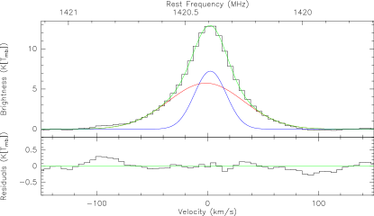
Figure 16.— Dual Gaussian decomposition of the THINGS HI spectrum averaged over the PAWS field of view after having aligned all the individual spectra along the velocity axis according to their centroid velocity value. Top: Brightness of the average spectra as a black histogram. The dual Gaussian fit is displayed as the green line and the two individual Gaussians are shown in red and blue. Bottom: Residual brightness after subtraction of the dual Gaussian fit.

Table 6Results of the dual Gaussian fit (see Fig. 16).

Gaussian	$T_{\mathrm{peak}}$	Velocity	Width	Area
#	(K[$T_{\mathrm{mb}}$])	($\,\mathrm{km\,s^{-1}}$)	($\,\mathrm{km\,s^{-1}}$)	($\,\mathrm{K\,km\,s^{-1}}$)
1	5.7	$-1.4\pm 0.4$	$80\pm 2$	$490\pm 13$
2	7.2	$+2.5\pm 0.2$	$34\pm 1$	$260\pm 14$

We made two additional consistency checks. First, CPROPS decomposes the $1^{\prime\prime}$ hybrid synthesis cube into two different components: 1) “Clouds” which account for 55% of the total flux, and 2) “Intercloud” gas which “surrounds” the GMCs and accounts for the remaining flux (Colombo et al., 2013a). These numbers remain stable when the analysis is done using the $6^{\prime\prime}$ hybrid synthesis cube. This decomposition result reflects the fact that we have a faint extended component in addition to the bright compact ¹²CO emission. Second, we checked whether existing Hi observations are consistent with the possibility of having a narrow and broad linewidth component. We started from the THINGS Hi cube imaged at $11.9^{\prime\prime}\times 10.0^{\prime\prime}$ resolution with natural weighting (Walter et al., 2008), as it maximizes the signal-to-noise ratio. We applied the shuffle method of Schruba et al. (2011), i.e., we shifted each spectrum of the Hi cube to a common velocity scale by removing the systematic velocity field structure as measured from the centroid velocity. The spectra were then averaged over the PAWS field of view. Only a dual Gaussian can accurately fit the Hi spectrum. Figure 16 displays the shuffled, averaged spectrum, its Gaussian decomposition and the residuals. Table 6 presents the quantitative results of the dual Gaussian fit. The total flux is divided approximately equally in both components while the FWHM is approximately twice as large in one of the components. This is consistent with a separation into two emission components with very different linewidths.

3.3.2 Expressions for the gas scale heights, mid-plane pressures, and gas densities

Using the vertical momentum and Poisson equations averaged over the horizontal plane of the galaxy, Koyama & Ostriker (2009) obtained a second-order differential equation for the averaged vertical density profile. Solving it, they showed the averaged gas density ($\rho$) and pressure ($P$) are approximately given by Gaussian profiles of the height $z$, i.e.,

$$\rho(z)=\rho_{0}\,\exp\displaystyle\left(-\frac{z^{2}}{2H_{\mathrm{}}^{2}}\right)\quad\mbox{and}\quad P(z)=P_{0}\,\exp\displaystyle\left(-\frac{z^{2}}{2H_{\mathrm{}}^{2}}\right).$$ (1)

In these equations, the gas scale height $H_{\mathrm{}}$ is given by

$$H_{\mathrm{}}=\frac{\sigma_{z}}{\sqrt{4\pi G\,\rho_{\star}}}\frac{1}{A+\sqrt{A^{2}+1}},$$ (2)

where $\sigma_{z}$ is the thermal plus turbulent velocity dispersion perpendicular to the galactic disk, $\rho_{\star}$ is the stellar density, $G$ is the gravitational constant, and $A$ is a dimensionless factor that measures the relative densities of the gaseous and stellar disks. It can be expressed as

$$A=\sqrt{\frac{G\,\Sigma_{\mathrm{gas}}^{2}}{2\rho_{\star}\,\sigma_{z}^{2}}},$$ (3)

where $\Sigma_{\mathrm{gas}}$ is the gas surface density. Once the gas vertical scale height is known, the gas mid-plane density and pressure can easily be derived with

$$\rho_{0}=\frac{\Sigma_{\mathrm{gas}}}{\sqrt{2\pi}\,H_{\mathrm{}}}\quad\mbox{and}\quad P_{0}=\sigma_{z}^{2}\,\rho_{0}.$$ (4)

These expressions for the gas scale height, mid-plane pressure, and mid-plane density take into account 1) gravity forces that both the stars and gas exert, and 2) turbulent and thermal hydrodynamic pressures. However, they still are lower limits as they neglect any contribution from the magnetic field.

Finally, for an isothermal, self-gravitating stellar disk, the stellar surface density, the stellar volume density, the stellar vertical scale height, $H_{\mathrm{\star}}$, and the stellar vertical velocity dispersion, $\sigma_{\star}$, are linked via

$$\rho_{\star}=\frac{\Sigma_{\star}}{2H_{\mathrm{\star}}},\quad\mbox{and}\quad H_{\mathrm{\star}}=\frac{\sigma_{\star}^{2}}{\pi G\,\Sigma_{\star}}.$$ (5)

The A factor can then be rewritten as

$$A\sim\frac{Q_{\star}}{Q_{\mathrm{gas}}},$$ (6)

where $Q_{\star}$ and $Q_{\mathrm{gas}}$ are the Toomre’s gravitational stability parameters for the stellar and gas disks.

3.3.3 Application to M51

Figure 17 displays how the previous expressions are applied to the case of M51 as a function of galactocentric radius for the total gas at $22.5^{\prime\prime}$ resolution (green curves), the extended component at $6^{\prime\prime}$ resolution (red curves) and the compact component at $1^{\prime\prime}$ resolution (blue curves). Radial zones where the results should be interpreted with caution are highlighted in grey: 1) at radii larger than $85^{\prime\prime}$, the azimuthal averages start to reach the edges of the observed field of view; and 2) from 0 to $\sim 45^{\prime\prime}$, the assumption that the stars are distributed in a disk breaks down, so that the stellar scale height and volume density are not well constrained (see below).

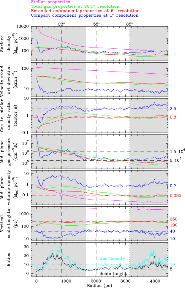
Figure 17.— Azimuthal averages around the kinematic center, from top to bottom: Mass surface densities, vertical velocity standard deviations (i.e., line full width at half maximum divided by 2.35), gas-to-stellar density ratios (A factor), gas thermal + turbulent mid-plane pressures, gas mid-plane densities, vertical scale heights for the stars (pink curves), the IRAM-30m (green curves), the PdBI-only (blue curves) and the subtracted (red curves) cubes. The bottom panel displays the ratios of the scale heights (black) and mid-plane densities (cyan) computed from the PdBI-only and subtracted data sets. The horizontal lines indicates typical values of the different parameters for the compact and extended components. The vertical dashed lines indicate the two inner corotation resonances at radii equal to $23^{\prime\prime}$ and $55^{\prime\prime}$, while the vertical dotted line show the start of the material arms at a radius equal to $85^{\prime\prime}$ (Meidt et al., 2013). The radial zones where the results should be interpreted with caution (see Sect. 3.3.3) are highlighted in grey.

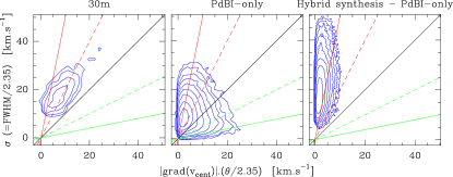
Figure 18.— Joint distributions of the line 2nd order moment as a function of the centroid velocity gradient modulus times the half primary beam width for the 30m (left), PdBI-only (middle) and subtracted (right) cubes. The lines have a slope of 0.2 (green, solid), 0.5 (green, dashed), 1 (black, solid), 2 (red, dashed), and 5 (red, solid).

The gas mass surface densities for each component are computed from the azimuthal averages of the ¹²CO (1–0) integrated emission using the Galactic value of the $X_{\mathrm{CO}}$ factor and taking into account the presence of helium. The stellar surface density is derived from the 3.6$\,\mathrm{\mu{}m}$ emission (Meidt et al., 2012). The stellar velocity is computed following Bottema (1993) and Boissier et al. (2003) who showed that, for a flat exponential disk, it falls off from the central dispersion $\sigma_{0}$ according to

$$\sigma_{\star}=\sigma_{0}\,\exp\displaystyle\left(-\frac{r}{2\,H_{B}}\right),$$ (7)

where $r$ is the galaxy radius and $H_{B}$ is the disk scale length of the $B$-band. McElroy (1995) estimates the central stellar velocity dispersion in M51 to be $\sigma_{0}=113\,\mathrm{km\,s^{-1}}$ and Trewhella et al. (2000) estimates that $H_{B}=2.82\,\mathrm{kpc}$. This gives us an estimate for the stellar scale height and volume density, according to Eq. 5. We emphasize that this assumes an isothermal, self-gravitating stellar disk. This assumption clearly breaks down in the center of M51, where the bulge and nuclear bar dominate, i.e., at radii less than $\sim 25^{\prime\prime}$ where the 3.6$\,\mathrm{\mu{}m}$ surface brightness profile exhibits steepening, and near the location of the bar corotation radius as estimated from gravitational torques (Meidt et al., 2013). In fact, the application of Eq. 5 results in a stellar scale height that decreases with radius from $\sim 45^{\prime\prime}$ to the galaxy center. We therefore opted to adopt a constant, lower limit to the scale height inside this zone by extrapolating the value given by Eq. 5 at a radius of $45^{\prime\prime}$ inward.

The vertical velocity dispersion of the gas can be estimated as the line 2nd order moment for a face-on galaxy. The inclination of M51 onto the line of sight is small but non-zero, implying that the line 2nd order moment is only a first order approximation. Indeed, the systematic motions averaged inside the beam of the observations contribute to the line 2nd order moment. This is more problematic in the case of M51 because the streaming motions are known to be large for this galaxy. Appendix D shows that the vertical velocity dispersion can be estimated as

$$\sigma_{z}^{2}\sim\displaystyle\left<\displaystyle\left(v_{\mathrm{obs}}-v_{\mathrm{cent}}\right)^{2}\right>-\displaystyle\left[\displaystyle\left|\mathbf{\mathrm{grad}(v_{\mathrm{cent}}{})}\right|{}\,\frac{\theta}{2.35}\right]^{2},$$ (8)

where $\displaystyle\left<\right>$ symbolizes the brightness-weighted average over the line profile, $v_{\mathrm{obs}}$ is the velocity projected along the line of sight, $v_{\mathrm{cent}}$ the line centroid velocity, $\displaystyle\left|\mathbf{\mathrm{grad}(v_{\mathrm{cent}}{})}\right|$ the modulus of the gradient of the centroid velocity, and $\theta$ the resolution beamwidth of the observations. In this equation, the first term is the square of the second moment and the second term estimates the contribution of unresolved systematic motions.

Figure 18 diplays the joint distributions of these two quantities for the IRAM-30m cube and the $1^{\prime\prime}$ PdBI-only and subtracted cubes. At the resolution of the IRAM-30m data, the unresolved systematic motions contribute significantly to the value of the second moment. This behavior is clearly split in the decomposition between compact and extended components at $1^{\prime\prime}$. The unresolved systematic motions are negligible for the extended component. For the compact component, they contribute to less than 34% of the linewidth for 50% of the data. Hence, the streaming motions are seen in the compact component but they are not seen in the extended component. We stress that the subtracted cube measures the extended component at an angular resolution of $1^{\prime\prime}$ because it results from the subtraction of two cubes whose resolution is $1^{\prime\prime}$, namely the hybrid synthesis and the PdBI-only cubes. Beam smearing of unresolved systematic motions must therefore be considered only at angular scales lower than $1^{\prime\prime}$. As a corollary, if the large linewidths are due to beam smearing of unresolved streaming motions, then the linewidths should decrease when increasing the imaging angular resolution. This effect is observed in both the hybrid synthesis and PdBI-only cubes (panels [j] and [k] of Fig. 32 to 34), while the second moment of the subtracted cube (panels [l] of the same figures) stays basically constant when increasing the angular resolution from $22.5^{\prime\prime}$ to $1^{\prime\prime}$. We thus deduced that the large linewidths of the extended component are not caused by unresolved streaming motions.

As the unresolved systematic motion can be larger than the second moment for the compact component, we only used the second moments to compute the vertical velocity dispersion, implying that the scale heights and mid-plane pressures derived are slightly more robust for the extended component than for the compact component and the IRAM-30m data.

3.3.4 Results

Using these inputs, we computed the stellar vertical scale height, and volume density. We also computed the gas-to-stellar density ratio ($A$ factor), the gas mid-plane pressures, densities, and scale heights for all the molecular gas (using the IRAM-30m data), the compact component (using the PdBI-only data), and the extended component (using the subtracted cube). We neglect the contribution from atomic gas traced by Hi emission, as this gas represents only between 2.5 and 30% of the molecular gas mass for radii from 0 to $130^{\prime\prime}$ (see Fig. 42 of Leroy et al., 2008; Schuster et al., 2007).

Our estimates agree very well with expectations. For example, the A factor is less than 1 for the extended component, while it is equal to $\sim 2.5$ for the compact component for radii larger than 0.5$\,\mathrm{kpc}$. Using Eq. 6, this implies that $Q_{\mathrm{compact}}\sim 0.3Q_{\mathrm{extended}}$, where $Q_{\mathrm{compact}}$ and $Q_{\mathrm{extended}}$ are the Toomre factors for the compact and extended components, respectively. Said otherwise, the compact component is more likely to form stars than the extended component. The gas mid-plane pressure is about the same for both components and for the total gas. This probably reflects pressure equilibrium. From the mid-plane pressure, we estimate a molecular fraction $\Sigma_{\mbox{H${}_{2}$}}/\Sigma_{\mbox{H{\sc i}}}$ close to what is observed: Using the empirical formula which relates the molecular fraction $\Sigma_{\mbox{H${}_{2}$}}/\Sigma_{\mbox{H{\sc i}}}$ to the mid-plane pressure (Blitz & Rosolowsky, 2006)

$$\Sigma_{\mbox{H${}_{2}$}}/\Sigma_{\mbox{H{\sc i}}}=\displaystyle\left(\frac{P_{0}}{4.3\times 10^{4}\,\mathrm{K\,cm^{-3}}}\right)^{0.92},$$ (9)

we find a molecular fraction of $\sim 26$ and $\sim 4$ at radii equal to 1.0 and 2.5$\,\mathrm{kpc}$, respectively, in good agreement with the results of Leroy et al. (2008). Based on the high molecular fraction, we thus expect a tight correlation between the star formation rate and the molecular gas surface density, but probably little relation to the atomic gas surface density, as found by Kennicutt et al. (2007).

The scale height of the extended component is almost constant, its value varying slighty betwen 190 and 250$\,\mathrm{pc}$ for radii larger than 0.5$\,\mathrm{kpc}$. The scale height of the compact component varies more. It is $\sim 40\,\mathrm{pc}$ between $\sim 1.5$ and 3.5$\,\mathrm{kpc}$. It varies between $\sim 20$ and 40$\,\mathrm{pc}$ beyond $\sim 3.5\,\mathrm{kpc}$ and it decreases to $\sim 10\,\mathrm{pc}$ at $\sim 0.5\,\mathrm{kpc}$. In other words, the scale height of the compact emission is 5-6 times smaller than the scale height of the extended component from $\sim 1.5$ to $3.5\,\mathrm{kpc}$. The compact component is between 5 and 20 times (typically 10 times) denser than the extended component. At a radius of 2.5$\,\mathrm{kpc}$, the extended and compact components have an average volume density of $\sim 1$ and 10 H₂ $\,\mathrm{cm^{-3}}$, respectively. For reference, the distribution of the molecular gas density in the Solar Neighborhood is (Ferrière, 2001; Cox, 2005)

$$\frac{n}{\mbox{H${}_{2}$}\,\,\mathrm{cm^{-3}}}=0.29\,\exp\displaystyle\left[-(z/81\mathrm{pc})^{2}\right],$$ (10)

i.e., a scale height of $57\,\mathrm{pc}(=81\,\mathrm{pc}/\sqrt{2})$ and a mid-plane gas density of 0.29 H₂ $\,\mathrm{cm^{-3}}$. The volume density is several orders of magnitude smaller than the expected densities of molecular gas. This is due to the fact that the molecular gas fills a small fraction of the galactic volume.

Figure 19.— Joint distributions of the ¹³CO (1–0) emission as a function of the ¹²CO (1–0) emission. Top row: Brightness integrated over the line profile. Bottom row: Brightness in 5$\,\mathrm{km\,s^{-1}}$ channels. Contour levels are set to 2, 4, 8, … 2048 and 8, 16, 32, … 2048 points per pixel respectively for the top and bottom rows. First column: Full field-of-view (black contours). Second column: Radii below $35^{\prime\prime}$ (red contours). Third column: Radii between $35^{\prime\prime}$ and $150^{\prime\prime}$ (green contours). Fourth column: Radii larger than $150^{\prime\prime}$ (blue contours). The 3 same straight lines display 3 different ¹²CO/¹³CO emission ratios on each panel: 7 (red), 8.3 (green) and, 11 (blue).

3.4. Interpretation 2: A mixture of dense and diffuse gas

The averaged volume density of the compact component is typically one order of magnitude larger than the one of the extended component, pointing toward different kinds of molecular gas. In this section, we recall that 1) bright ¹²CO (1–0) emission traces diffuse as well as dense gas, and 2) the value of the $T(\mbox{${}^{12}$CO})/T(\mbox{${}^{13}$CO})$ ratio may be used to discriminate between dense and diffuse gas. We will then check this ratio for M51.

3.4.1 Bright ¹²CO (1–0) emission also traces diffuse gas

Bright ¹²CO (1–0) emission is generally associated with dense cold (typically $n\sim 10^{4}-10^{5}\,\mathrm{cm^{-3}}$ and $T\sim 10-20\,\mathrm{K}$) molecular gas, where all hydrogen is molecular and all carbon is locked in CO. However, Pety et al. (2008) and Liszt et al. (2009) found surprisingly bright ¹²CO (1–0) lines (up to $\sim 10\,\mathrm{K}$) in the nearby environment of Galactic diffuse lines of sight ($\mathrm{A_{v}}\sim 1$), where the hydrogen is partly atomic and partly molecular, and where the carbon occurs mostly in ionized form, i.e., C⁺. Liszt et al. (2010) explain such large ¹²CO brightnesses in diffuse warm gas (typically $n\sim 100-500\,\mathrm{cm^{-3}}$ and $T\sim 50-100\,\mathrm{K}$) by the fact that the gas is subthermally excited gas. Indeed, large velocity gradient radiative transfer methods (Goldreich & Kwan, 1974; Scoville & Solomon, 1974) show that 1) $W_{\mathrm{CO}}/N_{\mathrm{CO}}$ is large because of weak CO excitation in warm gas (50-100$\,\mathrm{K}$), and 2) $W_{\mathrm{CO}}\propto N_{\mathrm{CO}}$ until the opacity is so large that the transition approaches thermalization. Hence, relatively bright ¹²CO lines may at least trace either diffuse warm or dense cold molecular gas.

This is surprising because it is often argued that CO cannot survive outside dense molecular gas since chemical models predict that several magnitude of visual extinction are required so that CO survives photo-dissociation. However, many absorption measures in the UV and millimeter domains show that CO is present in gas whose hydrogen column density is as low as $10^{12}\,\mathrm{cm^{-2}}$ (Liszt, 2008; Sheffer et al., 2008; Sonnentrucker et al., 2007). The key point here is that the CO chemistry in diffuse gas is still far from being understood. Sonnentrucker et al. (2007) found that a plot of the $\log(N_{\mathrm{CO}})$ as a function of the $\log(N_{\mbox{H${}_{2}$}{}})$ can only be correctly fitted by two power-law relationships, with a break at $(N_{\mathrm{CO}}=1.3\times 10^{14}\,\mathrm{cm^{-3}},N_{\mbox{H${}_{2}$}{}}=2.5\times 10^{20}\,\mathrm{cm^{-3}})$, corresponding to a change in the production route for CO. The production routes of CO are well understood only in the regime of higher density gas. In diffuse gas, Liszt & Lucas (2000) and Liszt (2007) showed that if the amount of $\mathrm{HCO^{+}}$ observed in the diffuse gas is fixed as a model parameter, it is easy to get large amount of CO in UV illuminated gas through electron recombination of $\mathrm{HCO^{+}}$

$$\mathrm{HCO^{+}}+\mathrm{e^{-}}\rightarrow\mathrm{CO}+\mathrm{H}.$$ (11)

Visser et al. (2009) later confirmed this result. The next (still unsolved) question is how large quantities of $\mathrm{HCO^{+}}$ form in the diffuse gas.

3.4.2 The value of the $T(\mbox{${}^{12}$CO})/T(\mbox{${}^{13}$CO})$ ratio may discriminate between dense and diffuse gas

As bright CO (1–0) lines may be associated with diffuse or dense gas, this line alone cannot be used to differentiate both scenarios. Liszt et al. (2010) argue that the $T(\mbox{${}^{12}$CO})/T(\mbox{${}^{13}$CO})$ ratio can discriminate diffuse and dense gas. Indeed, from wide ($\sim 0.5\arcdeg^{2}$) ¹²CO and ¹³CO (1–0) maps of the Galactic plane, Polk et al. (1988) measured an average ratio of line intensities $R=T(\mbox{${}^{12}$CO})/T(\mbox{${}^{13}$CO})$ of $6.7\pm 0.7$. Matching the beam areas at the two frequencies introduces an upward correction factor of 1.1, i.e., $R=7.5\pm 0.8$. This value is higher than the typical factor measured for the core of Giant Molecular Clouds, i.e., $\sim 3-5$ (see e.g. Frerking et al., 1982). Using the observational fact that $T(\mbox{${}^{12}$CO})/T(\mbox{${}^{13}$CO})\sim 10-20$ in diffuse molecular gas (see e.g. Knapp & Bowers, 1988), Polk et al. (1988) deduced that this diffuse gas component significantly contributes to the large-scale ¹²CO emission of the Galaxy. More recently, Goldsmith et al. (2008) deduced from ¹²CO and ¹³CO wide-field mapping of the Taurus giant molecular cloud that about half the mass of the gas traced by the ¹²CO (1–0) emission comes from diffuse gas.

The radiative and chemical properties of CO explain the large values of this ratio in diffuse molecular gas. From measurements of CO absorption lines against extra-galactic continuum background sources, Liszt & Lucas (1998) showed that in local diffuse clouds, the ratio of ¹²CO and ¹³CO column densities is in the range $15\leq N(\mbox{${}^{12}$CO})/N(\mbox{${}^{13}$CO})\leq 54$, with this ratio declining with increasing $N(\mbox{${}^{12}$CO})$. Hence, this ratio usually differs strongly from the local interstellar ratio of the C elemental abundances, typically $\mbox{${}^{12}$C}/\mbox{${}^{13}$C}=60$. The value of the $N(\mbox{${}^{12}$CO})/N(\mbox{${}^{13}$CO})$ ratio is due to the competition between the fractionation of CO with C⁺ and selective photo-dissociation of the two CO isotopologues (Liszt, 2007). Fractionation of CO with C⁺, i.e.,

$$\mbox{${}^{12}$CO}+\mbox{${}^{13}$C${}^{+}$}\leftrightarrow\mbox{${}^{13}$CO}+\mbox{${}^{12}$C${}^{+}$},$$ (12)

enriches CO in ¹³CO. But selective photodissociation (i.e., the fact that ¹²CO better self-shields from UV illumination than ¹³CO) more than counters this effect in diffuse gas.

3.4.3 In M51

Figure 3 indicates that the morphology of the ¹²CO and ¹³CO moments are strikingly similar where both tracers are detected. To quantify this, Fig. 19 shows bi-dimensional histograms of the integrated intensity (top row) and brightness (bottom row) of the ¹³CO (1–0) versus ¹²CO (1–0) emission. Both sets of histograms display similar linear relationships whose width is typically related to the noise levels of both tracers. The left column displays the histogram computed for the full field of view, while the three other columns show how this histogram decomposes as a function of radius. For reference, we drew the same three lines on all histograms. The slope of these lines were chosen to follow the ridges of the brightness histograms in the different radial ranges.

While the typical value for the $\mbox{${}^{12}$CO}/\mbox{${}^{13}$CO}$ ratios is about 8, there is a slight but significant increase of this ratio from the inside to the outside of the galaxy: This ratio is typically 7 (blue lines and histograms) for radii below $35^{\prime\prime}$, 8.3 (green lines and histograms) for radii between 35 and $150^{\prime\prime}$ and 11 (red lines and histograms) for radii beyond $150^{\prime\prime}$. For comparison, this ratio increases from 4.6 to 10.0 across the Milky-way molecular ring, i.e. from 0.5$R_{\sun}$ to $R_{\sun}$ (Liszt et al., 1984). This was an early indication that molecular gas near the Solar Circle has a high proportion of diffuse material.

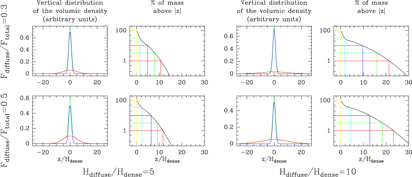
Figure 20.— First and third columns: Vertical distributions of the total volume density (green), decomposed into the sum of two Gaussian of different scale height. The broad and narrow Gaussian are respectively called diffuse (red) and dense (blue). Second and fourth columns: Percentage of the vertical mass above a given altitude in scale height unit of the dense Gaussian for the total distributions plotted in the first and third columns. The vertical lines indicate the altitudes above which 1% (red), 3% (green), 10% (blue), 33% (cyan), and 100% (yellow) of the mass is located. The ratio of the integrated masses of the diffuse over the total (diffuse+dense) are 0.3 for the top row and 0.5 for the bottom row. The two right (respectively left) columns are for a diffuse scale height 5 (respectively 10) times higher than the dense scale height. This allows us to quantify the mass of molecular gas which is extra-planar in different scenarii.

At the angular resolution of the IRAM-30m ($22.5^{\prime\prime}$), the $T(\mbox{${}^{12}$CO})/T(\mbox{${}^{13}$CO})$ increases from 6 to 11 with a typical value of $\sim$ 8 in M51. Assuming a Galactic [¹²C]/[¹³C] elemental ratio, the comparison with our Galaxy points towards the interpretation that a significant fraction of the CO emitting gas is diffuse. Is this visible in the emission of C⁺? Nikola et al. (2001) published the first map of the 158$\,\mathrm{\mu{}m}$ [Cii] emission at $55^{\prime\prime}$ resolution for M51 obtained with the Kuiper Airborne Observatory. The interpretation of this emission is difficult because it originates mostly from the warm ionized medium, though the cold neutral medium contributes significantly to the [Cii] emission. In the cold neutral medium, the density solution is degenerate, i.e., the medium could have either a low ($\sim 100-300\,\mathrm{cm^{-3}}$) or a high ($10^{3}-10^{6}\,\mathrm{cm^{-3}}$) density. They conclude that “A large fraction of the overall [Cii] emission in M51 can originate in an underlying extended medium.” A $12^{\prime\prime}$-resolution [Cii] maps was observed as part of a Herschel/PACS guaranted time project (PI: C. Wilson, Parkin et al., in prep.). The comparison of this map with the $22.5^{\prime\prime}$ decomposition between compact and extended sources (see Fig. 35) will probably shed light on the origin of the [Cii].

3.5. Discussion

Here we discuss the structure of the gas that emits the extended component — in particular the fact that it could be substructured like drops in fog — and the amount of gas that is extra-planar. We then summarize results about extra-planar gas traced in Hi and CO. We finish with a discussion of the possible origin of extra-planar CO emission.

3.5.1 Structure of the extended component

Giant molecular clouds are often thought to be composed of small clumps that are unresolved, i.e. a set of point sources. Hence, the interferometer should recover all the flux of this set of point sources and short-spacings should not be needed for extra-galactic observations. This argument is incorrect for two reasons. The first reason is that the limited sensitivity of the interferometers limits the power of deconvolution to recover the flux of point sources at low signal-to-noise ratio (See Sect. 2.3.2 and 2.3.3).

The second reason why the PdBI-only data may not recover the full flux of the source is more fundamental. We first assume that the source is a set of unresolved components filling a volume that projects onto a plane-of-sky area larger than the interferometer primary beam. If the unresolved components are typically separated by an angular distance larger than the synthesized beamwidth, the interferometer will indeed recover all the flux because the GMC is observed as a set of separated point sources. In contrast, the interferometer will filter out most of the source flux when the typical angular separation between the unresolved components is smaller than the synthesized beamwidth because the source emission appears like a flat source. Well known examples of this effect are 1) fog which appears flat while made of water drops, and 2) a XIXth century pointilliste painting which appears flat when unresolved by the eye. For this reason, it is not possible to know before the observation of large complex sources like nearby galaxies whether the short-spacings will be needed, and multi-resolution CLEAN algorithms cannot help to solve this ambiguity.

To explore this further, we speculate that the CO extended component is made of diffuse gas as found in the envelopes of giant molecular clouds. This gas would have a typical mid-plane density $\lesssim 1000\,\mathrm{cm^{-3}}$, and a temperature $\lesssim 200\,\mathrm{K}$. In such conditions, the ¹²CO (1–0) is subthermally excited. Moreover, Sect. 3.3.4 indicates that the average volume density is 1$\,\mathrm{cm^{-3}}$, implying a typical volume filling factor of 0.1%. The structure of this gas is probably filamentary, as observed in our Galaxy.

3.5.2 Vertical mass distribution and extra-planar gas

Figure 20 displays the vertical distribution of the molecular gas volume density, its decomposition into two components of different scale heights, and the percentage of mass above a given galactic height $\displaystyle\left|z\right|$. In order to sample a large fraction of the sensible parameter space, we computed 4 different cases: Two fractions of flux in the extended component (either 30 or 50%) and two scale height ratios (5 and 10) between the compact and extended components. We see that the fraction of flux in both components has a significant impact on the gas distribution close to the galatic mid-plane. However, the percentage of the total mass above a given height $z$ is only marginally affected. In contrast, doubling the ratio of the scale height doubles the galaxy height above which a given mass is located. For instance, if we assume that the smallest scale height is 40$\,\mathrm{pc}$ and a scale height ratio of 5, only 2% of the total mass is above 400$\,\mathrm{pc}$ while this proportion increases to 20% when the scale height ratio is 10. We thus estimate that between 2 and 20% of the molecular gas is extra-planar, i.e. it lies at a galactic height at least 10 times larger than the scale height of the dense molecular gas.

3.5.3 Hi thick disk

Lagging, thick Hi layers have long been detected in external galaxies (see, e.g., Boomsma et al., 2005; Barbieri et al., 2005; Oosterloo et al., 2007; Boomsma et al., 2008, in NGC 253, NGC 4559, NGC 891 and NGC 6946). The Hi gas in these galaxy halos amounts to 3-30% of the total Hi mass. For edge-on galaxies, the Hi emission extends up to 12-22$\,\mathrm{kpc}$ from the galactic mid-planes.

Miller et al. (2009) studied the prototypical face-on spiral galaxy M83. They found a spatially extended component rotating in the same sense but 40-50$\,\mathrm{km\,s^{-1}}$ more slowly in projection, with a line-of-sight velocity dispersion of $10-15\,\mathrm{km\,s^{-1}}$. The spatially extended structures are coincident with the optical spiral arms. They interpreted this component as a vertically extended disk rotating in the same sense but about 100$\,\mathrm{km\,s^{-1}}$ more slowly than the kinematically cold, thin disk. It contains 5.5% of the total Hi mass within the stellar disk of the galaxy.

3.5.4 A CO thick disk in the edge-on NGC 891 galaxy

Among the previous galaxies, NGC 891 is particularly interesting. Its characteristics are very similar to the Milky Way and Garcia-Burillo et al. (1992) found in this system the first evidence for extra-planar CO emission in an edge-on galaxy. They detected molecular emission 1-1.4$\,\mathrm{kpc}$ above the disk, wide-spread along the major axis. The associated Gaussian scale height is $\geq 600\,\mathrm{pc}$, i.e. typically 2 to 3 times larger than that deduced here for M51. This CO scale height is confirmed by a new IRAM/HERA map, which now images most of the thick disk of the galaxy (Garcia-Burillo et al., in prep.), and it is consistent with the scale height derived from the PAH emission (Rand et al., 2008).

Garcia-Burillo et al. (1992) estimate this halo emission represents less than 20% of the molecular mass in the disk. However, they also state that 40 to 60% of the thin disk emission must be in a low density component (diffuse gas) to explain the typical value (8.5) of the ratio of the ¹²CO (1–0) to ¹³CO (1–0) brightnesses. Hence, the halo molecular emission could be the tip of an independent component mixed with the dense molecular thin disk. In this case, the extended component would amount for a much larger fraction of the entire molecular gas. Indeed, in a follow-up study Sofue & Nakai (1993) mapped the molecular gas at a distance of 3.5$\,\mathrm{kpc}$ from NGC 891’s galaxy center, i.e., at the ring northern side. Using a dual Gaussian fit through the emission profile extracted perpendicular to the galaxy plane, they estimate 1) that the extended component has a typical scale height of 2.1$\,\mathrm{kpc}$ and 2) that it could account for 50% of the entire molecular gas.

3.5.5 A diffuse CO thick disk in our Galaxy?

Mapping 3 strips at constant longitude within a latitude range of $[-3.5\arcdeg,+3.5\arcdeg]$, Dame & Thaddeus (1994) detected a thick molecular disk in the inner Galaxy about 3 times as wide as that of the dense central CO layer, and comparable in width to the thin Hi layer, i.e. the height profile can be fitted with a Gaussian FWHM of $\sim 230\,\mathrm{pc}$. This data also suggests that the high latitude gas lies mainly above the spiral arms. The mass of this gas would be 15% of the total if it belongs to a distinct molecular component.

Combining $E_{\mathrm{B-V}}$ reddening, Hi absorption and ¹²CO emission measurements along many diffuse lines of sight in the Milky Way, Liszt et al. (2010) recently found that the CO luminosity per H₂ molecule for diffuse gas is standard, i.e. $X_{\mathrm{CO}}=2.0\times 10^{20}\,\mathrm{cm^{-2}/(K\,km\,s^{-1})}$. This standard value was introduced by Polk et al. (1988) to take into account the contribution of the diffuse gas to the $X_{\mathrm{CO}}$ factor. Liszt et al. (2010) and Liszt & Pety (2012) then deduced that the diffuse gas contribution to the total CO luminosity seen looking down on the Milky Way is 0.47$\,\mathrm{K\,km\,s^{-1}}$ to be compared to 0.75$\,\mathrm{K\,km\,s^{-1}}$, the result from Galactic surveys. Hence, the contribution of diffuse gas to the total CO luminosity in our Galaxy would be between 39% $(=100\times 0.47/(0.47+0.75))$ and 63% $(=100\times 0.47/0.75)$, depending on the fraction of the low brightness diffuse component that was already detected by the Galactic surveys.

The typical sensitivity of wide-field CO surveys is 1$\,\mathrm{K\,km\,s^{-1}}$. In addition, they have been mostly observed before the advent of wide bandwidth receivers/spectrometers, which were installed in current facilities from $\sim 2005$ onwards. The total velocity bandwidth of the well-known widefield Galactic CO surveys is typically only $\sim 300\,\mathrm{km\,s^{-1}}$. Finally, the extension of the diffuse component we detect in M51 is large, several hundred of parsecs. Hence, such a component in our Galaxy could have been confused with low level baselines in wide-field CO surveys.

3.5.6 Possible origin of the extra-planar CO emission

The following three scenarios are typically evoked to explain gas outside the disk (e.g. Putman et al., 2012): expelled gas from the disk via galactic fountains or chimneys, accretion from the inter-galactic medium and/or tidal debris from galaxy interactions. Except for the first scenario, it is expected that the involved component reaches very large (more than a few kpc) scale heights.

Therefore we focus in the following discussion on observational and theoretical evidence for a potential flow of dense cold material from the disk to the halo caused by massive star formation. The most extreme case to be considered might be molecular outflows driven by stellar winds or nuclear AGN, as seen, e.g., in CO in the nearby starburst galaxy M82 (Walter et al., 2002), and recently by Herschel in several nearby (U)LIRGs (Sturm et al., 2011). However, typically these phenomena are restricted to the centers of galaxies.

Evidence for dense material outside the thin disk comes from observations of distinct optical extinction features in edge-on galaxies that trace extra-planar dust. Howk (2005) summarizes the findings on extra-planar dust in nearby galaxies: extra-planar dust is found out to scale heights of $z\leq 2\,\mathrm{kpc}$, correlates well with regions of massive star formation in the disk and the total amount of star formation, and appears to reside in cold dense gas with densities of $n(\mbox{H})>25\,\mathrm{cm^{-3}}$. In this context the detection of abundant extra-planar PAH emission is interesting. Rand et al. (2011) find PAH emission out to $\sim 0.5\,-\,1\,\mathrm{kpc}$ above the disk plane in two edge-on spiral galaxies with detected extra-planar dust and detect emission from the mid-IR $17\,\mathrm{\mu{}m}$ H₂ line out to distances of 2$\,\mathrm{kpc}$ in their targets. They speculate that massive star formation in the disk is the cause for the extra-planar cold interstellar medium detected.

The resolved CO emission in M51 is preferentially found along the convex side of the spiral arms where massive star formation is ongoing and has an inferred scale height of $z\sim 200\,\mathrm{pc}$. These two findings are very similar to results of the studies of extra-planar dust and PAH emission. Thus we speculate that indeed star formation via galactic fountains or chimneys has transported some of the molecular material away from the disk.

Several simulations of disk galaxies with star formation also suggest that this explanation might be valid. The simulations have shown that cold ($T\lesssim 200\,\mathrm{K}$), dense gas can reach heights of $100-200\,\mathrm{pc}$ above the plane, but only when stellar feedback is included (Wada, 2008; Koyama & Ostriker, 2009; Dobbs et al., 2011; Acreman et al., 2012; Hill et al., 2012). Dobbs et al. (2011) find the scale height of the cold gas is $\sim 50-100\,\mathrm{pc}$, depending on the level of feedback in the simulation. From the top panel of Figure 9 of Dobbs et al. (2011), it is seen that gas at heights of a few 100 parsecs is around $10^{-25}-10^{-24}\,\mathrm{g}\,\,\mathrm{cm^{-3}}$ or $20-200\,\mbox{H${}_{2}$}\,\,\mathrm{cm^{-3}})$. Gas at these densities is not typically molecular. However, the top of Figure 14 of Dobbs et al. (2008) shows that gas which has already been dense and molecular can retain a high molecular fraction down to densities of $\sim 2\,\mbox{H${}_{2}$}\,\,\mathrm{cm^{-3}}$ before the H₂ is photodissociated. Thus the simulations indicate that a possible explanation of an extended diffuse component is that stellar feedback pushes gas out to large distances above the plane, but this gas remains molecular. The likelihood of this depends on the gravitational contribution from the stars/gas in the vertical direction, the local chemistry of H₂ formation and destruction, the effects of the stellar feedback and the surface density of the gas.

4. Summary and conclusions

We described in detail the calibration and construction of the PAWS ¹²CO (1–0) imaging of the central $\sim 10\times 6\,\mathrm{kpc}$ ($\sim 270^{\prime\prime}\times 170^{\prime\prime}$) in M51, using observations from both the PdBI and 30m telescope. The achieved spatial resolution of 40$\,\mathrm{pc}$ ($1.1^{\prime\prime}$) is close to the typical size of galactic GMCs, and at least 10 times smaller in area than previous interferometric maps obtained at OVRO, BIMA and CARMA (Aalto et al., 1999; Helfer et al., 2003; Koda et al., 2011). The median brightness sensitivity of 0.4$\,\mathrm{K}$ in 5$\,\mathrm{km\,s^{-1}}$ channel spacing corresponds to $8.6\,\mathrm{M_{\odot}}\,\,\mathrm{pc}^{-2}$. The total flux in the PAWS field of view and in a velocity range of $\pm 120\,\mathrm{km\,s^{-1}}$ around the LSR systemic velocity is 64% of the total M51 flux of $1.4\times 10^{9}\,\mathrm{K\,km\,s^{-1}\,pc^{2}}$, i.e., a molecular gas mass of $6.2\times 10^{9}\,\mathrm{M_{\odot}}$ (helium included). The mean CO integrated intensity and molecular mass surface density inside the PAWS field of view are $18\,\mathrm{K\,km\,s^{-1}}$ and $77\,\mathrm{M_{\odot}}\,\mathrm{pc}^{-2}$, respectively.

The interferometer recovers only $(50\pm 10)\%$ of the total flux. The remaining flux is mostly distributed on scales larger than 1.3$\,\mathrm{kpc}$ ($36^{\prime\prime}$). Hence, the flux is about equally distributed into a spatially extended and a spatially compact component. Using the hybrid synthesis (PdBI+30m) and the PdBI-only deconvolved results, we established that the extended component has the following properties: 1) It has a median brightness temperature of 0.14$\,\mathrm{K}$, about 18 times fainter than the compact component. 2) It covers about 30% of the PAWS field of view, about 15 times as much as the compact component. 3) Its plane-of-sky kinematics evolves smoothly, while plane-of-sky kinematics of the compact component are more affected by streaming motions. 4) Its linewidth is typically twice as large as that of the compact component. 5) Outside the region dominated by the galaxy bulge and inner nuclear bar, its typical scale height is $\sim 200\,\mathrm{pc}$, or five times the compact component scale height. 6) Its typical gas mid-plane pressure is $\sim(2-4)\times 10^{5}\,\mathrm{K\,cm^{-3}}$, in approximate pressure equilibrium with the compact component. 7) Its typical average mid-plane gas volume density is $\sim 1\mbox{H${}_{2}$}\,\,\mathrm{cm^{-3}}$, 10 times less dense than the compact component.

We estimated between 2 and 20% of the total molecular mass to be extra-planar, i.e. at galactic heights larger than 400$\,\mathrm{pc}$. We emphasized that, while the emission of the extended component is mostly structured at spatial scale larger than $36^{\prime\prime}$, it is probably made of unresolved filamentary structures, which could typically fill 0.1% of the volume of the extended component. The $T(\mbox{${}^{12}$CO})/T(\mbox{${}^{13}$CO})$ ratio at $23.6^{\prime\prime}$ resolution ranges from $\sim 7$ to $\sim 11$ when going from the inner to the outer part of the galaxy, in agreement with a mixture of dense and diffuse gas evolving from completely molecular in the inner galaxy to half atomic in the outer galaxy.

Atomic thick disks are very common. Evidence for a molecular thick disk exists in at least the edge-on NGC 891 galaxy. A thick molecular disk about 3 times as wide as the dense central CO layer was detected in the inner part of our Galaxy. We thus interpret the extended component of M51 as a diffuse CO thick disk. The underlying physical interpretation of the ¹²CO (1–0) emission is different. If the gas is dense, it fills a small fraction of the interstellar volume; it is confined by ram or turbulent pressure (if not gravitationally bound); and it is on the verge of forming stars. If the gas is diffuse, it is a warmer, low pressure medium filling a large fraction of the interstellar volume; it contributes more the mid-IR or PAH emission; and it is probably not gravitionally bound or about to form stars.

Appendix A CO luminosity and molecular gas masses

A.1. Computations

The CO luminosity, $L_{\mathrm{CO}}$, is estimated from the main beam temperature, $T_{\mathrm{mb}}$, as

$$L_{\mathrm{CO}}=\displaystyle\left\{\sum_{l,m,v}\,T_{\mathrm{mb}}(l,m,v)\right\}\,\Delta lmv,$$ (A1)

where $(l,m,v)$ are the indices of the position, position, velocity data cube and $\Delta lmv$ is the volume of one pixel of this cube computed as

$$\Delta lmv=\Delta v\,\displaystyle\left[\frac{\Delta l}{1^{\prime\prime}}\,\frac{\Delta m}{1^{\prime\prime}}\,\displaystyle\left(37\,\mathrm{pc}\frac{D}{7.6\,\mathrm{Mpc}}\right)^{2}\right].$$ (A2)

The uncertainty on this luminosity is computed as

$$\delta L_{\mathrm{CO}}=\sqrt{\sum_{l,m,v}\,\eta(l,m,v)\,\delta T_{\mathrm{mb}}^{2}(l,m,v)}\,\Delta lmv,$$ (A3)

where $\delta T_{\mathrm{mb}}(l,m,v)$ is the noise level for the pixel $(l,m,v)$ and $\eta(l,m,v)$ is the factor which reflects the correlations between pixels. If we assume that the noise level is independent of the velocity channel and that the velocity channels are uncorrelated, we obtain

$$\delta L_{\mathrm{CO}}=\sqrt{\sum_{l,m}\,n_{v}(l,m)\,\eta(l,m)\,\delta T_{\mathrm{mb}}^{2}(l,m)}\,\Delta lmv,$$ (A4)

where $n_{v}(l,m)$ is the number of velocity channels for the position (l,m). The correlation between spatial pixels can be approximated as the inverse of the number of pixels in the resolution area, i.e.,

$$\eta(l,m)=\frac{8\log(2)\Delta l\Delta m}{2\pi\Theta\theta},$$ (A5)

where $\Theta$ and $\theta$ are respectively the FWHM major and minor axes of the Gaussian beam. It is independent of the pixel position $(l,m)$.

The mass of the associated molecular gas, $M_{\mbox{H${}_{2}$}}$, is then

$$M_{\mbox{H${}_{2}$}}\pm\delta M_{\mbox{H${}_{2}$}}=X_{\mathrm{CO}}\,\displaystyle\left(L_{\mathrm{CO}}\pm\delta L_{\mathrm{CO}}\right),$$ (A6)

where $X_{\mathrm{CO}}$ is the CO-to-H₂ conversion factor. We will use the standard Galactic conversion factor

$$X_{\mathrm{CO}} = 2.0\times 10^{20}\mbox{H${}_{2}$}\,\mathrm{cm^{-2}/(K\,km\,s^{-1})}$$ (A7)

$$= 4.35\,\mathrm{M_{\odot}}\,\mathrm{pc}^{-2}/(\,\mathrm{K\,km\,s^{-1}}).$$ (A8)

The last value includes a factor of 1.36 by mass for the presence of helium.

A.2. Applications to M51

The direct sum of the pixel brightness over the field of view observed with the IRAM-30m map and between the $[-200,+300]\,\mathrm{km\,s^{-1}}$ velocity range indicates that the total CO luminosity of M51 (including the companion) is $1.442\times 10^{9}\pm 4\times 10^{5}\,\mathrm{K\,km\,s^{-1}\,pc^{2}}$. The same computation in the $[-120,+120]\,\mathrm{km\,s^{-1}}$ velocity range (where mainly M51a emits) gives $1.441\times 10^{9}\pm 3\times 10^{5}\,\mathrm{K\,km\,s^{-1}\,pc^{2}}$. Finally, the direct sum of the pixel brightness over the field of view where the line integrated emission is measured with a signal to noise ratio larger than 3 gives $1.428\times 10^{9}\pm 2\times 10^{5}\,\mathrm{K\,km\,s^{-1}\,pc^{2}}$. It is clear that the uncertainty on the result decreases when the summed volume of the cube is reduced because most of the original volume is devoid of signal. But reducing the volume introduces some kind of bias. However, the total luminosity does not vary significantly in both three results. We thus assume that most of the signal is contained within the smallest volume probed here. This in particular implies that the luminosity associated with the companion but outside the $[-120,+120]\,\mathrm{km\,s^{-1}}$ velocity range is negligible. The uncertainties are small compared to the absolute flux uncertainty ($\lesssim 10\%$, Kramer et al., 2008) and the distance uncertainty (13%). We quote them once above to show that the radiometric noise is negligible when estimating the CO luminosity. The surface where emission is detected is 38.3 square arcminutes, i.e., $1.9\times 10^{8}\,\mathrm{pc}^{2}$. The associated total mass, mean brightness, and mass surface density are respectively $6.2\times 10^{9}\,\mathrm{M_{\odot}}$, $7.6\,\mathrm{K\,km\,s^{-1}}$, and $33\,\mathrm{M_{\odot}}\,\mathrm{pc}^{-2}$. These values are summarized in Table 1.

The direct sum of the pixel brightness over the PAWS field of view and between the $[-120,+120]\,\mathrm{km\,s^{-1}}$ velocity range indicates that the final hybrid synthesis data cube contains a total CO luminosity of $9.1\times 10^{8}\,\mathrm{K\,km\,s^{-1}\,pc^{2}}$. This corresponds to a molecular gas mass of $4.0\times 10^{9}\,\mathrm{M_{\odot}}$. The total surface covered was 10.5 square arcminutes, i.e. $5.1\times 10^{7}\,\mathrm{pc}^{2}$. The mean brightness and mean surface density are respectively $18\,\mathrm{K\,km\,s^{-1}}$ and $77\,\mathrm{M_{\odot}}\,\mathrm{pc}^{-2}$.

Appendix B Masking techniques

Table 7Total CO flux measured within the PdBI+30m data cube, as measured from integrated intensity images constructed using different techniques to isolate significant emission (see text).

Method	Parameters	Total CO luminosity
		[$\times 10^{8}\,\mathrm{K\,km\,s^{-1}\,pc^{2}}$]
Direct sum	$\mathbf{[-120,+120]\,\mathrm{km\,s^{-1}}}$	9.1
Sigma-clipping	$T_{\mathrm{mb}}>1\sigma$	417
	$T_{\mathrm{mb}}>2\sigma$	16
	$\mathbf{T_{\mathrm{mb}}>3\sigma}$	7.0
	$T_{\mathrm{mb}}>4\sigma$	4.6
	$T_{\mathrm{mb}}>5\sigma$	3.5
Dilated mask	$(t,p)=(3,1.2)$	10
	$(t,p)=(3,2)$	6.9
	$(t,p)=(4,1.2)$	7.6
	$(t,p)=(4,2)$	5.8
	$\mathbf{(t,p)=(5,1.2)}$	7.2
	$(t,p)=(5,2)$	5.6
Smooth & mask	$(\theta,m)=(2.0,3)$	8.7
	$(\theta,m)=(2.0,5)$	5.6
	$(\theta,m)=(2.4,3)$	8.7
	$(\theta,m)=(2.4,5)$	6.0
	$(\theta,m)=(3.0,3)$	8.7
	$(\theta,m)=(3.0,5)$	6.4
	$(\theta,m)=(3.6,3)$	8.6
	$\mathbf{(\theta,m)=(3.6,5)}$	6.5
Hi prior	$10\,\mathrm{km\,s^{-1}}$ window	3.2
	$20\,\mathrm{km\,s^{-1}}$ window	5.0
	$\mathbf{50\,\mathrm{km\,s^{-1}}}$ window	8.0
Combined		8.5

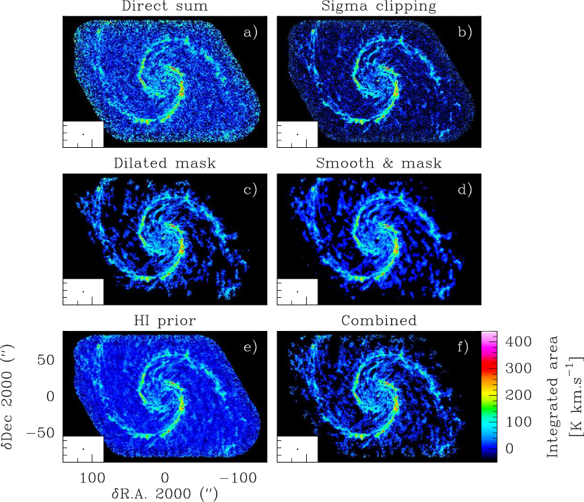
Figure 21.— Integrated intensity images constructed from the hybrid synthesis cube using different techniques: [a] direct sum of all pixels; [b] sigma-clipping method with a threshold of $5\sigma$; [c] dilated mask method with $(t,p)=(5,1.2)$; [d] smooth-and-mask method with $(\theta,m)=(3.6,5)$; [e] Hi prior method, with a 50$\,\mathrm{km\,s^{-1}}$ integration window; [f] the combined method (see text). All images are presented on the same intensity scale, which is displayed near the bottom right image.

In the previous section, we have seen that the line 0th order moment is much noisier when the velocity range used for integration includes a large number of channels devoid of signal. This effect is amplified when computing the line 1st and 2nd order moments. It is thus desirable to limit the velocity range of integration to channels where signal is detected. As the systematic motions are large for a galaxy, using a single velocity range for all the sky positions unavoidably implies moving the velocity range of integration from position to position. Defining such moving velocity ranges is never straightforward. In the case of the PAWS hybrid synthesis data set, it is even more complex because a large fraction of the flux lies at brightnesses barely detected (1 to $3\sigma$).

Moreover, masking out noisy channels always implies the risk to bias the result. We therefore explored several alternative masking methods. In order to quantify the benefit over cost of different techniques, we compare the noise and signal aspects of 0th order moments images (Fig. 21) and the total luminosity found inside the kept velocity channels (Table 7). Direct sum over a given velocity range produces an integrated intensity map that is dominated by noise (see Fig. 21[a]) because CO emission is typically only detected in a few velocity channels along each line-of-sight. But it produces a robust estimate for the total CO luminosity.

The first alternative we tried is a simple sigma-clipping method, whereby pixels containing emission with low significance were excluded. We tested various brightness thresholds between 1 and 5$\sigma$, where $\sigma$ is the standard deviation of the noise fluctuations estimated using $\sim 25$ emission-free channels for each line-of-sight. The integrated intensity images were constructed by summing all unmasked (i.e. ‘good’) pixels across the observed LSR velocity range, i.e. $[-297.5,+297.5]$$\,\mathrm{km\,s^{-1}}$. As expected, lower thresholds produce maps that are dominated by noise peaks, especially in the interarm region. Higher thresholds produce maps with a cleaner appearance, but also do a poorer job of recovering the total luminosity (see Table 7). For thresholds above $\sim 3\sigma$, it is evident that genuine low surface brightness emission in the interarm region is omitted. A map constructed using a $3\sigma$ threshold is shown as an example in Fig. 21[b].

For the second method, which we call the dilated mask method, we defined islands of significant emission in the hybrid synthesis data cube by selecting peaks above a threshold of $t\sigma$ across two contiguous velocity channels. This preliminary mask was expanded to include all connected pixels with emission greater than $p\sigma$. Several combinations of $t$ and $p$ values were tested, using $t\in[3,7]$ and $p\in[1.2,3]$. The final mask was then applied to the original data cube, and the integrated intensity image was constructed by summing unmasked pixels within the LSR velocity range $[-297.5,+297.5]$$\,\mathrm{km\,s^{-1}}$. We consider the map obtained for $(t,p)=(5,1.2)$, shown in Fig. 21[c], as the best map produced using this method. Higher $t$ values tended to omit genuine low surface brightness emission, whereas lower $t$ values include a larger number of spurious noise peaks, especially in the interarm region and at the edges of the survey field. Setting $p=1.2$ produced optimal results in the sense that faint emission around the edge of bright structures is retained within the mask, but the algorithm does not misidentify large patches of noise as genuine emission. The total CO luminosity within the map shown in Fig. 21[c] is only $7.6\times 10^{8}$ $\,\mathrm{K\,km\,s^{-1}\,pc^{2}}$, however, indicating that a significant fraction of the CO emission within the survey field is not recovered in this image.

For the third method, which we call the smooth-and-mask method (e.g. Helfer et al., 2003), we generated a mask by convolving the original hybrid synthesis cube to a coarser spatial resolution using a Gaussian smoothing kernel with FWHM $\theta$. The RMS noise for each sightline within the smoothed cube was estimated from $\sim 25$ emission-free channels, then pixels in the smoothed cube with emission below a significance threshold $m\sigma$ were blanked. After transferring this mask back to the original data cube, the integrated intensity image was constructed by summing unmasked pixels across the LSR velocity range $[-297.5,+297.5]$$\,\mathrm{km\,s^{-1}}$. As for the previous methods, we experimented with different combinations of the $\theta$ and $m$ parameters. We consider the map obtained using a 3$\farcs$6 kernel and a $5\sigma$ threshold to be the best produced using this method. The total CO luminosity within this map, which is shown in Fig. 21[d], is $6.9\times 10^{8}$ $\,\mathrm{K\,km\,s^{-1}\,pc^{2}}$.

For the fourth method, we integrated the PdBI+30m data cube over a narrow velocity range (which we refer to as the ‘integration window’), centered on the radial velocity at the peak of the Hi line profile for each line-of-sight. We call this method the ‘Hi prior method’. The Hi velocity template was constructed using the Hi data cube from THINGS (Walter et al., 2008), which covers the entire disk of M51 at $\sim 11\arcsec$ resolution. Integration windows with velocity widths between 10 and 100$\,\mathrm{km\,s^{-1}}$ were tested. The rationale behind this approach is that CO emission in nearby galaxies is mostly associated with high brightness Hi emission (e.g. Schruba et al., 2011; Engargiola et al., 2003). Comparison with maps in the other panels of Fig. 21 suggests that CO emission in the nuclear region of M51 is not well-recovered by this method. One advantage of this approach, however, is that it yields an upper limit on the CO integrated intensity for pixels without detectable emission, and may therefore be more suitable for some types of quantitative analysis. The map for a 50 $\,\mathrm{km\,s^{-1}}$ integration window is shown in Fig. 21[e]. The total luminosity in this map is $8.4\times 10^{8}$ $\,\mathrm{K\,km\,s^{-1}\,pc^{2}}$.

Finally, we used the strengths of two of these methods to build our best mask. We started by building two 2D masks based on the second (dilated mask) and fourth (Hi prior) approaches. In each case, we constructed a 3D dilated mask from the hybrid synthesis datacube. However, this technique also catches noise patches at “wrong” velocities. To remove these, we computed the associated centroid velocity map, and we then produced a 2D mask where the CO velocity centroids differed by less than 30$\,\mathrm{km\,s^{-1}}$ from a map of the Hi velocity field. Using this 2D mask, we could build a 3D filtered mask.

The difference between these two 3D filtered masks comes from the different thresholds used to produce initial 3D dilated masks. The first dilated mask used $(t,p)=(4,1)$, which allows us to find isolated faint point sources. However, these parameters also catches isolated noise at “forbidden” velocities, which will considerably bias the line-of-sight CO centroid velocities. The comparison of the CO and HI centroid velocities may thus kill perfectly valid lines of sight. This happens in particular in the M51 central part. To avoid this effects, the second dilated mask used $(t,p)=(10,1.5)$. The high signal-to-noise ratio (10) starting point ensures that no outlier velocities will be caught in the 3D mask but it will miss isolated low brightness signal. The two 3d filtered masks thus identify complementary kind of signal. We finally make the union of these 3D filtered masks to obtain the final mask. The resulting 0-moment map, which has a total luminosity of $8.5\times 10^{8}\,\mathrm{K\,km\,s^{-1}\,pc^{2}}$, is shown in Fig. 21[f]. This map contains 93% of the total luminosity computed from direct summation. The comparison of these maps with the ones of the other methods shows that it is the most successful at recovering all genuine emission within the data cube. This mask was thus used to compute the 1st and 2nd order moments of the hybrid synthesis cube at $1^{\prime\prime}$ resolution.

Appendix C Modeling the impact of the IRAM-30m error beam

In this appendix, we assess how much the error beams of the IRAM-30m contribute to the extended emission. To do this, we first convolved a model of the source emission in the PAWS field of view 1) with the ideal 30m beam and 2) with a model of the true 30m beam, including the diffraction pattern and the error beams. We then subtracted the convolved maps to estimate the contribution of the diffraction pattern and error beams to the extended emission. We first describe the 30m beam and the source models used, before discussing the results.

C.1. Beam model

Table 8Parameters used to model the IRAM-30m beam at 115.271202$\,\mathrm{GHz}$. Adapted from Greve et al. (1998).

	Main beam	1st error beam	2nd error beam	3rd error beam
Origin	Diffraction	Large scale	Panel Frame	Panel
	pattern	deformations	misalignments	deformations
Correlation length	—	$2.5-3.5\,\mathrm{m}$	$1.5-2.0\,\mathrm{m}$	$0.3-0.5\,\mathrm{m}$
Surface rms	—	$\lesssim 0.06\,\mathrm{mm}$	$0.055\,\mathrm{mm}$	$0.055\,\mathrm{mm}$
Beamwidth (FWHM)	$21.3^{\prime\prime}$	$230^{\prime\prime}$	$330^{\prime\prime}$	$1840^{\prime\prime}$
Power amplitude	1.00	$9.0\times 10^{-4}$	$2.7\times 10^{-4}$	$3.1\times 10^{-5}$
Relative power	71.8%	7.4%	4.7%	16.1%

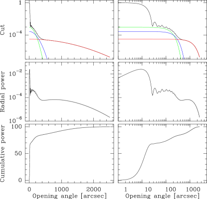
Figure 22.— Characteristics of the IRAM-30m beam at the frequency of the ¹²CO (1–0) line as a function of the opening angle in linear (left column) and logarithmic (right column) scales. Top: Cut of the beam profile, normalized to unity at $\theta=0^{\prime\prime}$. The black curve is a combination of the diffraction pattern and the three Gaussian error beams. The green, blue, and red curves displays the three error beams. Middle: Beam power contained in circular annuli, normalized so that the integral is unity. Bottom: Beam power integrated over the solid angle sustained by the opening angle, normalized to 100%.

After measuring the 30m beam pattern at 3.4, 2, 1.3 and 0.8$\,\mathrm{mm}$ from total power scans across the Moon around full Moon and new Moon, Greve et al. (1998) modelled the beam using antenna tolerance theory. They deduced that the beam consists of the diffracted beam, two underlying error beams, which can be explained by the panel dimensions, and a beam deformation mostly due to large-scale transient residual deformations of the telescope structure. We scaled their results to the frequency of the ¹²CO (1–0) line to model the error beams we use. The diffraction pattern was computed for an antenna illuminated by a Gaussian beam of 12.5 dB edge taper and a ratio of the secondary-to-primary diameter (blockage factor) of 0.067, using the prescription of Goldsmith (1998). Figure 22 shows the properties of the resulting beam and Table 8 lists the typical scales, amplitudes, and contributions to the total power of the different beam components.

The diffraction pattern and two of the three error beams are linked to the structure of the primary mirror of the 30m, which have not changed since the study of Greve et al. (1998). Hence the typical angular scales of the different error beams stay constant over time. However, the 30m primary surface accuracy improved in 2000 after several holography campaigns. Moreover, the thermal balance of the telescope primary surface was also improved around this time. Both effects explain why the beam efficiencies of the 30m are significantly higher today than the values provided by Greve et al. (1998): e.g., 0.78 instead of 0.72 at the ¹²CO (1–0) frequency. We used slightly different values of the 30m beam efficiency in our analysis for historical reason. As no newer detailed measurements of the error beams are available, we used 0.72 for consistency with the work by Greve et al. (1998) to model the beam here, while we applied 0.75 to the data. As the current best estimate of the beam efficiency is 0.78, both values present only variations of a few percent and do not alter our conclusions. In particular, our estimates of the error beam contribution can be seen as a firm upper limit.

C.2. Source model

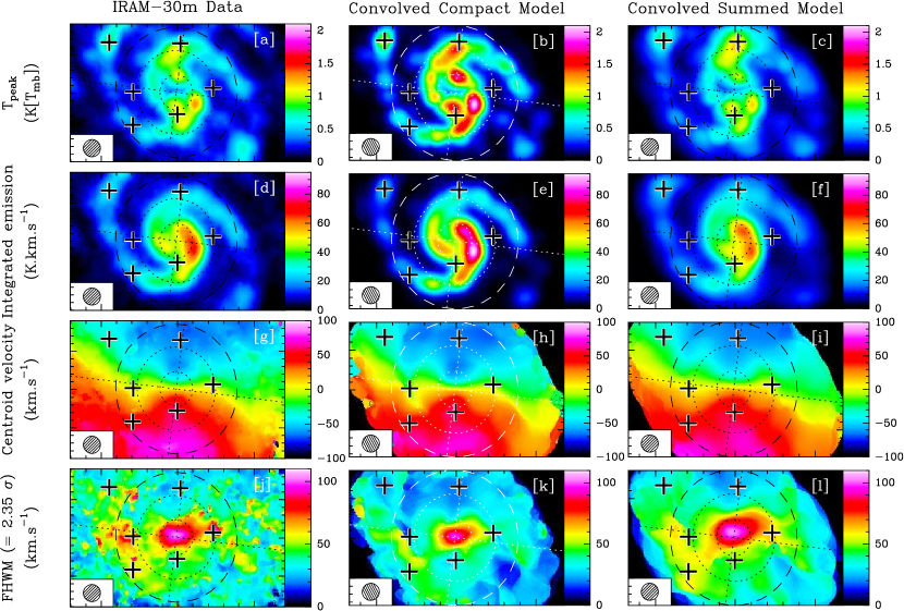
Figure 23.— Comparison of the spatial distribution (from top to bottom) of the peak intensity, integrated intensity, centroid velocity, and the line full width at half maximum (i.e., 2.35 times the standard deviation in velocity) of the ¹²CO (1–0) emission from the actual observations (left column), and the two models convolved with the modeled 30m beam (middle and right column). The angular resolution is indicated by a circle in the bottom left corner of each panel. The intensity scale is shown on the right-hand side of each panel. The 3 images of each row share the same intensity scale to facilitate a meaningful visual comparison. The crosses on the images show the positions of the spectra displayed in Fig. 24. Other plot annotations are the same as in Fig. 13.

The best proxy for the source model is the result of this project, i.e. the distribution of the emission measured in the PAWS field of view. We made two different source models. First, we want to check whether the error beam contribution of the compact sources alone can account for the extended emission. We started with the $1^{\prime\prime}$ PdBI-only data cube, and we set to zero all pixels whose brightness was below 3 times the noise level in order to avoid spurious sources. We multiplied all pixel brightnesses by a factor of about 2, needed to recover the total flux in the PAWS field of view. This assumes that all extended emission is spurious and that any flux associated with it should indeed belong to compact sources. We will refer to this cube as the compact model.

In contrast, we assume for the second model that the extended emission is genuine. To model the extended component, we start with the $6^{\prime\prime}$ subtracted cube, in which we set to zero all pixels whose brightness was below 3 times the noise level. We then added all the brightness of the $1^{\prime\prime}$ PdBI-only data cube whose brightness is above 3 times the noise level. The flux contained in this model is then 3% larger than the flux measured in the PAWS field of view. We will refer to this cube as the summed model.

C.3. Modeling results

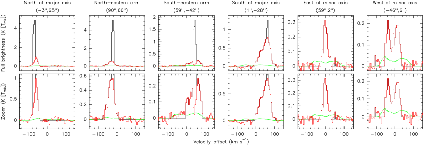
Figure 24.— Comparison of the spectra of our summed model (in black), the extended emission as measured in the $6^{\prime\prime}$ subtracted cube (in red), and the error beam contribution (in green), at six positions where the extended emission shows different characteristics. These positions are displayed as crosses on the images of the extended emission moments in Fig. 13. The bottom row shows a brightness zoom of the top row.

We convolved each model with the true 30m beam model. We normalized the result by the main beam efficiency to get to the main beam temperature scale. Fig. 23 compares the moments of both modeled 30m emission with the measured emission. All the moments were computed using the same position-position-velocity mask (the one of the data) to ensure a meaningful comparison. The compact model produces much higher peak temperatures and integrated emission in the arms, while it understimates the flux in the inter-arm region. The summed model provides a much better match to the observations.

We subtracted from the previous cubes the associated brightness model convolved with the ideal 30m beam. This yields the contribution of the error beams to the signal measured with the 30m. In particular, it allows us to estimate the error beam contribution to the extended emission, as we showed in Section 3.1.4 that the flux of the extended emission is mostly structured at scales larger than $36^{\prime\prime}$, i.e. at scales larger than the ideal 30m beam FWHM. For both source models, the flux scattered into the error beams is less than 20% the total flux in the PAWS field of view but the peak brightness due to the error beam contribution is only 55$\,\mathrm{mK}$, i.e., about 3.5 times the median noise level of the 30m observations. The typical angular scales of the error beams are large, implying that the flux is scattered at low brightness level over wide regions of the sky. The median value of the error beam contribution is 19$\,\mathrm{mK}$, while pixels brighter than 5 times the noise level have a median of 140$\,\mathrm{mK}$ in the extended emission measured at $6^{\prime\prime}$ (see Sect. 3.2.1). Moreover, flux above 0.1$\,\mathrm{K}$ in the extended emission cube represents 79% of the flux in this cube (we subtracted the flux contributed by the error beams in the same mask to compute this value). We deduce that the error beams contribute less than 20% of the flux in the extended emission, i.e., less than 10% of the total flux in the PAWS field of view. We speculate that the baselining of the 30m spectra removed a large fraction of the flux associated with the error beams.

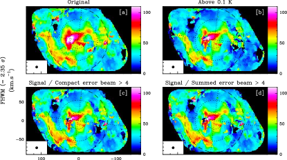
Figure 25.— Comparison of the spatial distribution of the line full width at half maximum (i.e., 2.35 times the standard deviation in velocity) of the ¹²CO (1–0) extended emission measured at $6^{\prime\prime}$. Different masking techniques were used to test the impact of the error beams on the computation of the line width (see text). The angular resolution is indicated by a circle in the bottom left corner of each panel. The intensity scale is shown on the right-hand side of each panel. The images share the same intensity scale to facilitate comparison. The major and minor axes are displayed as perpendicular dotted lines. The dotted circles show the two inner corotation resonances at radii equal to $23^{\prime\prime}$ and $55^{\prime\prime}$, while the dashed circle shows the start of the material arms at a radius equal to $85^{\prime\prime}$ (Meidt et al., 2013).

Fig. 24 compares the spectra of our summed model, the extended emission, and the contribution from the error beams at six positions, which sample different ratios of compact to extended brightness as well as different characteristics of the extended emission. These spectra illustrate that the emission associated with the error beams has a very different signature in space and velocity from the extended emission distribution. In particular, the spectra resulting from the error beams have much wider linewidths than the observed spectra of the extended emission. We finally investigate the impact of the error beams on the moments of the extended emission. We recomputed the moments of the $6^{\prime\prime}$ extended emission cube in two different ways. First, we only include the pixels brighter than two times the peak brightness (i.e., 0.1$\,\mathrm{K}$) due to the error beams. In the second test, we include only the pixels brighter than four times the contribution of the error beam for each source model. The three resulting moment maps are similar to the original one. This is also true for the second moment or linewidth displayed in Fig. 25. We thus conclude that the large linewidths of the extended emission are genuine.

Appendix D Estimating the vertical velocity dispersion

The velocity of a parcel of gas in the galaxy frame is

$$\mathbf{v_{\mathrm{gal}}}=(\mathbf{v_{p}},\mathbf{v_{z}}),$$ (D1)

where ($\mathbf{v_{p}}$,$\mathbf{v_{z}}$) respectively are the in-plane and perpendicular to the galactic plane velocity components. In the observing frame, the Doppler effect allows us to infer an observed velocity, $v_{\mathrm{obs}}$, which is the projection of $\mathbf{v_{\mathrm{gal}}}$ along the line of sight. If $u_{p}$ is the projection of $\mathbf{v_{p}}$ on the galaxy major axis and $i$ is the inclination of the galaxy plane onto the line of sight, we get

$$v_{\mathrm{obs}}=u_{p}\,\sin i+v_{z}\,\cos i.$$ (D2)

In the optically thin limit, a line is an histogram of all the $v_{\mathrm{obs}}$ values along each line of sight. For a resolved perfectly face-on galaxy,

$$v_{\mathrm{obs}}=v_{z}.$$ (D3)

The centroid velocity would thus be constant and the linewidth would give the dispersion of the velocity distribution along the vertical axis under the condition that the velocity has a symmetric distribution of velocity along any line of sight. For a resolved edge-on galaxy,

$$v_{\mathrm{obs}}=u_{p}.$$ (D4)

If the velocity is only rotational and the density is much higher in the spiral arm, the centroid velocity is then biased towards the velocities in the spiral arm and the velocity dispersion gives an idea of the velocity content along the line of sight. This is why we still have some information about the rotation curve of the galaxy.

For any other inclination, the centroid velocity, $v_{\mathrm{cent}}$, is

$$v_{\mathrm{cent}}=\displaystyle\left<v_{\mathrm{obs}}\right>=\displaystyle\left<u_{p}\right>\,\sin i,$$ (D5)

as long as the galaxy disk is not warped and the distribution of the velocity perpendicular to the galactic plane is symmetric, i.e. $\displaystyle\left<v_{z}\right>=0$. Now, the velocity dispersion is computed as

$$\left<\displaystyle\left(v_{\mathrm{obs}}-v_{\mathrm{cent}}\right)^{2}\right>=\displaystyle\left<\displaystyle\left[v_{z}\,\cos i+\displaystyle\left(u_{p}-\displaystyle\left<u_{p}\right>\right)\,\sin i\right]^{2}\right>.$$ (D6)

Assuming that there are no correlations between vertical and horizontal motion, we obtain

$$\left<\displaystyle\left(v_{\mathrm{obs}}-v_{\mathrm{cent}}\right)^{2}\right>=\displaystyle\left<v_{z}^{2}\right>\,\cos^{2}i+\displaystyle\left<\displaystyle\left(u_{p}-\displaystyle\left<u_{p}\right>\right)^{2}\right>\,\sin^{2}i.$$ (D7)

If we also assume that the velocity field is only made of a systematic motion ($u_{\mathrm{sys}}$) parallel to the galaxy plane plus an isotropic 3D turbulent motion of typical dispersion ($\sigma_{\mathrm{turb}}$), then

$$\left<v_{z}^{2}\right>=\sigma_{\mathrm{turb}}^{2}\quad\mbox{and}$$ (D8)

$$\left<\displaystyle\left(u_{p}-\displaystyle\left<u_{p}\right>\right)^{2}\right>=\sigma_{\mathrm{turb}}^{2}+\displaystyle\left<\displaystyle\left(u_{\mathrm{sys}}-\displaystyle\left<u_{\mathrm{sys}}\right>\right)^{2}\right>.$$ (D9)

Note that $\displaystyle\left<u_{\mathrm{sys}}\right>=\displaystyle\left<u_{p}\right>$ and the turbulent component yield only one time $\sigma_{\mathrm{turb}}$ because $u_{p}$ is an unidimensional velocity component. Hence,

$$\left<\displaystyle\left(v_{\mathrm{obs}}-v_{\mathrm{cent}}\right)^{2}\right>=\sigma_{\mathrm{turb}}^{2}+\displaystyle\left<\displaystyle\left[\displaystyle\left(u_{\mathrm{sys}}-\displaystyle\left<u_{\mathrm{sys}}\right>\right)\,\sin i\right]^{2}\right>,$$ (D10)

where $\displaystyle\left<\displaystyle\left[\displaystyle\left(u_{\mathrm{sys}}-\displaystyle\left<u_{\mathrm{sys}}\right>\,\sin i\right)\right]^{2}\right>$ is the contribution of the systematic in-plane motions inside the beam to the line 2nd order moment. We can estimate this contribution as

$$\left<\displaystyle\left[\displaystyle\left(u_{\mathrm{sys}}-\displaystyle\left<u_{\mathrm{sys}}\right>\right)\,\sin i\right]^{2}\right>\sim\displaystyle\left[\displaystyle\left|\mathbf{\mathrm{grad}(v_{\mathrm{cent}}{})}\right|{}\,\frac{\theta}{\sqrt{8\ln 2}}\right]^{2},$$ (D11)

where $\theta$ is the resolution beamwidth of the observations and $\displaystyle\left|\mathbf{\mathrm{grad}(v_{\mathrm{cent}}{})}\right|$ is the modulus of the centroid velocity 2D-gradient. In our case, these last two quantities can be measured. This thus yields an estimation of the galaxy vertical velocity dispersion as the square root of

$$\left<v_{z}^{2}\right>=\sigma_{\mathrm{turb}}^{2}\sim\displaystyle\left<\displaystyle\left(v_{\mathrm{obs}}-v_{\mathrm{cent}}\right)^{2}\right>-\displaystyle\left[\displaystyle\left|\mathbf{\mathrm{grad}(v_{\mathrm{cent}}{})}\right|{}\,\frac{\theta}{2.35}\right]^{2}.$$ (D12)

Appendix E Additional material

This section displays additional material that completes the description of the observations and the presentation of the data cubes. All these tables and figures are only made available online.

Table 9 presents the weather conditions during the IRAM-30m observing run. Table 10 exhaustively lists the interferometric sessions observed during the IRAM large program PAWS. Table 11 gives the evolution of the calibrator fluxes as a function of time, a key intermediate in the absolute amplitude calibration of the data.

Figures 26 and 27 present the channel maps of the IRAM-30m single-dish data for the ¹²CO and ¹³CO (1–0) lines. Figures 28 and 28 show the channel maps of the hybrid synthesis data cube at $1^{\prime\prime}$ angular resolution, the main data product of the PAWS large program. Figures 30 and 31 overlay the channel maps of the bright compact emission as contours over the channel maps of the faint extended emission displayed in color.

Finally, Figures 32, 33, 34, and 35 summarize the properties of the decomposition of the hybrid synthesis emission into the PdBI-only and the subtracted emissions, respectively at 1, 3, 6, and $22.5^{\prime\prime}$.

Table 9Detailed parameters for the IRAM-30m observations

Observing date	Timea	$T_{\mathrm{sys}}$b	Water vapor
	hours	K [$T_{\mathrm{A}}^{*}$]	mm
18/05/2010	3.8/8.0	279	4.3-8.8
19/05/2010	2.9/8.0	275	3.6-6.1
20/05/2010	3.4/8.0	273	2.6-8.5
21/05/2010	3.6/9.0	287	5.8-9.0
22/05/2010	3.6/8.0	297	6.5-9.4

^a Two values are given for the integration time: the on-source time and the telescope time.
^b The $T_{\mathrm{sys}}$ values are given for the ¹²CO (1–0) frequency.

Table 10Detailed parameters for the PdBI observations.

Config.	$N_{\mathrm{ant}}$	Mosaic	Int. Timea	$T_{\mathrm{sys}}$	Seeing	Obs. date
		#	hours	K	arcsec
D	5	Top	2.0/09.5	150-400	1.70	29 Aug. 2009
	5	Bot	2.2/09.5	200-400	1.70	02 Oct. 2009
C	6	Top	4.3/09.5	180-250	0.68	27 Oct. 2009
	6	Bot	3.3/08.5	180-300	0.85	28 Oct. 2009
B	6	Top	1.8/08.0	200-250	0.37	20 Feb. 2010
	6	Top	1.2/05.0	200-250	0.60	02 Mar. 2010
	6	Top	1.5/05.0	160-230	0.50	04 Mar. 2010
	6	Top	3.3/07.5	180-280	0.29	11 Mar. 2010
	6	Bot	5.1/11.0	150-250	0.34	08 Mar. 2010
	6	Bot	4.2/11.5	200-300	0.50	09 Mar. 2010
	6	Bot	4.6/09.0	160-220	0.30	12 Mar. 2010
A	6	Top	1.3/03.0	180-200	0.32	14 Dec. 2009
	6	Top	3.0/08.5	180-220	0.28	17 Dec. 2009
	6	Top	5.2/11.0	160-230	0.15	18 Jan. 2010
	6	Top	2.2/05.0	200-600	0.27	22 Jan. 2010
	6	Top	3.6/07.5	180-230	0.27	12 Feb. 2010
	6	Top	1.5/04.5	160-230	0.16	13 Feb. 2010
	6	Bot	3.2/05.5	170-220	0.31	15 Dec. 2009
	6	Bot	1.5/07.5	180-400	0.35	03 Jan. 2010
	6	Bot	3.0/08.5	180-400	0.44	05 Jan. 2010
	6	Bot	3.2/05.5	180-230	0.18	23 Jan. 2010
	6	Bot	2.3/06.5	250-300	0.41	29 Jan. 2010

^a Two values are given for the integration time: the good on-source time (as if observed with 6 antennas) and the telescope time.

Table 11Flux (in Jy) of the amplitude and phase calibrators used during the PdBI calibration.

Date	1418$+$546	1308$+$326	J1332$+$473
29-aug-2009	1.05	—	0.46
02-oct-2009	1.10	2.58	—
27-oct-2009	1.06	—	0.22
28-oct-2009	1.02	2.58	—
14-dec-2009	1.11	—	0.22
15-dec-2009	1.10	2.02	—
17-dec-2009	1.16	—	0.21
03-jan-2010	1.23	2.26	—
05-jan-2010	1.23	2.16	—
18-jan-2010	1.22	—	0.23
22-jan-2010	1.16	—	0.24
23-jan-2010	1.16	1.93	—
25-jan-2010	1.22	1.83	—
29-jan-2010	1.06	1.83	—
12-feb-2010	0.98	1.91	0.22
13-feb-2010	1.00	—	0.22
20-feb-2010	0.92	—	0.18
02-mar-2010	0.92	—	0.19
04-mar-2010	0.94	—	0.20
08-mar-2010	0.94	1.92	—
09-mar-2010	0.96	1.95	—
11-mar-2010	0.96	—	—
12-mar-2010	0.96	—	—

Figure 26.— Channel maps of the ¹²CO (1–0) emission obtained with the IRAM-30m telescope. The velocity in $\,\mathrm{km\,s^{-1}}$ of each channel is displayed in the top left corner of each panel. The intensity scale (in $T_{\mathrm{mb}}$) is shared by all the panels and it is displayed in the bottom right corner of the figure. The major and minor axes are displayed as perpendicular dotted lines. The dotted circles show the two inner corotation resonances at radii equal to $23^{\prime\prime}$ and $55^{\prime\prime}$, while the dashed circle shows the start of the material arms at a radius equal to $85^{\prime\prime}$ (Meidt et al., 2013).

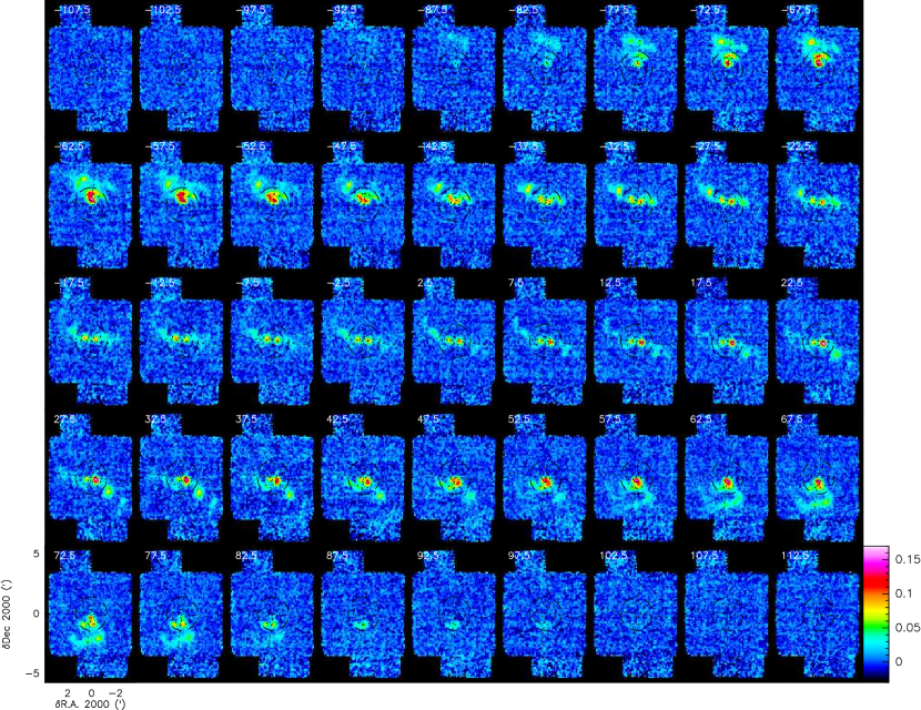
Figure 27.— Channel maps of the ¹³CO (1–0) emission obtained with the IRAM-30m telescope. The figure layout is the same as for Fig. 26.

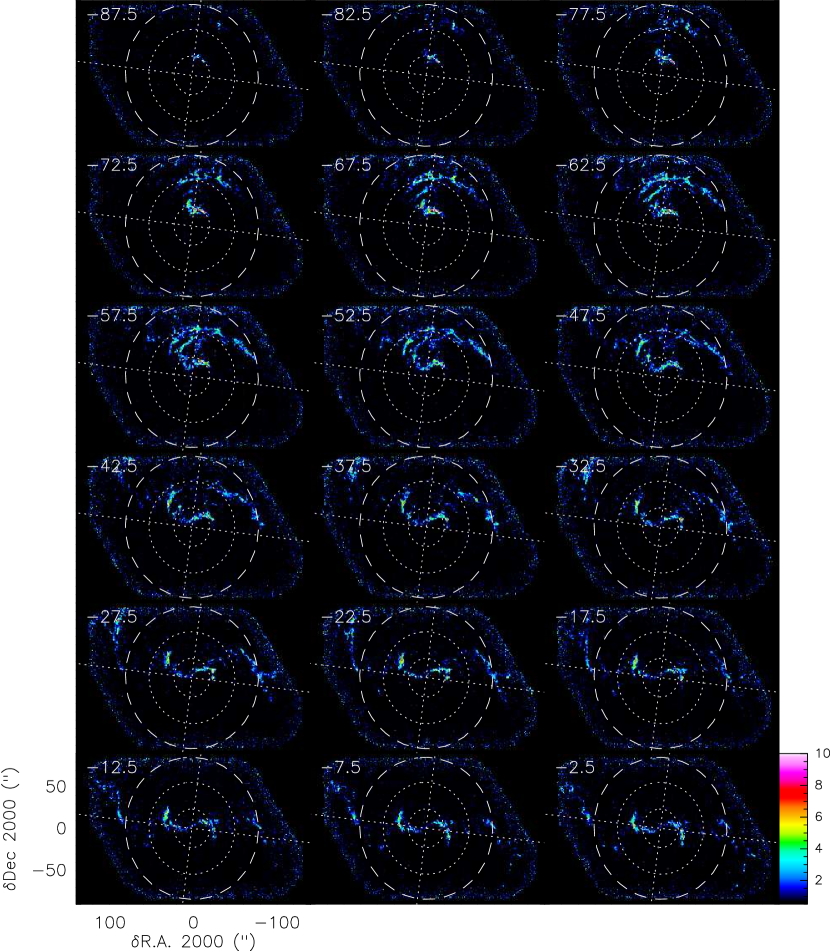
Figure 28.— Channel maps of the ¹²CO (1–0) emission obtained from the combination of IRAM-30m and IRAM-PdBI observations. The velocity of each channel in $\,\mathrm{km\,s^{-1}}$ is displayed in the top left corner of each panel. Only the negative velocity channels are shown here. The intensity scale (in $T_{\mathrm{mb}}$) is shared by all the panels and it is displayed in the bottom right corner of the figure. This intensity scale is saturated to emphasize the pixels with significant emission. The major and minor axes are displayed as perpendicular dotted lines. The dotted circles show the two inner corotation resonances at radii equal to $23^{\prime\prime}$ and $55^{\prime\prime}$, while the dashed circle shows the start of the material arms at a radius equal to $85^{\prime\prime}$ (Meidt et al., 2013).

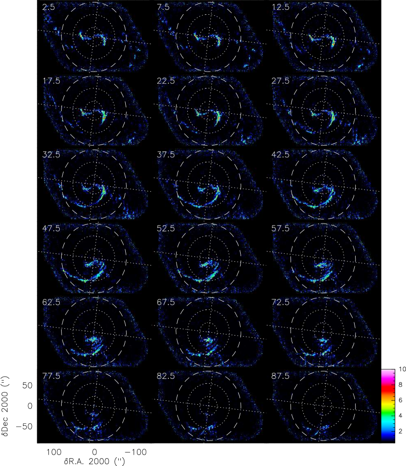
Figure 29.— Same as Fig. 28 but for the positive velocity channels.

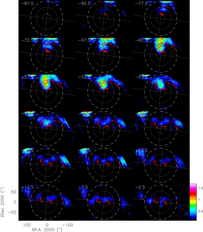
Figure 30.— Contours of the channel maps of the signal-to-noise ratio of the combined PdBI+30m cube laid over the channel maps of the resolved emission. The contour levels start at a signel-to-noise ratio of 8. The figure layout is as in Fig. 28.

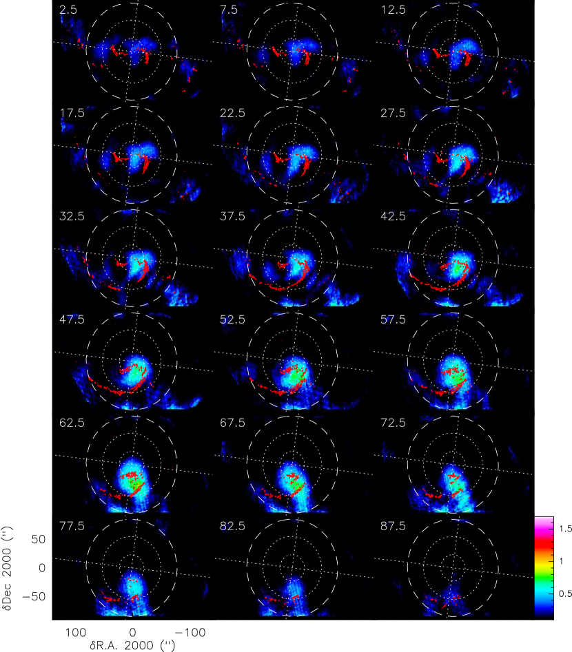
Figure 31.— Same as Fig. 30 but for the positive velocity channels.

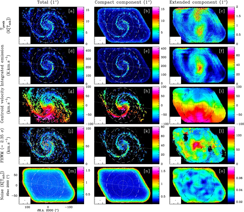
Figure 32.— Comparison of the spatial distribution at $\sim 1^{\prime\prime}$-resolution (from top to bottom) of the peak intensity, integrated intensity, centroid velocity, the line full width at half maximum (i.e., 2.35 times the standard deviation in velocity) and, rms noise of the ¹²CO (1–0) emission for the hybrid synthesis (PdBI + 30m, left column), the PdBI-only (middle column) and the subtraction of the PdBI-only from the hybrid synthesis cubes (right column). The angular resolution is shown as a circle in the bottom left corner of each panel. The intensity scale is shown on the right of each panel. The major and minor axes are displayed as perpendicular dotted lines. The dotted circles show the two inner corotation resonances at radii equal to $23^{\prime\prime}$ and $55^{\prime\prime}$, while the dashed circle shows the start of the material arms at a radius equal to $85^{\prime\prime}$ (Meidt et al., 2013).

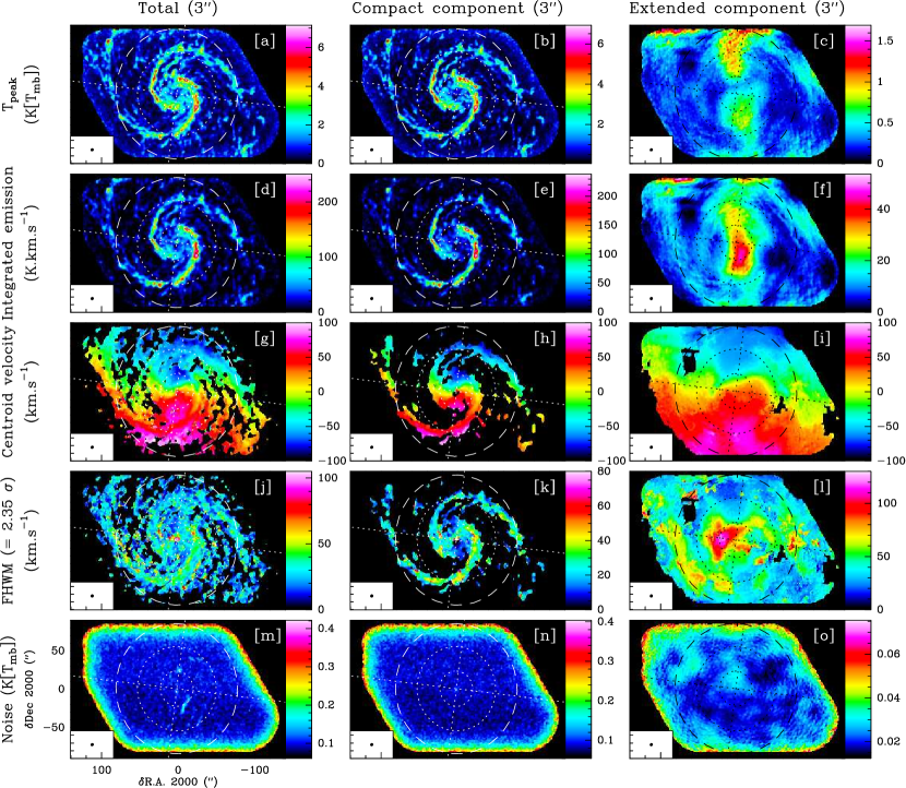
Figure 33.— Same as Fig. 32 but the comparison is done here at an angular resolution of $3^{\prime\prime}$.

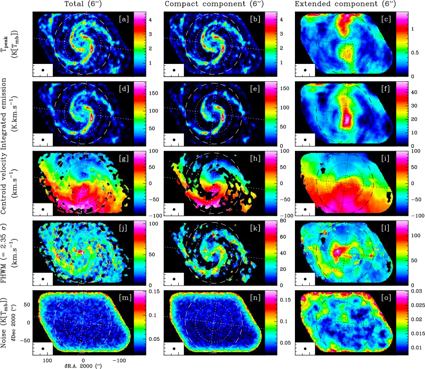
Figure 34.— Same as Fig. 32 but the comparison is done here at an angular resolution of $6^{\prime\prime}$.

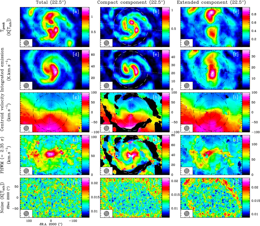
Figure 35.— Comparison of the spatial distributions at $22.5^{\prime\prime}$-resolution of the peak intensity (top), integrated intensity, centroid velocity, 2.35 times the standard deviation and rms noise (bottom) of the ¹²CO (1–0) emission for IRAM-30m cube (left column), the $6^{\prime\prime}$ PdBI-only data cube smoothed at $22.5^{\prime\prime}$ (right column), and the subtraction of the two previous cubes (middle column). The angular resolution is displayed as a circle in the bottom left corner of each panel. The intensity scale is shown on the right side of each panel. The major and minor axes are displayed as perpendicular dotted lines. The dotted circles show the two inner corotation resonances at radii equal to $23^{\prime\prime}$ and $55^{\prime\prime}$, while the dashed circle shows the start of the material arms at a radius equal to $85^{\prime\prime}$ (Meidt et al., 2013).

References

- Aalto et al. (1999) Aalto, S., Hüttemeister, S., Scoville, N. Z., & Thaddeus, P. 1999, ApJ, 522, 165
- Acreman et al. (2012) Acreman, D. M., Dobbs, C. L., Brunt, C. M., & Douglas, K. A. 2012, MNRAS, 422, 241
- Barbieri et al. (2005) Barbieri, C. V., Fraternali, F., Oosterloo, T., Bertin, G., Boomsma, R., & Sancisi, R. 2005, A&A, 439, 947
- Binney et al. (1991) Binney, J., Gerhard, O. E., Stark, A. A., Bally, J., & Uchida, K. I. 1991, MNRAS, 252, 210
- Blitz et al. (2007) Blitz, L., Fukui, Y., Kawamura, A., Leroy, A., Mizuno, N., & Rosolowsky, E. 2007, Protostars and Planets V, 81
- Blitz & Rosolowsky (2006) Blitz, L. & Rosolowsky, E. 2006, ApJ, 650, 933
- Boissier et al. (2003) Boissier, S., Prantzos, N., Boselli, A., & Gavazzi, G. 2003, MNRAS, 346, 1215
- Boomsma et al. (2005) Boomsma, R., Oosterloo, T. A., Fraternali, F., van der Hulst, J. M., & Sancisi, R. 2005, A&A, 431, 65
- Boomsma et al. (2008) —. 2008, A&A, 490, 555
- Bottema (1993) Bottema, R. 1993, A&A, 275, 16
- Bracewell (2000) Bracewell, R. N. 2000, The Fourier Transform and its Applications, 3rd edn. (McGraw-Hill)
- Ciardullo et al. (2002) Ciardullo, R., Feldmeier, J. J., Jacoby, G. H., Kuzio de Naray, R., Laychak, M. B., & Durrell, P. R. 2002, ApJ, 577, 31
- Colombo et al. (2013a) Colombo, D., Co-author, F., & Co-author, S. 2013a, ApJ
- Colombo et al. (2013b) —. 2013b, ApJ
- Cox (2005) Cox, D. P. 2005, ARA&A, 43, 337
- Dame & Thaddeus (1994) Dame, T. M. & Thaddeus, P. 1994, ApJ, 436, L173
- de Vaucouleurs et al. (1991) de Vaucouleurs, G., de Vaucouleurs, A., Corwin, Jr., H. G., Buta, R. J., Paturel, G., & Fouque, P. 1991, S&T, 82, 621
- Dobbs et al. (2011) Dobbs, C. L., Burkert, A., & Pringle, J. E. 2011, MNRAS, 417, 1318
- Dobbs et al. (2008) Dobbs, C. L., Glover, S. C. O., Clark, P. C., & Klessen, R. S. 2008, MNRAS, 389, 1097
- Emerson & Graeve (1988) Emerson, D. T. & Graeve, R. 1988, A&A, 190, 353
- Engargiola et al. (2003) Engargiola, G., Plambeck, R. L., Rosolowsky, E., & Blitz, L. 2003, ApJS, 149, 343
- Ferrière (2001) Ferrière, K. M. 2001, Reviews of Modern Physics, 73, 1031
- Frerking et al. (1982) Frerking, M. A., Langer, W. D., & Wilson, R. W. 1982, ApJ, 262, 590