A universal approach to the calculation of the transit light curves

Аннотация

We have developed a universal approach to compute accurately the brightness of eclipsing binary systems during the transit of a planet in front of the stellar disk. This approach is uniform for all values of the system parameters and applicable to most limb-darkening laws used in astrophysics. In the cases of linear and quadratic limb-darkening laws we obtained analytical expressions for the light curve and its derivatives in terms of elementary functions, elliptic integrals and piecewise-defined function of one variable. In the cases of logarithmic and square root laws of limb darkening the flux and its derivatives were expressed in terms of integrals which can be efficiently computed using Gaussian quadrature formula, taking into account singularities of the integrand.

1 Introduction

Recently several authors have developed algorithms for the calculation of transit light curves, see, e.g., Mandel&Agol (2002), Pal (2008), Pal (2012). However, the problem of calculation of the light curves is still relevant, because the existing algorithms are not applicable to all values of the system parameters for some limb-darkening laws. Besides, they do not allow sufficiently accurate calculations of the light curves for some limb-darkening laws. In addition, calculations of derivatives of the light-curve as a function of system parameters is important, because they can be used to solve the inverse problem of interpretation of the light curve.

The paper Mandel&Agol (2002) contains an analytical expression of the light curve by elliptic integrals, for the cases of linear and quadratic limb-darkening laws. In doing so, 13 variants of relations between the parameters are considered. For other limb-darkening laws (law of square-root and its power)only an approximate method of light-curve calculation at the radius of the planet more than 10 times smaller than the radius of the star is being used. In this case, the accuracy is 2% of the depth of the eclipse. In the paper Pal (2012)), directly, there is only an expression of the light curve in the linear and quadratic limb-darkening law, and the derivatives of the light curve are calculated by difference methods (This work contains no direct analytical expressions for the derivatives), that is less favorable in terms of time and accuracy of the computation. In addition, none of the above works the logarithmic law of darkeningbare not considered, which is the most preferred for early-type stars (Klinglesmith&Sobieski (1970) and Van Hamme (1993)).

The approach presented in this paper allows us to calculate a light curve and with almost machine accuracy for any values of the parameters (including near singularities). Binary system parameters are the radii of the components, and the distance between the centers of the components in the projection on the picture plane. In general, the algorithm is uniform for all values of the system parameters, which significantly facilitates its implementation. We obtained analytical expressions for the transit light curve of the eclipsing binary system and for its derivatives in the cases of the linear and quadratic limb-darkening laws. These quantities are expressed in terms of piecewise-defined function of one variable and incomplete elliptic integrals, which can be computed with effective methods proposed by Carlson (1994). In the cases of the logarithmic limb-darkening law and the square-root limb-darkening law the light function is expressed through integrals that can be efficiently computed using Gaussian quadrature formula. In this respect, the computation time of the light curve is not much more than the computation time by analytical expressions.

2 Model description

We considered the model of the eclipse of a spherically symmetric star with thin atmosphere by another spherical opaque component (the other spherical star or a spherical planet).

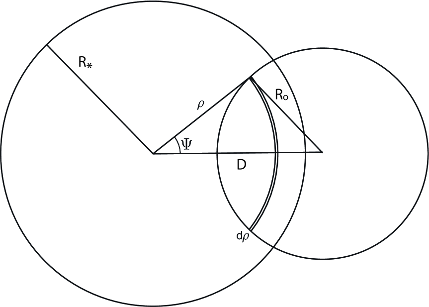
Figure 1: The model of eclipsing binary system. The projection on the picture plane. Here the smaller component is a star or an exoplanet. The geometry of stellar disks in eclipse. Here $\displaystyle{R}_{\scriptscriptstyle{*}}$ is the radius of the eclipsed star, $\displaystyle{R}_{\scriptscriptstyle{o}}$ is the radius of the eclipsing component, $\displaystyle{D}$ is the distance between the centers of the disks of the components, $\rho$, $\Psi$ are respectively the polar radius and the polar angle of a point on the disk of the eclipsed star. The origin is located at the center of the eclipsed star, the polar angle is measured counterclockwise from the radius-vector connecting centers of the star and the transiting component.

Fig. 1 shows the geometry of the stellar disks in eclipse.

The brightness at the point of the disk of the eclipsed star with polar coordinate $\rho$ is given by:

$$J(\rho)=J(0)I\left(\frac{\rho}{\displaystyle{R}_{\scriptscriptstyle{*}}}\right)\,.$$

Here $J(0)$ is the brightness at the center of this stellar disk,

$$I(r)=(1-f(\mu(r))),$$ (1)

$$\mu(r)=\sqrt{1-r^{2}}\,$$

$$f(\mu)=\sum\limits_{k}\Lambda_{k}f_{k}(\mu)\,,$$

where functions $f_{k}$ are such that $f_{k}(1)=0$, are defined by the law of limb-darkening in question, and $\Lambda_{k}$ are the coefficients of limb-darkening.

In this paper we consider the following frequently used limb-darkening laws:

Linear limb-darkening law, for which $f(\mu)=\nobreak\Lambda_{l}f_{l}(\mu)=\nobreak\Lambda_{l}(1-\mu)$;

Square law of limb-darkening, which is characterized by the presence of the term $\Lambda_{q}f_{q}(\mu)=\Lambda_{q}(1-\mu)^{2}$ in the expression for $f$;

Logarithmic limb-darkening law, which is characterized by the presence of the term $\Lambda_{L}f_{L}(\mu)=\nobreak-\Lambda_{L}\mu\ln\mu$ in the expression for $f$;

Square root limb-darkening law, which is characterized by the presence of the term $\Lambda_{Q}f_{Q}(\mu)=\nobreak\Lambda_{Q}(1-\sqrt{\mu})$ in the expression for $f$. , $\sqrt{\mu^{l}}$ , $l$ – .

3 General integral formula for the flux

The decrease of the flux of the binary system due to eclipse is:

$$L^{F}-L(\displaystyle{D},\displaystyle{R}_{\scriptscriptstyle{*}},\displaystyle{R}_{\scriptscriptstyle{o}})=\Delta\!L(\displaystyle{D},\displaystyle{R}_{\scriptscriptstyle{*}},\displaystyle{R}_{\scriptscriptstyle{o}})=\iint\limits_{\displaystyle{S}(\displaystyle{D})}J\left(|\mathbf{R}|\right)d\mathbf{R}\,,$$ (2)

where $L^{F}$ is the unobscured flux of the binary system, $L$ is the obscured flux of the binary system, i.e. the light-curve value, $S(\displaystyle{D})$ is the area of overlapping disks, $\mathbf{R}$ is radius-vector of the point on the stellar disk.

To calculate the integral (2) we introduce the functions:

$$\mathop{\mathcal{A}}\nolimits x\equiv\begin{cases}\pi,&x<-1\\ \arccos x,&-1\leq x\leq 1\\ 0,&x>1\;.\end{cases}$$ (3)

and

$$\mathop{\mathcal{Q}}\nolimits x\equiv\begin{cases}\sqrt{x},&x\geq 0\\ 0,&x<0\;.\end{cases}$$ (4)

Then

$$\frac{d\mathop{\mathcal{A}}\nolimits x}{d\,x}=\-\mathop{\mathcal{Q}}\nolimits\left(\displaystyle{\frac{1}{1-x^{2}}}\right).\\$$ (5)

The relation (5) is obtained naturally by noting that $\mathop{\mathcal{A}}\nolimits z=\mathop{\mathrm{Re}}\arccos z$, $\mathop{\mathcal{Q}}\nolimits x=\mathop{\mathrm{Re}}\sqrt{z}$ for complex number $z$ with $\mathop{\mathrm{Im}}z=0$ and for the functions of complex argument $\arccos$ and $\sqrt{\cdot}$ that are analytic continuations of the inverse cosine and square root of a real argument. Analyticity region is such that $-\pi<\arg z\leq\pi$ for each $z$.

In the polar coordinate system the region of integration $S(\displaystyle{D})$ is given by:

$$S(\displaystyle{D})=\left\{\begin{aligned} &\rho<\displaystyle{R}_{\scriptscriptstyle{*}}\\ &-\pi<\varphi\leq\pi\\ &\frac{\rho^{2}+\displaystyle{D}^{2}-\displaystyle{R}_{\scriptscriptstyle{o}}^{2}}{2\rho\displaystyle{D}}\leq\cos\varphi\,.\end{aligned}\right.$$ (6)

In case of integration (2) with respect to coordinate $\varphi$, for the values of $\rho$, which satisfy $\displaystyle{\left|\frac{\rho^{2}+\displaystyle{D}^{2}-\displaystyle{R}_{\scriptscriptstyle{o}}^{2}}{2\rho\displaystyle{D}}\right|}\leq 1$ variable $\varphi$ takes the values such that

$$\frac{\rho^{2}+\displaystyle{D}^{2}-\displaystyle{R}_{\scriptscriptstyle{o}}^{2}}{2\rho\displaystyle{D}}\leq\cos\varphi\Leftrightarrow|\varphi|\leq\arccos\ \left(\frac{\rho^{2}+\displaystyle{D}^{2}-\displaystyle{R}_{\scriptscriptstyle{o}}^{2}}{2\rho\displaystyle{D}}\right)\,.$$

Hence, the integration over $\varphi$ is from $\displaystyle{-\arccos\ \left(\frac{\rho^{2}+\displaystyle{D}^{2}-\displaystyle{R}_{\scriptscriptstyle{o}}^{2}}{2\rho\displaystyle{D}}\right)}$ to $\displaystyle{\arccos\ \left(\frac{\rho^{2}+\displaystyle{D}^{2}-\displaystyle{R}_{\scriptscriptstyle{o}}^{2}}{2\rho\displaystyle{D}}\right)}$.

For the values of $\rho$, for which $\displaystyle{\frac{\rho^{2}+\displaystyle{D}^{2}-\displaystyle{R}_{\scriptscriptstyle{o}}^{2}}{2\rho\displaystyle{D}}}<-1$ inequality

$$\frac{\rho^{2}+\displaystyle{D}^{2}-\displaystyle{R}_{\scriptscriptstyle{o}}^{2}}{2\rho\displaystyle{D}}<\cos\varphi$$

holds for every value of $\varphi$. In this case, integration with respect to $\varphi$ runs from $-\pi$ to $\pi$.

For the values of $\rho$, for which $\displaystyle{\frac{\rho^{2}+\displaystyle{D}^{2}-\displaystyle{R}_{\scriptscriptstyle{o}}^{2}}{2\rho\displaystyle{D}}}>1$, the last inequality (6) is not satisfied for any values of $\varphi$. Formally, at these values of $\rho$ both integration limits by $\varphi$ are set equal to zero.

Next, using the notation (3) and introducing the function

$$\Psi(\displaystyle{D},x,y)\equiv\mathop{\mathcal{A}}\nolimits\left(\frac{x^{2}+\displaystyle{D}^{2}-y^{2}}{2\,x\,\displaystyle{D}}\right)\,,$$

integral in (2) can be rewritten as:

$$\Delta\!L(\displaystyle{D},\displaystyle{R}_{\scriptscriptstyle{*}},\displaystyle{R}_{\scriptscriptstyle{o}})=\int\limits_{0}^{\displaystyle{R}_{\scriptscriptstyle{*}}}\rho d\rho\int\limits_{-\displaystyle{\Psi(\displaystyle{D},\rho,\displaystyle{R}_{\scriptscriptstyle{o}})}}^{\displaystyle{\Psi(\displaystyle{D},\rho,\displaystyle{R}_{\scriptscriptstyle{o}})}}d\varphi J\left(\rho\right)=\\ =2J(0)\int\limits_{0}^{\displaystyle{R}_{\scriptscriptstyle{*}}}\rho\,\Psi(\displaystyle{D},\rho,\displaystyle{R}_{\scriptscriptstyle{o}})\,I\left(\frac{\rho}{\displaystyle{R}_{\scriptscriptstyle{*}}}\right)d\rho=\\ =J(0)\displaystyle{R}_{\scriptscriptstyle{*}}^{2}\Delta\!L\left(\frac{\displaystyle{D}}{\displaystyle{R}_{\scriptscriptstyle{*}}},1,\frac{\displaystyle{R}_{\scriptscriptstyle{o}}}{\displaystyle{R}_{\scriptscriptstyle{*}}}\right)=J(0)\displaystyle{R}_{\scriptscriptstyle{*}}^{2}\mathbf{\Delta\!L}(\delta,r)\,,$$ (7)

where $r=\frac{\displaystyle{R}_{\scriptscriptstyle{o}}}{\displaystyle{R}_{\scriptscriptstyle{*}}}$, $\delta=\frac{\displaystyle{\displaystyle{D}}}{\displaystyle{R}_{\scriptscriptstyle{*}}}$, and

$$\mathbf{\Delta\!L}(\delta,r)=2\int\limits_{0}^{1}\rho\,\Psi(\delta,\rho,r)\,I(\rho)d\rho=\\ =\int\limits_{0}^{1}\,\Psi(\delta,\sqrt{\rho},r)\,I(\sqrt{\rho})d\rho\,.$$ (8)

Note that $\mathbf{\Delta\!L}(\delta,r)$ is the value of the decrease of the flux of the binary system when radius and brightness at the center of eclipsed star equals unity, radius of the second (eclipsing) component equals $r$ and the distance between centers of disks equals $\delta$. In view of (1) we can express the decrease of the flux as linear combination with limb-darkening coefficients:

$$\mathbf{\Delta\!L}(\delta,r)=\mathbf{\Delta\!L}_{\scriptscriptstyle{0}}(\delta,r)+\Lambda_{l}\mathbf{\Delta\!L}_{l}(\delta,r)+\\ +\Lambda_{q}\mathbf{\Delta\!L}_{q}(\delta,r)+\Lambda_{L}\mathbf{\Delta\!L}_{L}(\delta,r)+\Lambda_{Q}\mathbf{\Delta\!L}_{Q}(\delta,r)\,.$$ (9)

Unobscured flux $L^{f}$ of the star is

$$L^{f}=J(0)R^{2}\pi\mathrm{\mathbf{L}}^{f}$$

when $R$ is the radius of the star, and

$$\mathrm{\mathbf{L}}^{f}=\int\limits_{0}^{1}I(\sqrt{\rho})d\rho=\\ =\mathrm{\mathbf{L}}^{f}_{0}+\Lambda_{l}\mathrm{\mathbf{L}}^{f}_{l}+\Lambda_{q}\mathrm{\mathbf{L}}^{f}_{q}+\Lambda_{L}\mathrm{\mathbf{L}}^{f}_{L}+\Lambda_{Q}\mathrm{\mathbf{L}}^{f}_{Q}\,.$$ (10)

When both components of the binary system are the stars, unobscured flux $L^{F}$ of the binary system is the sum of $L^{f}$ for each star. For binary star and planet $L^{F}$ equals $L^{f}$ for star.

Let $g$ be a function that $g(\rho)$ is a separate linear term in the expression for $I(\sqrt{\rho})$ (given by (1)), $g^{(-1)}\!$ is one of its primitives: $g(\rho)=\displaystyle{\frac{dg^{(-1)}\!(\rho)}{d\rho}}$. We consider the integral of the general form, which is a contribution to $\mathbf{\Delta\!L}(\delta,r)$ caused by the term $g(\rho)$ in the expression for $I(\sqrt{\rho})$:

$$\mathbf{\Delta\!L}_{g}(\delta,r)=\int\limits_{0}^{1}\,\Psi(\delta,\sqrt{\rho},r)\,g(\rho)d\rho\,.$$ (11)

We note that for $\delta>0,r>0$

$$\lim\limits_{\rho\rightarrow 0}\Psi(\delta,\sqrt{\rho},r)=\pi\Theta(r-\delta)\,,$$

where

$$\Theta(t)\equiv\begin{cases}1,&t>0\\ \frac{1}{2},&t=0\\ 0,&t<0\,,\end{cases}\\$$

Using integration by parts, we obtain

$$\mathbf{\Delta\!L}_{g}(\delta,r)=\Psi(\delta,1,r)g^{(-1)}\!(1)-\pi\Theta(r-\delta)g^{(-1)}\!(0)-\\ -\int\limits_{0}^{1}\frac{(\delta^{2}-r^{2}-\rho)g^{(-1)}\!(\rho)}{2\rho}\times\\ \times\mathop{\mathcal{Q}}\nolimits\left(\frac{1}{\left(\rho-\left(\delta-r\right)^{2}\right)\left(\left(\delta+r\right)^{2}-\rho\right)}\right)d\rho\,,$$ (12)

where (5) is used for differentiating $\Psi$.

For non-negative $r$ and $\delta$ the integrand in (12) is non-zero only if $(\delta-r)^{2}<\nobreak\rho<\nobreak(\delta+r)^{2}$. Therefore the integral in (12) is zero if $|\delta-r|\geq\nobreak 1$. And if $|\delta-r|<\nobreak 1$, integrating can be performed over the interval $\left((\delta-r)^{2},\min\left((\delta+r)^{2},1\right)\right)$. In this interval $\arccos\left(\displaystyle{\frac{\delta^{2}+r^{2}-\rho}{2\,\delta\,r}}\right)$ is a monotone function of $\rho$, so we can perform change of variable in integration in the following way:

$$x=\nobreak\arccos\left(\displaystyle{\frac{\delta^{2}+r^{2}-\rho}{2\,\delta\,r}}\right).$$ (13)

Then

$$\rho=\delta^{2}+r^{2}-2r\delta\cos x\,.$$ (14)

Integration with respect to $x$ will be perfomed over the interval

$$\left(0,\arccos\left(\frac{\delta^{2}+r^{2}-\min\left((\delta+r)^{2},1\right)}{2\,\delta\,r}\right)\right)\,.$$

Taking into account the fact that

$$\frac{d}{d\rho}\arccos\left(\frac{\delta^{2}+r^{2}-\rho}{2\,\delta\,r}\right)=\\ =\frac{1}{\sqrt{\left(\rho-\left(\delta-r\right)^{2}\right)\left(\left(\delta+r\right)^{2}-\rho\right)}}\,,$$

and

$$\arccos\left(\frac{\delta^{2}+r^{2}-\min\left((\delta+r)^{2},1\right)}{2\,\delta\,r}\right)=\\ =\mathop{\mathcal{A}}\nolimits\left(\frac{\delta^{2}+r^{2}-1}{2\,\delta\,r}\right)=\Psi(\delta,r,1)\,,$$

we obtain:

$$\mathbf{\Delta\!L}_{g}(\delta,r)=\Psi(\delta,1,r)g^{(-1)}\!(1)-\pi\Theta(r-\delta)g^{(-1)}\!(0)+\\ +\!\!\!\int\limits_{0}^{\displaystyle{\Psi}(\delta,r,1)}\!\!\!\frac{(r^{2}-r\delta\cos x))g^{(-1)}\!(\delta^{2}+r^{2}-2r\delta\cos x)}{\delta^{2}+r^{2}-2r\delta\cos x}dx$$ (15)

Expression (15) is obtained assuming $|\delta-r|<1$. If $|\delta-r|\geq 1$ value of $\Psi(\delta,r,1)=0$ and integral in (15) vanishes. As noted above, when $|\delta-r|\geq 1$, the integral in (12) is zero because the integrand vanishes. Thus, the expression (15) is valid for all positive values of $\delta\text{ and }r$.

By differentiating in (11) integrand with respect to $\delta$ and $r$ we similarly find an expression for the corresponding partial derivative $\mathbf{\Delta\!L}_{g}$:

$$\frac{\partial{\mathbf{\Delta\!L}_{g}(\delta,r)}}{\partial{\delta}}=-2r\!\!\!\!\!\!\!\!\int\limits_{0}^{\displaystyle{\Psi}(\delta,r,1)}\!\!\!\!\!\!\!\!\!\cos x\,g(\delta^{2}+r^{2}-2r\delta\cos x)dx$$ (16)

$$\frac{\partial{\mathbf{\Delta\!L}_{g}(\delta,r)}}{\partial{r}}=2r\!\!\!\!\!\!\!\!\int\limits_{0}^{\displaystyle{\Psi}(\delta,r,1)}\!\!\!\!\!\!\!\!\!g(\delta^{2}+r^{2}-2r\delta\cos x)dx\,.$$ (17)

The contribution to the $\mathrm{\mathbf{L}}^{f}$ caused by the term $g(\rho)$ in the expression for $I(\sqrt{\rho})$:

$$\mathrm{\mathbf{L}}^{f}_{g}=\pi(g^{(-1)}\!(1)-g^{(-1)}\!(0))\,.$$ (18)

4 Individual laws of limb darkening.

The expression for the decrease of the flux due to eclipse of the stellar disk with uniform brightness (with zero coefficients of limb darkening) can be obtained if we put in (15), (16) and (17) $g(x)=1$, $g^{-1}(x)=x$. Then:

$$\mathrm{\mathbf{L}}^{f}_{0}=\pi\,,$$

$$\mathbf{\Delta\!L}_{\scriptscriptstyle{0}}(\delta,r)=\Psi(\delta,1,r)+\Psi(\delta,r,1)r^{2}-\frac{1}{2}Q\left(\delta,r\right)\,,$$ (19)

$$\frac{\partial{\mathbf{\Delta\!L}_{\scriptscriptstyle{0}}(\delta,r)}}{\partial{\delta}}=-\frac{Q(\delta,r)}{\delta}\,,$$ (20)

and

$$\frac{\partial{\mathbf{\Delta\!L}_{\scriptscriptstyle{0}}(\delta,r)}}{\partial{r}}=2\Psi(\delta,r,1)r\,.$$ (21)

Here

$$Q\left(\delta,r\right)\equiv\mathop{\mathcal{Q}}\nolimits\left(\left(1-\left(\delta-r\right)^{2}\right)\left(\left(\delta+r\right)^{2}-1\right)\right)\,.$$

Putting $g(x)=\mu(\sqrt{x})=\sqrt{1-x},\,g^{(-1)}\!(x)=\nobreak-\frac{2}{3}(1-x)^{\frac{3}{2}}$, we get:

$$\mathrm{\mathbf{L}}^{f}_{1}=\frac{2\pi}{3}\,,$$

$$\mathbf{\Delta\!L}_{\scriptscriptstyle{1}}(\delta,r)=\frac{2\pi}{3}\Theta(r-\delta)+\\ +\mathop{\mathcal{Q}}\nolimits\left(\frac{1}{1-(r-\delta)^{2}}\right)\left[\frac{2(\delta+r)}{3(\delta-r)}\hat{\Pi}-\right.\\ -\left.\frac{2}{9}\!\left(3(\delta^{2}-r^{2})+(1-(r-\delta)^{2})((r+\delta)^{2}-1)\right)\!\hat{F}\right]+\\ +\frac{2}{9}\mathop{\mathcal{Q}}\nolimits\left(1-(r-\delta)^{2}\right)(7r^{2}+\delta^{2}-4)\hat{E}\,.\\$$ (22)

Here

$$\hat{\Pi}\equiv\Pi\left(-\frac{4\delta r}{(r-\delta)^{2}};\frac{\Psi(\delta,r,1)}{2}\left|\frac{4\delta r}{1-(r-\delta)^{2}}\right.\right)$$

$$\hat{F}\equiv F\left(\frac{\Psi(\delta,r,1)}{2}\left|\frac{4\delta r}{1-(r-\delta)^{2}}\right.\right)$$

$$\hat{E}\equiv E\left(\frac{\Psi(\delta,r,1)}{2}\left|\frac{4\delta r}{1-(r-\delta)^{2}}\right.\right),$$

where $F,E$ and $\Pi$ are incomplete elliptic integrals of the first, second and third kind:

$$F(\phi\,|m)\equiv\int\limits^{\phi}_{0}\frac{d\theta}{\sqrt{1-m\sin^{2}(\theta)}}\,,$$

$$E(\phi\,|m)\equiv\int\limits^{\phi}_{0}\sqrt{1-m\sin^{2}(\theta)}\,,$$

$$\Pi(n;\phi\,|m)\equiv\int\limits^{\phi}_{0}\frac{d\theta}{(1-n\sin^{2}(\theta))\sqrt{1-m\sin^{2}(\theta)}}\,.$$

The efficient algorithms for their calculations were suggested by Carlson (1994). When $|\delta-r|\rightarrow 0$ or $|\delta-r|\rightarrow 1$, the limit of the term containing the factor $\hat{\Pi}$ in (22) is equal to zero. Note that a similar expression was obtained by Pal (2012) for the integral (primitive) of the appropriately chosen vector field along the limb of the eclipsed component. However, application of this expression for calculation of the flux of the system requires further account of its singularities. Expressions (22) and (19) give direct algorithm for calculating of the brightness, and the possible singularities are taken into account automatically by piecewise smooth functions of one variable $\mathop{\mathcal{A}}\nolimits$ and $\mathop{\mathcal{Q}}\nolimits$

$$\frac{\partial{\mathbf{\Delta\!L}_{\scriptscriptstyle{1}}(\delta,r)}}{\partial{\delta}}=\\ =-2r\!\!\!\!\!\!\!\!\!\int\limits_{0}^{\displaystyle{\Psi}(\delta,r,1)}\!\!\!\!\!\!\!\!\!\,\cos(x)\sqrt{1-(\delta-r)^{2}-4\,\delta r\sin^{2}\left(\frac{x}{2}\right)}\;dx=\\ =-\frac{2}{3\delta}\mathop{\mathcal{Q}}\nolimits\left(1-(r-\delta)^{2}\right)\left[\left((r+\delta)^{2}-1\right)\hat{F}+\right.\\ \left.+\left(1-\delta^{2}-r^{2}\right)\hat{E}\right]\,.$$ (23)

$$\frac{\partial{\mathbf{\Delta\!L}_{\scriptscriptstyle{1}}(\delta,r)}}{\partial{r}}=\\ =2r\!\!\!\!\!\!\!\!\!\int\limits_{0}^{\displaystyle{\Psi}(\delta,r,1)}\!\!\!\!\!\!\!\!\!\,\sqrt{1-(\delta-r)^{2}-4\,\delta r\sin^{2}\left(\frac{x}{2}\right)}\;dx=\\ =4r\mathop{\mathcal{Q}}\nolimits\left(1-(r-\delta)^{2}\right)\hat{E}\,.$$ (24)

For term with linear limb-darkening coefficients in (9):

$$\mathbf{\Delta\!L}_{l}(\delta,r)=\mathbf{\Delta\!L}_{\scriptscriptstyle{1}}(\delta,r)-\mathbf{\Delta\!L}_{\scriptscriptstyle{0}}(\delta,r)\,,$$ (25)

$$\mathrm{\mathbf{L}}^{f}_{l}=\mathrm{\mathbf{L}}^{f}_{1}-\mathrm{\mathbf{L}}^{f}_{0}=-\frac{\pi}{3}\,.$$

Assuming $g(x)=x,\,g^{(-1)}\!(x)=x^{2}/2$ we get:

$\mathrm{\mathbf{L}}^{f}_{2}=\frac{\pi}{2}\,,$

$$\mathbf{\Delta\!L}_{\scriptscriptstyle{2}}(\delta,r)=\frac{1}{2}\Psi(\delta,1,r)+\\ +\frac{r^{2}}{2}\left(2\delta^{2}+r^{2}\right)\Psi(\delta,r,1)-\\ -\frac{1}{8}\left(\delta^{2}+5r^{2}+1\right)Q\left(\delta,r\right)\,.$$ (26)

The partial derivatives $\mathbf{\Delta\!L}_{\scriptscriptstyle{2}}$:

$$\frac{\partial{\mathbf{\Delta\!L}_{\scriptscriptstyle{2}}(\delta,r)}}{\partial{\delta}}=2\delta r^{2}\Psi(\delta,r,1)-\frac{\delta^{2}+r^{2}+1}{2\delta}\,Q(\delta,r)\,,$$ (27)

$$\frac{\partial{\mathbf{\Delta\!L}_{\scriptscriptstyle{2}}(\delta,r)}}{\partial{r}}=2r\left(\delta^{2}+r^{2}\right)\Psi(\delta,r,1)-2rQ(\delta,r)\,,$$ (28)

$$\mathbf{\Delta\!L}_{q}(\delta,r)=\nobreak 2\mathbf{\Delta\!L}_{\scriptscriptstyle{1}}(\delta,r)-\mathbf{\Delta\!L}_{\scriptscriptstyle{0}}(\delta,r)-\mathbf{\Delta\!L}_{\scriptscriptstyle{2}}(\delta,r)\,,$$ (29)

$$\mathrm{\mathbf{L}}^{f}_{q}=2\mathrm{\mathbf{L}}^{f}_{1}-\mathrm{\mathbf{L}}^{f}_{0}-\mathrm{\mathbf{L}}^{f}_{2}=\frac{\pi}{6}\,.$$

Further, we note that

$$\frac{\Psi(\delta,r,1)}{2}=\frac{\pi}{2}-\mathop{\mathcal{A}}\nolimits\mathop{\mathcal{Q}}\nolimits\left(\frac{1-(\delta-r)^{2}}{4\delta r}\right)\,.$$

Assuming $g(x)=\sqrt{1-x}\ln(1-x),\,g^{(-1)}\!(x)=\nobreak{(1-x)}^{3/2}(4/9-2/3\ln(1-x))$ we obtain for the logarithmic limb-darkening law:

$$\mathrm{\mathbf{L}}^{f}_{L}=-\frac{4}{9}\pi\,,$$

$$\mathbf{\Delta\!L}_{L}(\delta,r)=\mathbf{\Delta\!L}_{\scriptscriptstyle{1}}(\delta,r)\left(\ln(4\delta r)-\frac{2}{3}\right)-\\ -\frac{2\pi}{3}\ln(4\delta r)\Theta(r-\delta)-\\ -\frac{8}{3}\sqrt{\delta r}\left[r^{2}\mathop{\mathcal{P}}\nolimits^{L}_{1}\left(\frac{(\delta-r)^{2}}{4\delta r},\frac{1-(\delta-r)^{2}}{4\delta r}\right)-\right.\\ -\left.\delta r\mathop{\mathcal{P}}\nolimits^{L}_{2}\left(\frac{(\delta-r)^{2}}{4\delta r},\frac{1-(\delta-r)^{2}}{4\delta r}\right)\right]$$ (30)

where

$$\mathop{\mathcal{P}}\nolimits^{L}_{1}(n,k)=\\ =\!\!\!\int\limits_{0}^{\displaystyle{\frac{\pi}{2}}-\mathop{\mathcal{A}}\nolimits(\mathop{\mathcal{Q}}\nolimits k)}\!\!\!\!\!\!\frac{\left(k-\sin^{2}x\right)^{\frac{3}{2}}\ln\left(k-\sin^{2}x\right)}{n+\sin^{2}x}\;dx\,,$$ (31)

$$\mathop{\mathcal{P}}\nolimits^{L}_{2}(n,k)=\\ =\!\!\!\int\limits_{0}^{\displaystyle{\frac{\pi}{2}}-\mathop{\mathcal{A}}\nolimits(\mathop{\mathcal{Q}}\nolimits k)}\!\!\!\!\!\!\cos 2x\frac{\left(k-\sin^{2}x\right)^{\frac{3}{2}}\ln\left(k-\sin^{2}x\right)}{n+\sin^{2}x}\;dx$$ (32)

The partial derivatives of $\mathbf{\Delta\!L}_{L}$:

$$\frac{\partial{\mathbf{\Delta\!L}_{L}(\delta,r)}}{\partial{\delta}}=\ln(4\delta r)\frac{\partial{\mathbf{\Delta\!L}_{\scriptscriptstyle{1}}(\delta,r)}}{\partial{\delta}}-\\ -8r\sqrt{r\delta}\mathop{\mathcal{P}}\nolimits^{L}_{\delta}\left(\frac{1-(\delta-r)^{2}}{4\delta r}\right)$$ (33)

$$\mathop{\mathcal{P}}\nolimits^{L}_{\delta}(k)=\\ =\int\limits_{0}^{\displaystyle{\frac{\pi}{2}}-\mathop{\mathcal{A}}\nolimits(\mathop{\mathcal{Q}}\nolimits k)}\!\!\!\!\!\!\!\!\cos 2x\sqrt{k-\sin^{2}x}\ln\left(k-\sin^{2}x\right)\;dx$$ (34)

$$\frac{\partial{\mathbf{\Delta\!L}_{L}(\delta,r)}}{\partial{r}}=\ln(4\delta r)\frac{\partial{\mathbf{\Delta\!L}_{\scriptscriptstyle{1}}(\delta,r)}}{\partial{r}}+\\ +8r\sqrt{r\delta}\mathop{\mathcal{P}}\nolimits^{L}_{r}\left(\frac{1-(\delta-r)^{2}}{4\delta r}\right)$$ (35)

$$\mathop{\mathcal{P}}\nolimits^{L}_{r}(k)=\\ =\int\limits_{0}^{\displaystyle{\frac{\pi}{2}}-\mathop{\mathcal{A}}\nolimits(\mathop{\mathcal{Q}}\nolimits k)}\!\!\!\!\!\!\!\!\sqrt{k-\sin^{2}x}\ln\left(k-\sin^{2}x\right)\;dx$$ (36)

Assuming $g(x)=\sqrt[4]{1-x},\,g^{(-1)}\!(x)=\nobreak-\displaystyle{\frac{4}{5}}(1-x)^{5/4}$, we obtain the following expression for the case of square root limb-darkening law:

$$\mathrm{\mathbf{L}}^{f}_{3}=\frac{4\pi}{5}\,,$$

$$\mathbf{\Delta\!L}_{3}(\delta,r)=\frac{4\pi}{5}\Theta(r-\delta)-\\ -\frac{8}{5}\sqrt[4]{4\delta r}\left[r^{2}\mathop{\mathcal{P}}\nolimits^{Q}_{1}\left(\frac{(\delta-r)^{2}}{4\delta r},\frac{1-(\delta-r)^{2}}{4\delta r}\right)-\right.\\ -\left.\delta r\mathop{\mathcal{P}}\nolimits^{Q}_{2}\left(\frac{(\delta-r)^{2}}{4\delta r},\frac{1-(\delta-r)^{2}}{4\delta r}\right)\right]\,,$$ (37)

where

$$\mathop{\mathcal{P}}\nolimits^{Q}_{1}(n,k)=\!\!\!\int\limits_{0}^{\displaystyle{\frac{\pi}{2}}-\mathop{\mathcal{A}}\nolimits(\mathop{\mathcal{Q}}\nolimits k)}\!\!\!\!\!\!\frac{\left(k-\sin^{2}x\right)^{\frac{5}{4}}}{n+\sin^{2}x}\;dx\,,$$ (38)

$$\mathop{\mathcal{P}}\nolimits^{Q}_{2}(n,k)=\!\!\!\int\limits_{0}^{\displaystyle{\frac{\pi}{2}}-\mathop{\mathcal{A}}\nolimits(\mathop{\mathcal{Q}}\nolimits k)}\!\!\!\!\!\!\cos 2x\frac{\left(k-\sin^{2}x\right)^{\frac{5}{4}}}{n+\sin^{2}x}\;dx\,.$$ (39)

The partial derivatives of $\mathbf{\Delta\!L}_{Q}$:

$$\frac{\partial{\mathbf{\Delta\!L}_{3}(\delta,r)}}{\partial{\delta}}=-4r\sqrt[4]{4r\delta}\mathop{\mathcal{P}}\nolimits^{Q}_{\delta}\left(\frac{1-(\delta-r)^{2}}{4\delta r}\right)$$ (40)

where

$$\mathop{\mathcal{P}}\nolimits^{Q}_{\delta}(k)=\int\limits_{0}^{\displaystyle{\frac{\pi}{2}}-\mathop{\mathcal{A}}\nolimits(\mathop{\mathcal{Q}}\nolimits k)}\!\!\!\!\!\!\!\!\cos 2x\left(k^{2}-\sin^{2}x\right)^{\frac{1}{4}}\!dx$$ (41)

and

$$\frac{\partial{\mathbf{\Delta\!L}_{3}(\delta,r)}}{\partial{r}}=4r\sqrt[4]{4r\delta}\mathop{\mathcal{P}}\nolimits^{Q}_{r}\left(\frac{1-(\delta-r)^{2}}{4\delta r}\right)$$ (42)

where

$$\mathop{\mathcal{P}}\nolimits^{Q}_{r}(k)=\int\limits_{0}^{\displaystyle{\frac{\pi}{2}}-\mathop{\mathcal{A}}\nolimits(\mathop{\mathcal{Q}}\nolimits k)}\!\!\!\!\!\!\!\!\left(k-\sin^{2}x\right)^{\frac{1}{4}}\!dx\,.$$ (43)

For term with square-root limb-darkening coefficients in (9):

$$\mathbf{\Delta\!L}_{Q}(\delta,r)=\mathbf{\Delta\!L}_{3}(\delta,r)-\mathbf{\Delta\!L}_{\scriptscriptstyle{0}}(\delta,r)\,,$$ (44)

$$\mathrm{\mathbf{L}}^{f}_{Q}=\mathrm{\mathbf{L}}^{f}_{3}-\mathrm{\mathbf{L}}^{f}_{0}=-\frac{\pi}{5}\,.$$

The formulas obtained for the square root, it is easy to generalize to the case limb-darkening law contained in the expression for the brightness the term $\sqrt{\mu^{l}}$, where $l$ is an odd positive number, putting in (15), (16) add (17) $g(x)=\sqrt[4]{(1-x)^{l}},\,g^{(-1)}\!(x)=\nobreak-\displaystyle{\frac{4}{4+l}}(1-x)^{1+l/4}$. For an even $l$ of non-multiple 4, light curve and its derivative can be expressed by elliptical integrals similarly to as the formulas (22)–(24) were obtained. If $l$ is divisible by 4 light curve and its derivative can be expressed by elementary functions similarly to as (26)–(28) were obtained for quadratic limb darkening.

5 Numerical calculation of integrals

Thus the calculation of the brightness for the logarithmic and square-root limb-darkening law is reduced to the calculation of integrals $\mathop{\mathcal{P}}\nolimits^{L}_{1}$, $\mathop{\mathcal{P}}\nolimits^{L}_{2}$, $\mathop{\mathcal{P}}\nolimits^{L}_{r}$ $\mathop{\mathcal{P}}\nolimits^{L}_{\delta}$, $\mathop{\mathcal{P}}\nolimits^{L}_{r}$, $\mathop{\mathcal{P}}\nolimits^{L}_{1}$, $\mathop{\mathcal{P}}\nolimits^{Q}_{2}$, $\mathop{\mathcal{P}}\nolimits^{Q}_{r}$ $\mathop{\mathcal{P}}\nolimits^{Q}_{\delta}$, $\mathop{\mathcal{P}}\nolimits^{Q}_{r}$ (depending on parameters). These integrals can be represented in general form:

$$\tilde{\mathop{\mathcal{P}}\nolimits}(n,k)=\!\!\!\int\limits_{0}^{\displaystyle{\frac{\pi}{2}}-\mathop{\mathcal{A}}\nolimits(\mathop{\mathcal{Q}}\nolimits k)}\!\!\!\!\!\!\frac{V(k,x)K\left(k-\sin^{2}x\right)}{n+\sin^{2}x}\;dx\,,$$ (45)

for $\mathop{\mathcal{P}}\nolimits^{L}_{1}$, $\mathop{\mathcal{P}}\nolimits^{L}_{2}$, $\mathop{\mathcal{P}}\nolimits^{Q}_{1}$, $\mathop{\mathcal{P}}\nolimits^{Q}_{2}$ or

$$\bar{\mathop{\mathcal{P}}\nolimits}(k)=\!\!\!\int\limits_{0}^{\displaystyle{\frac{\pi}{2}}-\mathop{\mathcal{A}}\nolimits(\mathop{\mathcal{Q}}\nolimits k)}\!\!\!\!\!\!V(k,x)K\left(k-\sin^{2}x\right)\;dx\,,$$ (46)

for $\mathop{\mathcal{P}}\nolimits^{L}_{r}$ $\mathop{\mathcal{P}}\nolimits^{L}_{\delta}$, $\mathop{\mathcal{P}}\nolimits^{L}_{r}$, $\mathop{\mathcal{P}}\nolimits^{Q}_{r}$ $\mathop{\mathcal{P}}\nolimits^{Q}_{\delta}$, $\mathop{\mathcal{P}}\nolimits^{Q}_{r}$. Here $V(k,x)=\nobreak\sum\limits_{i=1}^{s}u_{i}(k)v_{i}(x)$ where $v_{i}(x)$ are some trigonometric polynomials, $n>0,k>0$. We denote the maximum degree of these trigonometric polynomials as $\tau$. $K(y)=\nobreak\sqrt{y}\ln y$ or $K(y)=\nobreak\sqrt[4]{y^{\gamma}}$, respectively, has a logarithmic or fractional power singularity at $t=0$. In the case of calculating of $\mathop{\mathcal{P}}\nolimits^{Q}_{r}$ $\mathop{\mathcal{P}}\nolimits^{Q}_{\delta}$, $\mathop{\mathcal{P}}\nolimits^{Q}_{r}$, we put $\gamma=1$. For the limb darkening of the general form, which is characterized by the presence of the term $\sqrt{\mu^{l}}$ in the expression for brightness (odd $l$) it is enough to put $\gamma=l\mod 4$.

By applying Gaussian quadrature formula, we can find the numerical value of the integrals with high precision, producing a relatively small number of elementary computations (the amount of computation of the integrand is proportional to required number of significant digits). But at the same time, an integrable function must satisfy certain conditions. In particular, this can be achieved if the higher derivatives of the integrand (or its non-singular component) is uniformly bounded on the section of integration. To reduce the computation of the integrals (45) and (46) to computation of the integrals that satisfy the above conditions, we divide the interval of integration $(0,\displaystyle{\frac{\pi}{2}}-\mathop{\mathcal{A}}\nolimits(\mathop{\mathcal{Q}}\nolimits k))$ sequence $X_{0}>\nobreak X_{1}>\nobreak....>\nobreak X_{M}$, such that $X_{0}=\nobreak\displaystyle{\frac{\pi}{2}}-\mathop{\mathcal{A}}\nolimits(\mathop{\mathcal{Q}}\nolimits k)),\,X_{M}=\nobreak 0$ and

$$\frac{k-\sin^{2}X_{i+1}}{k-\sin^{2}X_{i}}\leq 2\,\,\text{for}\,\,i\geq 1\,\,\text{and}\,\,k\neq 1\,,$$ (47)

$$X_{i}-X_{i+1}\leq\frac{1}{\max\{\tau,2\}}\,\,\text{for all}\,\,i<M\,\,\text{and}\,\,k\,.$$ (48)

In the case of (45) we also require that the following inequality:

$$\frac{n+\cos X_{i}}{n+\cos X_{i+1}}\leq 2\,\,\text{for all}\,\,i<M\,\,\text{and}\,\,k\,.$$ (49)

If $k>1$, inequality from (47) also holds for $i=0$. If $k<1$, then

$$\frac{k-\sin^{2}X_{1}}{(X_{0}-X_{1})\sin(2X_{0})}\leq\frac{3}{2}\,\,\text{and}\,\,X_{1}\geq X_{0}/2\,.$$ (50)

(47)–(50) can be used as recurrent relation, allowing us to construct the sequence ${X_{i}}$.

Thus,

$$\tilde{\mathop{\mathcal{P}}\nolimits}(n,k)=\sum\limits_{i=0}^{M-1}\tilde{\mathop{\mathcal{P}}\nolimits}_{i}(n,k)\,,$$

$$\bar{\mathop{\mathcal{P}}\nolimits}(k)=\sum\limits_{i=0}^{M-1}\bar{\mathop{\mathcal{P}}\nolimits}_{i}(k)\,.$$

where

$$\tilde{\mathop{\mathcal{P}}\nolimits}_{i}(n,k)=\!\!\!\int\limits_{X_{i+1}}^{X_{i}}\frac{V(k,x)K\left(k-\sin^{2}x\right)}{n+\sin^{2}x}\;dx\,,$$ (51)

and

$$\bar{\mathop{\mathcal{P}}\nolimits}_{i}(k)=\!\!\!\int\limits_{X_{i+1}}^{X_{i}}V(k,x)K\left(k-\sin^{2}x\right)\;dx\,,$$ (52)

For fixed values of $n$ and $k$ the two last integrals can be represented in general form:

$$\mathop{\mathcal{P}}\nolimits_{i}=\!\!\!\int\limits_{X_{i+1}}^{X_{i}}U(x)K\left(k-\sin^{2}x\right)\;dx\,,$$

where $U(x)=\nobreak\displaystyle{\frac{V(k,x)}{n+\sin^{2}x}}$ for (51) and $U(x)=\nobreak V(k,x)$ for (52).

By linear substitution of variable of integration

$$x(t)=X_{i+1}+t(X_{i}-X_{i+1})$$

in (53), we turn to the integration from zero to unity:

$$\mathop{\mathcal{P}}\nolimits_{i}=(X_{i}-X_{i+1})\int\limits_{0}^{1}U(x(t))K\left(k-\sin^{2}(x(t))\right)\;dt\,.$$ (53)

In this form, $\mathop{\mathcal{P}}\nolimits_{i}$ can be computed by applying the Gaussian quadrature formula:

$$\int\limits_{0}^{1}h(t)\omega(t)dt\approx\sum\limits_{l=1}^{N}w_{l}h(t_{l})\,.$$ (54)

Here $\omega(t)>0\,\forall t\in(0,1)$, nodes $t_{i}$ are the roots of the polinomial $H_{N}(t)$, where $\{H_{i}\}$ is the system of orhtogonal polynomials with weight $\omega$ in the interval $(0,1)$:

$$\int\limits_{0}^{1}H_{l}(t)H_{j}(t)\omega(t)dt=0\,\text{for }l\neq j\,.$$

$w_{l}$ can be found as the solution of the system of $N$ linear algebraic equations, which can be obtained if we put $h(t)\equiv\nobreak 1,h(t)\equiv\nobreak t,\ldots,h(t)\equiv\nobreak t^{N}$ in (54) and replace the approximate equality with exact equality.

$N$ can be adjusted so as to ensure the required accuracy of calculation of $\mathop{\mathcal{P}}\nolimits_{0i}(n,k),\mathop{\mathcal{P}}\nolimits_{di}(k)$ and can be the same for all values of $i,n,k$. $N$ is of the same order of magnitude as the number of significant digits in the result, and this allows to calculate the integral with the required accuracy in a reasonable time. So, after calculation of the roots of polynomials $x_{l}$ and weights $w_{l}$ (this may take a while), we can re-use them for computing $\mathop{\mathcal{P}}\nolimits_{0i}(n,k),\mathop{\mathcal{P}}\nolimits_{di}(k)$ for all $i,n,k$.

In the case of $i>0$ or of $k>1$ we put in (54): $\omega(t)=1\forall t\in(0,1)$, $h(t)=\nobreak{(X_{i}-X_{i+1})U(x(t))K\left(k-\sin^{2}x(t)\right)}$. Then

$$\mathop{\mathcal{P}}\nolimits_{i}\approx\sum\limits_{l=1}^{N}w_{l}h(t_{l})\,.$$

Note that in this case $H_{i}(t)\equiv P_{i}(2t-1)$ where $P_{i}$ are Legendre polynomials.

In the case of $i>0$, $k<1$ and logarithmic limb-darkening law ($K(y)=\nobreak\sqrt{y}\ln y$) we represent the integrand from (53) in the form:

$$U(x(t))\sqrt{1-t}\sqrt{\frac{k-\sin^{2}(x(t))}{1-t}}\times\\ \times\left[\ln\left(\frac{k-\sin^{2}(x(t))}{1-t}\right)+\ln(1-t)\right]$$

Next, we put in (54): $\omega(t)=\sqrt{1-t}\forall t\in(0,1)$,

$$h(t)=U(x(t))\sqrt{\frac{k-\sin^{2}(x(t))}{1-t}}\ln\left(\frac{k-\sin^{2}(x(t))}{1-t}\right).$$

Note that here $H_{i}(t)\equiv P^{(\frac{1}{2},0)}_{i}(2t-1)$ where $P^{(\frac{1}{2},0)}_{i}$ are Jacobi polynomials. Let $S_{1}=\nobreak\sum\limits_{l=1}^{N}w_{l}h(t_{l})$.

Next, we put in (54): $\omega(t)=\nobreak{-\sqrt{1-t}\ln(1-t)\forall t\in(0,1)}$,

$$h(t)=-U(x(t))\sqrt{\frac{k-\sin^{2}(x(t))}{1-t}}.$$

The polynomials corresponding to this value of $\omega$ can be obtained through the standard procedure of orthogonalization. Let $S_{2}=\nobreak\sum\limits_{l=1}^{N}w_{l}h(t_{l})$. Then $\mathop{\mathcal{P}}\nolimits_{0}\approx{(S_{1}+S_{2})(X_{0}-X_{1})}$.

In the case of $i>0$, $k=1$ and logarithmic limb-darkening law ($K(y)=\nobreak\sqrt{y}\ln y$) we represent the integrand from (53) in the form:

$$2U(x(t))\cos(x(t))\left[\ln\left(\frac{\cos(x(t))}{1-t}\right)+\ln(1-t)\right]$$

Next, we put in (54): $\omega(t)=\nobreak 1\forall t\in(0,1)$,

$$h(t)=2U(x(t))\cos(x(t))\ln\left(\frac{\cos(x(t))}{1-t}\right).$$

Let $S_{1}=\nobreak\sum\limits_{l=1}^{N}w_{l}h(t_{l})$.

Next, we put in (54): $\omega(t)=\nobreak{-\ln(1-t)\forall t\in(0,1)}$,

$$h(t)=-2U(x(t))\cos(x(t).$$

Let ${S_{2}=\sum\limits_{l=1}^{N}w_{l}h(t_{l})}$. Then $\mathop{\mathcal{P}}\nolimits_{0}\approx\nobreak{(S_{1}+S_{2})(X_{0}-X_{1})}$.

In the case of $i>0$, $k<1$ and square-root limb-darkening law ($K(y)=\nobreak\sqrt[4]{y^{\gamma}}$), we put in (54): $\omega(t)=\nobreak(1-t)^{\frac{\gamma}{4}}\forall t\in(0,1)$,

$$h(t)=U(x(t))\left(\frac{k-\sin^{2}x(t)}{1-t}\right)^{\frac{\gamma}{4}}.$$

Note that here $H_{i}(t)\equiv\nobreak P^{(\frac{\gamma}{4},0)}_{i}(2t-1)$ where $P^{(\frac{\gamma}{4},0)}_{i}$ are Jacobi polynomials. Then $\mathop{\mathcal{P}}\nolimits_{0}\approx\nobreak{(X_{0}-X_{1})\sum\limits_{l=1}^{N}w_{l}h(t_{l})}$.

In the case of $i>0$, $k=1$ and square-root limb-darkening law, we put in (54): $\omega(t)=\sqrt{1-t}\,\forall t\in\nobreak(0,1)$,

$$h(t)=U(x(t))\left(\frac{\cos(x(t))}{1-t}\right)^{\frac{\gamma}{2}}.$$

Then $\mathop{\mathcal{P}}\nolimits_{0}\approx\nobreak{(X_{0}-X_{1})\sum\limits_{l=1}^{N}w_{l}h(t_{l})}$.

Calculations show that in all cases of the applications of the Gauss quadrature accuracy of 19 significant decimal digits (corresponding to 80-bit machine numbers) can be achieved by choosing the $N$ to be 14. Value sets of points $t_{i}$ and weights $w_{i}$ corresponding to each of the considered forms of the function $\omega$, can be downloaded from the Internet, along with other materials (see Conclusion).

6 Conclusion

We have derived the expression for the calculation of the eclipsing binary flux and its derivatives. We considered the linear limb-darkening law, the quadratic limb-darkening law, the logarithmic limb-darkening law, and the square root limb-darkening law. In general, the decrease of the flux is given by the expression (9). In (19)-(21), $\mathbf{\Delta\!L}_{0}$ corresponds to uniform brightness and its derivatives, it is expressed in terms of easily computed piecewise-defined functions of one variable $\mathop{\mathcal{A}}\nolimits\,\,$(3) and $\mathop{\mathcal{Q}}\nolimits\,\,$ (4). $\mathbf{\Delta\!L}_{l}$ corresponds to the linear limb-darkening law, given as linear combination of $\mathbf{\Delta\!L}_{0}$ and $\mathbf{\Delta\!L}_{1}$ (44), where $\mathbf{\Delta\!L}_{1}$ with its derivatives is expressed in terms of incomplete elliptic integrals in (22)-(24). $\mathbf{\Delta\!L}_{q}$ corresponds to the quadratic limb-darkening law, given as linear combination of $\mathbf{\Delta\!L}_{0}$, $\mathbf{\Delta\!L}_{1}$ and $\mathbf{\Delta\!L}_{1}$ (29), where $\mathbf{\Delta\!L}_{2}$ with its derivatives is given in (26)-(28). $\mathbf{\Delta\!L}_{L}$ corresponds to the logarithmic limb-darkening and $\mathbf{\Delta\!L}_{Q}$ corresponds to the square-root limb-darkening expressed by two- and one-parametric integrals. Further, we described how these integrals can be found numerically by multiple application of the Gaussian quadrature formula. It is important that the nodes for this formula can be found once and re-used for the calculations for different values of parameters. Also, the general integral form (15)–(17) of the flux component allows us to extend this approach to other limb-darkening laws.

The algorithm described above was tested by Abubekerov et al. (2010, 2011); Gostev (2011) for the interpretation of the high-precision polychrome light-curves of the binary system with exoplanets HD 209458 Brown et al. (2001) , HD 189733 Pont et al. (2007) and monochrome light-curves of Kepler-5b, Kepler-6b, Kepler-7b Koch et al. (2010); Dunham et al. (2010); Latham et al. (2010).

The algorithm is implemented in ANSI C in the form of the functions for computation of the individual component $\mathbf{\Delta\!L}(\delta,r)$ and its derivatives. This implementation is available from http://lnfm1.sai.msu.su/$\sim$ngostev/algorithm.html

This work was supported by the President of Russian Federation grant MK-893.2012.2, RFBR grant 12-02-31466.