Density-functional theory for the spin-1 bosons in a one-dimensional harmonic trap

Abstract

We propose the density-functional theory for one-dimensional harmonically trapped spin-1 bosons in the ground state with repulsive density-density interaction and anti-ferromagnetic spin-exchange interaction. The density distributions of spin singlet paired bosons and polarized bosons with different total polarization for various interaction parameters are obtained by solving the Kohn-Sham equations which are derived based on the local density approximation and the Bethe ansatz exact results for homogeneous system. Non-monotonicity of the central densities is attributed to the competition between the density interaction and spin-exchange. The results reveal the phase separation of the paired and polarized bosons, the density profiles of which respectively approach the Tonks-Girardeau gases of Bose-Bose pairs and scalar bosons in the case of strong interaction. We give the R-P phase diagram at strong interaction and find the critical polarization, which paves the way to direct observe the exotic singlet pairing in spinor gas experimentally.

I Introduction

Spinor Bose gases and one-dimensional (1D) system are both the fascinating topics in the research of cold atoms Kawaguchi2012 ; Kurn2012 ; Cazalilla2011 ; GuanRMP . The studies of their crossing point for 1D spinor bosons are also attractive in theories Wenxian2005PRA71 ; yajiang2006 ; Cao2007 ; Deuretzbacher2008 ; Girardeau2011 ; Essler2009 ; Lee2009 ; Kuhn2012 and have been realized in recent experiments Liao2010 ; Campbell2012 ; Vinit2012 . Spinor gases are prepared in the optical traps where the induced electric dipole moment determines the laser-atom interaction and involve an ensemble of Bose atoms condensed in a coherent superposition of all possible hyperfine states. The early experimentally achieved spinor gases include ²³Na Kurn1998 ; Miesner1999 and ⁸⁷Rb Matthews1999 ; Barrett2001 . In the three-dimensional (3D) case, the spin-dependent spin-exchange interactions are much weaker than the spin-independent short-range density-density interactions, for example, the ratio of them are $c_{2}/c_{0}\left(\text{Na}\right)=0.03$ Crubellier1999 and $c_{2}/c_{0}\left(\text{Rb}\right)=-0.005$ Kempen2002 respectively. The ground-state wavefunction is represented by a spinor wavefunction which minimizes the free energy Ohmi1998 ; Tianlun1998 ; Koashi2000 and the spin-exchange interactions give rise to a rich variety of phenomena such as spin domains Miesner1999 , textures Ohmi1998 , spin mixing dynamics Law1998 ; Pu1999 ; Wenxian2005PRA72 ; zhangjie2011 , and fragmentation of condensate Tianlun2000 ; Mueller2006 ; zhangjie2010 etc. On the other hand, 1D systems can be realized by confining the cold atoms in strong anisotropic traps where the motion of atoms is effectively 1D Greiner2001 ; Moritz2003 ; Paredes2004 ; Kinoshita2004 ; Haller2009 ; Liao2010 ; Campbell2012 ; Vinit2012 . The interaction among the atoms can be tuned in the whole regime of interaction strength via the idea of Feshbach resonance as well as the confinement-induced resonance (CIR) Olshanii1998 ; Bergeman ; Sinha . These experimental developments have provided unprecedented opportunities for testing the theory of 1D exactly solvable many-body models Lieb1963 ; Yang1967 ; Yang1968 ; Fuchs2004 ; Imambekov2006 ; Imambekov2003 ; Sutherland1968 ; Cao2007 .

Many theories have studied the 1D spinor gases. Under the mean-field theory, Zhang and You checked the validity of a Gaussian ansatz for the transverse profile in the weak interaction regime and a Thomas-Fermi ansatz (TFA) in the strong interaction regime Wenxian2005PRA71 . Hao et al. yajiang2006 modified the Gross-Pitaevskii (GP) equations based on the solution of Lieb-Lininger (L-L) Lieb1963 model to reveal that the total densities of the 1D spinor bosons exhibit the Tonks-Girardeau (TG) Girardeau1960 properties of 1D scalar bosons when density-density interaction is strong enough. The detailed TG and super Tonks-Girardeau gas (STG) properties of 1D spinor bosons have been investigated particularly by Deuretzbacher et al. Deuretzbacher2008 and Girardeau et al. Girardeau2011 with the method of Bose-Fermi mapping.

If the spin-exchange interaction can be modulated to the order of density-density interaction, the competition between these two kinds of interaction must be considered. Cao et al. find that the 1D homogeneous spinor bosons under $c_{0}=c_{2}$ can be exactly solved with Bethe ansatz (BA) method Cao2007 . Essler et al. show its low-energy degrees of freedom are equivalent to a spin-charge separation theory of the U(1) Tomonaga-Luttinger liquid describing the charge sector and the O(3) nonlinear $\sigma$ model describing the spin sector Essler2009 . By means of the thermodynamical Bethe ansatz (TBA) method Lee2009 ; Kuhn2012 , Lee et al. and Kuhn et al. give the ground state phase diagram and investigate the universal thermodynamics and quantum criticality of the trapped 1D spinor bosons for the strong interaction situation.

So far, a method is not available for the 1D trapped spin-1 bosons in the entire region of interaction from weak to strong. In this paper, we develop the Hohenberg-Kohn-Sham density functional theory (DFT) to investigate the ground-state properties of 1D harmonically trapped spin-1 bosons. DFT has been widely used for treating electron systems with long-range Coulomb interaction HohenbergKohn ; Dreizler1990 . It also has been successfully generalized to cold atom systems with short-range contact interaction Nunes ; Kim ; Albus ; Ma2012 . For 1D cold-atom systems, the method of DFT based on BA results has been developed to solve the ground state problem of bosons Kim ; Brand ; Yajiang2009 , fermions Astrakharchik ; Xianlong and Bose-Fermi mixtures Hongmei2012 .

Here we apply this method to study how the ground state of 1D trapped spin-1 bosons evolves along with the interaction strength from weak to strong. We derive the Kohn-Sham (KS) equations by combing the BA solutions and Local Density Approximation (LDA). The ground state densities and energies for different interactions are obtained by solving these equations iteratively. The paper is organized as follows. We introduce our theory in Sec. II and show the numerical results in Sec. III. The theory part includes the model, the BA equation for homogeneous system and the KS equations for trapped system. In the results part, we first show the case that all bosons are fully paired and then for the partially paired case.

II Theory

II.1 Model

We consider $N$ spin-1 bosons of mass $m$ confined in extremely anisotropic crossed optical dipole traps with delta-function type density-density interaction and spin exchange interaction between atoms. The trap is characterized by the radial and axial angular frequencies $\omega_{\bot}$ and $\omega$ with corresponding harmonic oscillator lengths $a_{\bot}=\sqrt{\hbar/m\omega_{\bot}}$ and $a=\sqrt{\hbar/m\omega}$ respectively. When $\omega_{\bot}$ $\gg$ $\omega$, the radial Thomas-Fermi radius is small enough such that only axial spin domains could form Campbell2012 ; Vinit2012 . In first quantized form, the Hamiltonian for 1D spin-1 gas can be written as

$$H = \sum_{i=1}^{N}\left(-\frac{\hbar^{2}}{2m}\frac{\partial^{2}}{\partial x_{i}^{2}}+\frac{1}{2}m\omega^{2}x_{i}^{2}\right)$$ (1)

$$+\sum_{i<j}\left[c_{0}^{1D}+c_{2}^{1D}\mathbf{S}_{i}\cdot\mathbf{S}_{j}\right]\delta\left(x_{i}-x_{j}\right),$$

where $\mathbf{S}_{i,j}$ are spin-1 operators, $c_{0}^{1D}$ and $c_{2}^{1D}$ are 1D interaction parameters which can be expressed through interaction parameters $g_{S}^{1D}$ in total spin $S=0,2$ channels as $c_{0}^{1D}=\left(g_{0}^{1D}+2g_{2}^{1D}\right)/3$ and $c_{2}^{1D}=\left(g_{2}^{1D}-g_{0}^{1D}\right)/3$. In experiments, $g_{S}^{1D}$ can be tuned with $a_{\bot}$ and 3D s-wave scattering length $a_{S}^{3D}$ according to $g_{S}^{1D}=2\hbar^{2}a_{S}^{3D}/ma_{\bot}^{2}\left(1-Aa_{S}^{3D}/a_{\bot}\right)$ with constant $A=1.0326$ Olshanii1998 . Thus $c_{0}^{1D}$ and $c_{2}^{1D}$ may be manipulated in wider range comparing with 3D spinor system.

The number of atoms $N_{+}$, $N_{0}$ and $N_{-}$ corresponding to spin states $s=+1,0,-1$ are not conserved because the scattering between two atoms of spin $s=\pm 1$ can produce two atoms of spin $s=0$ and vice versa, whereas the total number of atoms $N=N_{+}+N_{0}+N_{-}$ and total spin in the $z$ component $S^{z}=N_{+}-N_{-}$ are conserved yet. Therefore we may consider the system is composed of two parts of atoms, particle I and particle II with total particle numbers $N=N_{1}+2N_{2}$ and total polarization $P=N_{1}/N$. The number of particle I is $N_{1}=S^{z}$ where all atoms have parallel spin forming the ferromagnetic phase. The number of particle II is $2N_{2}$ where $N_{2}$ pairs of atoms are formed between two spin states $s=\pm 1$ or between two spin states $s=0$. Here we have supposed that $N_{+}\geqslant N_{-}$ and that $N_{0}$ is even. The sign of $c_{0}^{1D}$ determines that the interactions between the bosons are repulsive or attractive, while the sign of $c_{2}^{1D}$ determines that the spin exchange interaction in the pairs are ferromagnetic or anti-ferromagnetic.

II.2 Bethe ansatz equations for homogeneous system

With the particles confined in a finite 1D tube with length $L$ instead of a harmonic trap as in the Hamiltonian (1), the system has been exactly solved by Cao et al. Cao2007 with BA method under a special condition

$$c_{0}^{1D}=c_{2}^{1D}=g>0,$$

i.e., the repulsive density-density interaction equals the antiferromagnetic spin-exchange interaction. They gave the BA equations

$$e^{ik_{j}L}=\prod\limits_{i=1,i\neq j}^{N}\tilde{e}_{4}\left(k_{j}-k_{i}\right)\prod\limits_{\alpha=1}^{2N_{2}}\tilde{e}_{-2}\left(k_{j}-\Lambda_{\alpha}\right),$$ (2)

$$\prod\limits_{i=1}^{N}\tilde{e}_{2}\left(\Lambda_{\alpha}-k_{i}\right)=-\prod\limits_{\beta=1}^{2N_{2}}\tilde{e}_{2}\left(\Lambda_{\alpha}-\Lambda_{\beta}\right),$$ (3)

with $\tilde{e}_{n}\left(x\right)=\left(x+inc^{\prime}\right)/\left(x-inc^{\prime}\right)$, $c^{\prime}=c/4$ and $c=2mg/\hbar^{2}$. $\left\{k_{i}\right\}$ in the equations is the set of quasi-momentum and $\left\{\Lambda_{\alpha}\right\}$ is the set of the spin rapidity. The ground state energy of the system is

$$E=\frac{\hbar^{2}}{2m}\sum_{i=1}^{N}k_{i}^{2}.$$ (4)

For positive $c_{2}^{1D}$, the spin-exchange interaction is antiferromagnetic. $2N_{2}$ particles form spin singlet bound pairs between two spin $s=\pm 1$ atoms or between two spin $s=0$ atoms, whereas $N_{1}$ particles are polarized. The equations (2) and (3) have $N_{1}$ real solutions for $k_{i}$ ($i=1,\cdots N_{1}$) and $N_{2}$ pairs conjugate complex solutions or string solutions for $k_{\alpha}$ and $\Lambda_{\alpha}$ ($\alpha=1,\cdots,2N_{2}$), i.e.

$$k_{\alpha} = \lambda_{l}\pm ic^{\prime},$$

$$\Lambda_{\alpha} = \lambda_{l}\pm ic^{\prime},$$ (5)

with $\lambda_{l}$ ($l=1,\cdots,N_{2}$) real numbers Cao2007 ; Lee2009 . Inserting (5) into (2) (3) and adopting the thermodynamic limit, i.e., the length of gas $L\rightarrow\infty$ and particle numbers $N,N_{1},N_{2}\rightarrow\infty$ with densities $n=N/L$, $n_{1}=N_{1}/L$ and $n_{2}=N_{2}/L$ finite, we easily arrive at the BA integral equations

$$2\pi\rho_{1}\left(k\right) = 1+2\int_{-B}^{B}dk^{\prime}\rho_{1}\left(k^{\prime}\right)a_{4}\left(k,k^{\prime}\right)$$ (6)

$$+2\int_{-Q}^{Q}d\lambda\rho_{2}\left(\lambda\right)\left(a_{5}-a_{1}\right)\left(k,\lambda\right),$$

$$\pi\rho_{2}\left(\lambda\right) = 1+\int_{-B}^{B}dk\rho_{1}\left(k\right)\left(a_{5}-a_{1}\right)\left(k,\lambda\right)$$ (7)

$$+\int_{-Q}^{Q}d\lambda^{\prime}\rho_{2}\left(\lambda^{\prime}\right)\left(a_{6}+a_{4}-a_{2}\right)\left(\lambda,\lambda^{\prime}\right),$$

where

$$\left(a_{n}-a_{m}\right)\left(x_{1},x_{2}\right)=a_{n}\left(x_{1},x_{2}\right)-a_{m}\left(x_{1},x_{2}\right),$$ (8)

and

$$a_{n}\left(x_{1},x_{2}\right)=\frac{n\left|c^{\prime}\right|}{\left(nc^{\prime}\right)^{2}+\left(x_{1}-x_{2}\right)^{2}},$$ (9)

with $\rho_{1}\left(k\right)$ and $\rho_{2}\left(\lambda\right)$ densities of $k$ and $\lambda$. The integral boundaries $B$ and $Q$ are determined by the conditions

$$n_{1} = \int_{-B}^{B}dk\rho_{1}\left(k\right),$$ (10)

$$n_{2} = \int_{-Q}^{Q}d\lambda\rho_{2}\left(\lambda\right).$$ (11)

From (4), we get the ground state energy per unit length

$$\frac{E}{L} = \frac{\hbar^{2}}{2m}\int_{-B}^{B}dkk^{2}\rho_{1}\left(k\right)$$ (12)

$$+\frac{\hbar^{2}}{2m}\int_{-Q}^{Q}d\lambda 2\lambda^{2}\rho_{2}\left(\lambda\right)-\epsilon_{b}n_{2},$$

where the binding energy of the pair in defined as

$$\epsilon_{b}=\frac{\hbar^{2}}{2m}\frac{c^{2}}{8}.$$ (13)

To solve the BA equations, we introduce the dimensionless L-L interaction parameter $\gamma=c/2n=mg/\hbar^{2}n$ and polarization parameter $p=n_{1}/n$. Let $k=Bx$, $\lambda=Qy$, $B=c/\beta_{1}$ and $Q=c/\beta_{2}$, the densities of quasi-momentum and spin rapidity turn out to be $\rho_{1}\left(k\right)=g_{1}\left(x\right)$ and $\rho_{2}\left(\lambda\right)=g_{2}\left(y\right)$. The integral BA equations (6) and (7) are translated into

$$2\pi g_{1}\left(x\right) = 1+\frac{2}{\beta_{1}}\int_{-1}^{1}dx^{\prime}g_{1}\left(x^{\prime}\right)b_{4}\left(\frac{x}{\beta_{1}},\frac{x^{\prime}}{\beta_{1}}\right)$$

$$+\frac{2}{\beta_{2}}\int_{-1}^{1}dyg_{2}\left(y\right)\left(b_{5}-b_{1}\right)\left(\frac{x}{\beta_{1}},\frac{y}{\beta_{2}}\right),$$

$$\pi g_{2}\left(y\right) = 1+\frac{1}{\beta_{1}}\int_{-1}^{1}dxg_{1}\left(x\right)\left(b_{5}-b_{1}\right)\left(\frac{x}{\beta_{1}},\frac{y}{\beta_{2}}\right)$$

$$+\frac{1}{\beta_{2}}\int_{-1}^{1}dy^{\prime}g_{2}\left(y^{\prime}\right)\left(b_{6}+b_{4}-b_{2}\right)\left(\frac{y}{\beta_{2}},\frac{y^{\prime}}{\beta_{2}}\right),$$

with

$$\left(b_{n}-b_{m}\right)\left(x_{1},x_{2}\right)=b_{n}\left(x_{1},x_{2}\right)-b_{m}\left(x_{1},x_{2}\right),$$ (16)

and

$$b_{n}\left(x_{1},x_{2}\right)=\frac{n/4}{\left(n/4\right)^{2}+\left(x_{1}-x_{2}\right)^{2}}.$$ (17)

The normalization conditions (10) and (11) are now

$$\beta_{1} = \frac{2\gamma}{p}\int_{-1}^{1}g_{1}\left(x\right)dx,$$ (18)

$$\beta_{2} = \frac{4\gamma}{1-p}\int_{-1}^{1}g_{2}\left(y\right)dy.$$ (19)

From (12) the ground state energy per atom for the homogeneous 1D spinor gas is

$$\varepsilon^{\hom}\left(n,\gamma,p\right)=\frac{E}{N}=\frac{\hbar^{2}n^{2}}{2m}e\left(\gamma,p\right),$$ (20)

with

$$e\left(\gamma,p\right)=e_{1}\left(\gamma,p\right)+e_{2}\left(\gamma,p\right)+e_{b}\left(\gamma,p\right)$$ (21)

and

$$e_{1}\left(\gamma,p\right) = \frac{8\gamma^{3}}{\beta_{1}^{3}}\int_{-1}^{1}x^{2}g_{1}\left(x\right)dx,$$ (22)

$$e_{2}\left(\gamma,p\right) = \frac{16\gamma^{3}}{\beta_{2}^{3}}\int_{-1}^{1}y^{2}g_{2}\left(y\right)dy,$$ (23)

$$e_{b}\left(\gamma,p\right) = -\frac{\gamma^{2}\left(1-p\right)}{4}.$$ (24)

Here (22) and (23) can be solved numerically with the combination of integral equations (II.2), (II.2) and the normalization (18), (19). The chemical potentials are taken as the derivatives of (20) as

$$\mu_{1}^{\hom}\left(n,\gamma,p\right) = \frac{\partial(n\varepsilon^{\hom})}{\partial n_{1}}=\frac{\hbar^{2}n^{2}}{2m}f_{1}\left(\gamma,p\right),$$ (25)

$$\mu_{2}^{\hom}\left(n,\gamma,p\right) = \frac{\partial(n\varepsilon^{\hom})}{\partial n_{2}}=\frac{\hbar^{2}n^{2}}{2m}f_{2}\left(\gamma,p\right),$$ (26)

where

$$f_{1}\left(\gamma,p\right) = 3e-\gamma\frac{\partial e}{\partial\gamma}+\left(1-p\right)\frac{\partial e}{\partial p},$$ (27)

$$f_{2}\left(\gamma,p\right) = 2\left(3e-\gamma\frac{\partial e}{\partial\gamma}-p\frac{\partial e}{\partial p}\right).$$ (28)

We see that, when $p=1$, the system is in a pure ferromagnetic phase with spin-polarized bosons. Here $e\left(\gamma,p=1\right)$ coincides with $e\left(\gamma\right)$ in the L-L model of scalar bosons Lieb1963 with interaction parameter $2\gamma$. When $p=0$, all the bosons form pairs and the system is in a pure antiferromagnetic phase. In the limiting case of $\gamma=0$, the system reduces to free bosons with $e\left(\gamma=0,p\right)=0$. When $\gamma$ is very strong, the integral equations (II.2) and (II.2) give $g_{1}\left(x\right)\approx 1/2\pi$ and $g_{2}\left(x\right)\approx 1/\pi$, then

$$e\left(\gamma\rightarrow+\infty,p\right)\approx\frac{\pi^{2}p^{3}}{3}+\frac{\pi^{2}\left(1-p\right)^{3}}{48}-\frac{\gamma^{2}\left(1-p\right)}{4}.$$ (29)

The energy per unit length in the strong interaction case

$$\frac{E}{L}\approx\frac{\hbar^{2}}{2m}\left(\frac{\pi^{2}n_{1}^{3}}{3}+\frac{\pi^{2}n_{2}^{3}}{6}-\frac{c^{2}n_{2}}{8}\right),$$ (30)

is composed of three parts: the energy density of $N_{1}$ free fermions with mass $m$ in Ref. Hongmei2012 , the energy density of $N_{2}$ free composite fermions with mass $2m$, and the binding energy $N_{2}\epsilon_{b}/L$ of the composite fermions. This shows that stronger interactions favors the forming of boson-boson pairs. The chemical potentials in this case are

$$\mu_{1}^{\hom}\left(\gamma\rightarrow+\infty,p\right) \approx \frac{\hbar^{2}}{2m}\pi^{2}n_{1}^{2},$$ (31)

$$\mu_{2}^{\hom}\left(\gamma\rightarrow+\infty,p\right) \approx \frac{\hbar^{2}}{2m}\left(\frac{\pi^{2}}{2}n_{2}^{2}-\frac{c^{2}}{8}\right).$$ (32)

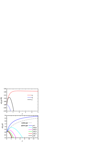
Figure 1: (Color Online) The function $e\left(\gamma,p\right)$ for the ground state energy of 1D homogeneous spin-1 bosons. In the upper panel, $p=0$. In the lower panel the real lines are for $p=0,0.2,0.4,0.6,0.8,1$ from bottom to top and the dash-dotted line is for scalar bosons.

In Fig. 1, we plot the interaction dependence of energy density $e\left(\gamma,p\right)$ for various polarization $p$ and compare it with the case of scalar bosons. The upper figure is for $p=0$, i.e., all the bosons form the pairs. Clearly we have $e_{1}=0$ and $e_{2}\left(\gamma\right)$ (red dashed line), which is obtained numerically from the combination of (II.2), (19) and (23), increases linearly along with $\gamma$ for $\gamma\ll 1$ and approaches slowly to a constant value $\pi^{2}/48$ for $\gamma\gg 1$. $e_{2}\left(\gamma\right)$ and the inverse parabola function $e_{b}\left(\gamma\right)=-\gamma^{2}/4$ together dictate that $e\left(\gamma\right)$ is not monotonic and has a maximum value $0.1169$ at $\gamma=0.4$. The lower figure is for $e\left(\gamma,p\right)$ with $p=0,0.2,0.4,0.6,0.8,1$ corresponding to the real lines from bottom to top. It shows that the energy function $e\left(\gamma,p\right)$ increases along with $p$ for the same parameter $\gamma$. For $p=1$, i.e., pure ferromagnetic phase case, $e\left(\gamma\right)$ increases monotonously to constant $\pi^{2}/3$ which is exactly the asymptotic value of scalar bosons (gray dash-dotted line).

II.3 Kohn-Sham equations for trapped system

Now we consider the spin-1 bosons in a harmonic trap $V_{ext}\left(x\right)=m\omega^{2}x^{2}/2$ by means of the DFT theory based on the theorems of Hohenberg, Kohn and Sham. The theory enables us to deal with the energy and the density profile of inhomogeneous system in the ground state. According to the Hohenberg-Kohn theorem I of DFT, the ground-state density of a bound system of interacting particles in some external potential determines this potential uniquely. Denote now the space dependent densities of particle I and particle II as $n_{1}\left(x\right)$ and $2n_{2}\left(x\right)$, respectively. The total density is then $n\left(x\right)=n_{1}\left(x\right)+2n_{2}\left(x\right)$ and the number of the particles are conserved separately according to

$$\int n_{1}\left(x\right)dx = N_{1},$$ (33)

$$\int n_{2}\left(x\right)dx = N_{2}.$$ (34)

The ground-state energy is a functional of the densities $E_{0}\left[n_{1}\left(x\right),n_{2}\left(x\right)\right]$. It can be decomposed as kinetic energy functional of a reference noninteracting system $T^{ref}\left[n_{1}\left(x\right),n_{2}\left(x\right)\right]$, external potential energy functional $E_{ext}\left[n_{1}\left(x\right),n_{2}\left(x\right)\right]$ and KS energy functional $E_{KS}\left[n_{1}\left(x\right),n_{2}\left(x\right)\right]$ involving the interactions, i.e.,

$$E_{0}\left[n_{1},n_{2}\right] = T^{ref}\left[n_{1},n_{2}\right]+E_{ext}\left[n_{1},n_{2}\right]$$ (35)

$$+E_{KS}\left[n_{1},n_{2}\right].$$

We introduce two orthogonal and normalized Bose orbital functionals $\phi_{1}\left(x\right)$ and $\phi_{2}\left(x\right)$ to express the densities as

$$n_{1}\left(x\right) = N_{1}\phi_{1}^{\ast}\left(x\right)\phi_{1}\left(x\right),$$ (36)

$$n_{2}\left(x\right) = N_{2}\phi_{2}^{\ast}\left(x\right)\phi_{2}\left(x\right).$$ (37)

The kinetic energy functional is written as

$$T^{ref}\left[n_{1},n_{2}\right] = -N_{1}\int dx\phi_{1}^{\ast}\left(x\right)\frac{\hbar^{2}}{2m}\frac{d^{2}}{dx^{2}}\phi_{1}\left(x\right)$$ (38)

$$-2N_{2}\int dx\phi_{2}^{\ast}\left(x\right)\frac{\hbar^{2}}{2m}\frac{d^{2}}{dx^{2}}\phi_{2}\left(x\right)$$

and the external potential energy functional is simply

$$E_{ext}\left[n_{1},n_{2}\right]=\int dxV_{ext}\left(x\right)n\left(x\right).$$ (39)

Note for each part of bosons we introduce a single orbital functional assuming that the bosons are in a quasi-condensate state. This is different from the system of fermions for which the number of orbital functional is decided by the number of fermions. In Ref. Hongmei2012 we have indicated the validity of single Bose orbital functional in DFT. It gives the density profile of 1D bosons varying from a standard Gaussian shape for weak interaction to a half-ellipse profile for strong interaction. The density profile for strong interaction is consistent with that of noninteracting fermions except the density oscillations. In the limit of large particle number, the difference between the oscillating and non-oscillating profiles becomes imperceptible.

$E_{KS}\left[n_{1},n_{2}\right]$ includes all the contribution of the interaction energies. Sometimes it is partitioned as Hartree-Fock energy (i.e., the mean field approximation of the interaction energy) and exchange correlation energy HohenbergKohn ; Xianlong ; Hongmei2012 . Following the way in Nunes ; Kim ; Brand ; Yajiang2009 , we here treated it as an entity with the LDA, that is, the system can be assumed locally equilibrium at each point $x$ in the external trap, with local energy per atom provided by the homogenous interactional system. Thus the interaction energy functional $E_{KS}\left[n_{1},n_{2}\right]$ can be formulated as

$$E_{KS}\left[n_{1},n_{2}\right]\approx\int dxn\left(x\right)\varepsilon^{\hom}\left[n_{1}\left(x\right),n_{2}\left(x\right)\right]$$ (40)

where the densities $n_{1}\left(x\right),n_{2}\left(x\right)$ are taken at point $x$ and $\varepsilon^{\hom}\left[n_{1}\left(x\right),n_{2}\left(x\right)\right]$ takes the form of Eq. (20). Note that both the L-L parameter $\gamma\left(x\right)=mg/\hbar^{2}n\left(x\right)$ and the polarization parameter $p\left(x\right)=n_{1}\left(x\right)/n\left(x\right)$ are space dependent now. With the explicit form of three terms in (35), the ground state energy functional are

$$E_{0}\left[n_{1}\left(x\right),n_{2}\left(x\right)\right]$$ (41)

$$= N_{1}\int dx\phi_{1}^{\ast}\left(x\right)\left[-\frac{\hbar^{2}}{2m}\frac{d^{2}}{dx^{2}}+\frac{1}{2}m\omega^{2}x^{2}\right]\phi_{1}\left(x\right)$$

$$+2N_{2}\int dx\phi_{2}^{\ast}\left(x\right)\left[-\frac{\hbar^{2}}{2m}\frac{d^{2}}{dx^{2}}+\frac{1}{2}m\omega^{2}x^{2}\right]\phi_{2}\left(x\right)$$

$$+\int dxn\left(x\right)\varepsilon^{\hom}\left[n_{1}\left(x\right),n_{2}\left(x\right)\right].$$

Hohenberg-Kohn theorem II guarantees that the ground-state density distributions are determined by variationally minimizing $E_{0}$ with respect to $n_{1}\left(x\right)$ and $n_{2}\left(x\right)$ HohenbergKohn . That is equivalent to minimize the free-energy functional $F=E_{0}-N_{1}\epsilon_{1}-2N_{2}\epsilon_{2}$ with respect to $\phi_{1}^{\ast}$ and $\phi_{2}^{\ast}$, where the Lagrange multipliers $\epsilon_{1},\epsilon_{2}$ are introduced to conserve $N_{1}$ and $2N_{2}$. Then we can get the KS equations

$$\left(-\frac{\hbar^{2}}{2m}\frac{d^{2}}{dx^{2}}+\frac{1}{2}m\omega^{2}x^{2}+\mu_{1}^{\hom}\left[n_{1}\left(x\right),n_{2}\left(x\right)\right]\right)\phi_{1}\left(x\right)$$ (42)

$$= \epsilon_{1}\phi_{1}\left(x\right),$$

$$\left(-\frac{\hbar^{2}}{2m}\frac{d^{2}}{dx^{2}}+\frac{1}{2}m\omega^{2}x^{2}+\frac{1}{2}\mu_{2}^{\hom}\left[n_{1}\left(x\right),n_{2}\left(x\right)\right]\right)\phi_{2}\left(x\right)$$ (43)

$$= \epsilon_{2}\phi_{2}\left(x\right),$$

where the chemical potentials $\mu_{1}^{\hom},$ $\mu_{2}^{\hom}$ of the homogeneous gas for densities $n_{1},n_{2}$ at $x$ are given by Eqs. (25) and (26). With the eigenvalues of (42) and (43), the ground state energy can be expressed as

$$E_{0} = N_{1}\epsilon_{1}+2N_{2}\epsilon_{2}+\int dxn\left(x\right)\varepsilon^{\hom}\left(x\right)$$ (44)

$$-\int n_{1}\left(x\right)\mu_{1}\left(x\right)dx-\int n_{2}\left(x\right)\mu_{2}\left(x\right)dx.$$

With the exactly solved $\varepsilon^{\hom}$ for different $n_{1},n_{2}$ at $x$, we can solve the KS equations (42) and (43) together with the definition of orbital functional (36) and (37) to find the density distributions $n_{1}\left(x\right)$ and $n_{2}\left(x\right)$ and then calculate the ground-state energy $E_{0}$ from Eq. (44).

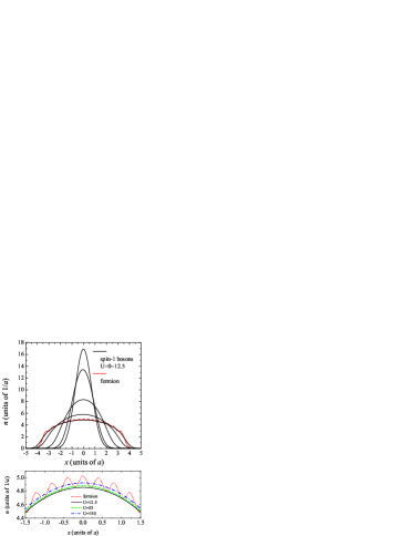
Figure 2: (Color Online) Density distribution of 1D trapped spin-1 bosons with $N=30$ and $P=0$. In the upper figure, five black solid lines from top to bottom are respectively for spinor bosons with $U=0,0.1,0.5,2,12.5$. Red dotted line is for non-interacting Fermions with mass $2m$. The lower figure shows the details of the peak density for even stronger interactions $U=12.5,25,150$. We observe a slightly rising of the peak after $U>12.5$.

Figure 3: Non-monotonicity of the central density $n^{(0)}$ of 1D trapped spin-1 bosons with increasing $U$ for $N=30$ and $P=0$. The exists a minimum value of $n^{(0)}$ at $U=12.5$ which is shown in the inset.

We now discuss the KS equations for the limiting cases of weak and strong interaction. When there is no interaction, KS equations correctly reduce to the 1D Schrödinger equation of simple harmonic oscillator. The Bose density profiles take the standard Gaussian shape

$$n_{1,2}\left(x\right)=\frac{N_{1,2}}{a\sqrt{\pi}}\exp\left(-x^{2}/a^{2}\right).$$ (45)

When the interaction is strong, the kinetic energies in (42) and (43) can be ignored, we have the TFA equations

$$\frac{1}{2}m\omega^{2}x^{2}+\mu_{1}\left(x\right) = \mu_{1}^{0},$$ (46)

$$\frac{1}{2}m\omega^{2}x^{2}+\frac{\mu_{2}\left(x\right)}{2} = \frac{\mu_{2}^{0}}{2}.$$ (47)

The values of $\mu_{1}^{0}$ and $\mu_{2}^{0}$ are fixed by the normalization conditions (33) and (34). Based on (46) and (47) Kuhn et al. give the ground state phase diagram and find that the singlet pairs and unpaired bosons may form a two-component Luttinger liquid in the strong coupling regime Kuhn2012 . When the interaction approaches infinitely strong, with the limit values of chemical potential (31, 32) and the normalization conditions (33, 34), we can solve (46, 47) to obtain the following half-ellipse-like density profiles

$$n_{1,2}\left(x\right)\approx\frac{\sqrt{2N_{1,2}-\left(x/a_{1,2}\right)^{2}}}{\pi a_{1,2}},$$ (48)

where $a_{1}=a$ and $a_{2}=\sqrt{\hbar/2m\omega}$. We see that the density of particle I is just that of $N_{1}$ noninteracting harmonically trapped fermions with mass $m$. The density of particles II is that of $N_{2}$ noninteracting fermions with mass $2m$. It shows that for infinitely strong interaction, the property of particles II approaches the TG gas of Bose-Bose pairs. Resorting to the Bose-Fermi mapping method Deuretzbacher2008 ; Girardeau2011 ; Girardeau1960 , we may map the densities of paired and unpaired components exactly to those of non-interacting Fermions

$$n_{1,2}\left(x\right)=\frac{1}{a_{1,2}\sqrt{\pi}}\exp\left(-x^{2}/a_{1,2}^{2}\right)\sum_{{l=0}}^{N_{1,2}-1}\frac{H_{l}^{2}\left(x/a_{1,2}\right)}{2^{l}l!},$$ (49)

where $H_{l}\left(x\right)$ is the Hermite polynomials.

III Numerical results

We introduce the interacting parameter $U=g/a\hbar\omega$. The space-dependent Lieb-Liniger parameter is expressed as $\gamma\left(x\right)=U/an\left(x\right)$. For the 1D spin-1 bosons with given $N$, $P$ and $U$, we present the numerical results for densities $n_{1}$ and $n_{2}$ of particle I and II obtained by solving the KS equations (42) and (43) with the iteration method. The ground state energy $E_{0}$ can be obtained via the relation (44). The numerical results are summarized in Figs. 2-10.

III.1 $P=0$ system

We first study the system with $N=30$ and $P=0$. In this fully paired case, the length, density and energy are in units of $a$, $1/a$ and $\hbar\omega$ respectively. Fig. 2 provides an understanding of how the density profiles change along with the interaction parameter for $U=0,0.1,0.5,2,12.5$ in the upper figure and $U=12.5,25,150$ in the lower figure. With the increasing of $U$, the total density profile varies from a standard Gaussian-like shape characterizing the distribution of non-interacting Bose gas to a half-ellipse shape indicating the distribution of non-interacting Fermi gas. Interestingly we find that the density profile of $N$ spin-1 bosons with mass $m$ for strongly interacting case e.g. $U=150$ overlaps that of $N/2$ noninteracting fermions with mass $2m$, except the emergence of the density oscillation in the Fermionic case. It means that for strong interaction all atoms in the anti-ferromagnetic spin-1 bosons are paired with each other, behaving like the TG gas of Boson pairs.

We surprisingly notice that the density profile does not change with the interaction parameter monotonically. The full tendency of the central density $n^{(0)}$ (density at the trap center $x=0$) can be seen in Fig. 3 and the inset shows in detail the non-monotonicity of $n^{(0)}$. We find that central density firstly decreases to a minimum value $n^{(0)}_{\min}=4.858/a$ at $U=12.5$ before reaching the constant central density of non-interacting fermions for large $U$. The result can be understood as the competition between the repulsive density-density interaction and the anti-ferromagnetic spin-exchange interaction with equal strength. The repulsive density-density interaction tends to increase the distance between bosons while the anti-ferromagnetic spin-exchange interaction leads essentially attraction between $s=\pm 1$ or $s=0$ bosons. For $U<12.5$, the prevailing repulsions among bosons tend to broaden them to wider space area and reduce the density of bosons in the trap center to a minimum. The anti-ferromagnetic effect is prominent for $U>12.5$ which contracts the bosons slightly.

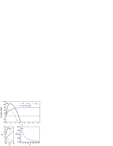
Figure 4: (Color Online) (a) Evolution of the ground state energy $E_{0}$ and all contributed energy terms of 1D trapped spin-1 bosons with increasing $U$ for $N=30$ and $P=0$. (b) the details of energies in the weak interaction regime. (c) the details of external potential energy.

Fig. 4 describes the evolution of the ground state energy $E_{0}$ and all contributed energy terms in Eq. (35) as a function of $U$. We can see the whole trend in (a) and the details in the mean field regime in (b). It shows that the kinetic energy $T^{ref}$ decreases slowly to a constant energy as the result of interactions restraining the movement of atoms. However, the external potential energy $E_{ext}$ increases due to the atoms occupy wider regime of the trap. In correspondence to the non-monotonicity of $n^{(0)}$, $E_{ext}$ shows non-monotonicity too, which can be seen clearly in Fig. 4(c). Close to the critical interaction value of $U=12.5$ for $n^{(0)}_{min}$ in Fig. (3c), $E_{ext}$ reaches its maximum $E_{ext}^{\max}=59.092\hbar\omega$ at $U=11.5$. But the non-monotonicity of $n^{(0)}$ doesn’t develop visible effects on other energy terms. Analogous to the ground state energy functional $e\left(\gamma,p=0\right)$ for homogeneous spin-1 bosons (see the upper panel of Fig. 1), the KS energy $E_{KS}$, i.e. the interaction energy, increases linearly in weak interaction regime and approaches its peak value $E_{KS}^{\max}=43.033\hbar\omega$ at $U=1.4$, corresponding to an axial L-L interaction parameter $\gamma^{(0)}=0.222$ ($\gamma$ at the trap center), followed by a monotonously decreasing in strong interaction regime. The contributions from $T^{ref}$, $E_{ext}$ and $E_{KS}$ together establish the ground state energy $E_{0}$ to increase to a maximum $E_{0}^{\max}=85.994\hbar\omega$ at $U=1.9$, corresponding to $\gamma^{(0)}=0.324$, and then decrease monotonously. We notice that the value $\gamma^{(0)}=0.324$ for $E_{0}^{\max}$ are close to $\gamma=0.4$ for the maximal $e$ in the upper panel of Fig. 1. We understand that the competition between the repulsion among paired bosons and the binding energy of the pair gives the peak of $E_{0}$ at $U=1.9$ for the same reason as in the homogeneous case, while that between the repulsive density-density interaction and the anti-ferromagnetic spin-exchange interaction gives the non-monotonicity of $n^{(0)}$ at $U=12.5$.

III.2 $P\neq 0$ system

For $P=1$, none of the bosons can form pair and the system reduces to the scalar Bose gas with density-density interaction $2g$, whose ground state properties have been studied by means of DFT in Ref. Hongmei2012 . With the increasing of $U$, the density distribution and energy of the system approach those of a single-component TG gas.

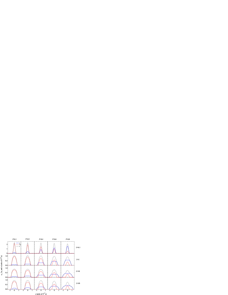
Figure 5: (Color Online) Density distributions of 1D trapped spin-1 bosons at $P=0.1,0.2,0.4,0.6,0.8$ (panels from left to right) and $U=0.1,2,10,50$ (panels from top to bottom). Blue solid lines denote the densities for polarized particles $n_{1}$, red dashed lines denote the densities for paired bosons $2n_{2}$, and black dotted lines denote the total densities $n$.

Here we study the interesting situation of a partially polarized spinor gas with total polarization $0<P<1$. In this case the length, density and energy are in units of $N^{1/2}a$, $N^{1/2}/a$ and $\hbar\omega$ respectively. In Fig. 5 we illustrate the density of polarized particles $n_{1}$ (blue solid lines), density of paired bosons $2n_{2}$ (red dashed lines) and the total density $n$ (black dotted lines) for various polarization $P=0.1,0.2,0.4,0.6,0.8$ (the figures in the columns from left to right) and interaction $U=0.1,2,10,50$ (the figures in the rows from up to down). Horizontal view shows that the density profile $n_{1}$ expands gradually with the increasing of $P$ accompanied by the corresponding shrinking of $2n_{2}$. These two densities together result in a slightly decreasing of the peak density $n^{(0)}$ for increasing $P$. An analysis of vertical scope for increasing interaction parameter $U$ (note that we use different vertical axis scale in the weak interaction case $U=0.1$) tells us that the density $2n_{2}$ changes smoothly from the Gaussian distribution of non-interacting Bose gas to the half-ellipse distribution of TG gas of Bose-Bose pairs. The density peak is located in the center of the trap for all interaction strengths. The behavior of density $n_{1}$ is, however, a little complicated. Though $n_{1}$ shows Gaussian distribution for weak interaction ($U=0.1$), bosons of Particle I tend to occupy wider space and start to be excluded from the trap center for intermediate interaction ($U=2,10$). The single peak profile of $n_{1}$ changes into the double-peak distribution. This reminds us the partially phase separation of Bose-Fermi mixture with equal mass and equal repulsive interaction Imambekov2006 ; Hongmei2012 . In our case, the phase separation of paired and unpaired bosons occurs in the system, i.e. the core area of the 1D spinor gas is filled with the mixture of paired and unpaired bosons and in the outer region we find either polarized bosons for $P>0.2$ or paired bosons for $P<0.2$. For even stronger interaction ($U=50$), the peak of $n_{1}$ returns back to the trap center and the density profile $n_{1}$ approaches the half-ellipse distribution of TG gas. Nevertheless the evidence of phase separation becomes more prominent in the strongly interaction case.

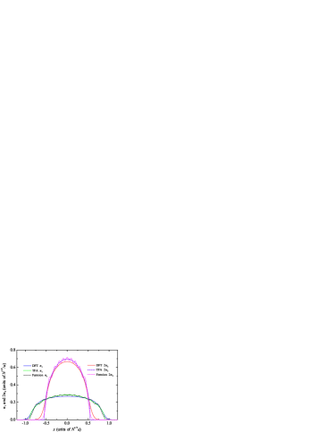
Figure 6: (Color Online) Comparison of the density distribution of 1D trapped spin-1 bosons at $P=0.4$ in the case of strong interaction. The results for both $n_{1}$ and $2n_{2}$ are from DFT for $U=50$ (solid lines), TFA for $U=+\infty$ (dashed lines), and $N=30$ non-interacting fermions (dotted lines), respectively. Clear evidence is observed for the phase separation and in this case the surrounding wings are composed of polarized particles. The radius of vanishing density from DFT is obviously larger than the TFA result.

As a result the total density $n$ shows the overall Gaussian distribution showing a fully mixing phase of $n_{1}$ and $2n_{2}$ at weak interaction ($U=0.1$). When the interaction increases, we find a bi-modal distribution of the total density with particle II imposed on the top of particle I, i.e. the mixed core of particles I and II is surrounded by two wings composed of solely polarized bosons for large $P$ and large $U$ (see the several right-down panels of Fig. 5). Take the $P=0.4$ case as an example. We compare the density plots for the two components in Fig. 6. The solid lines are our DFT results from the iteration solution of the KSE Eqs. (42) and (43), while the dashed lines are analytical TFA results Eq. (48) for infinitely strong interaction. Also shown are the densities of non-interacting fermions Eq. (49) according to the Bose-Fermi mapping (dotted lines) for $N=30$. We identify readily the density oscillations with 12 peaks in the polarized component $n_{1}$ in the TG limit and 9 peaks in the paired component $n_{2}$ representing the TG gas of 9 pairs of bosons.

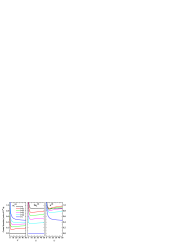
Figure 7: (Color Online) Evolution of central densities $n_{1}^{(0)}$, $n_{2}^{(0)}$ and $n^{(0)}$ (panels from left to right) of trapped spin-1 bosons with increasing interaction parameter $U$. Non-monotonicity is seen for all partially polarized cases $0<P<1$.

An interesting observation is the non-monotonicity of the central density value $n^{(0)}$ which already occurs in the fully paired case $P=0$. We take a close look at the rise-and-fall of the peak values for polarized bosons, paired bosons, and the total density. Fig. 7 shows the evolution of central densities with increasing interaction parameter $U$ for different $P$. For the central density of polarized particles $n_{1}^{(0)}$, we find it is a constant zero at $P=0$ since there are no Particle I in the gas and a monotonically decreasing curve at $P=1$ corresponding to the scalar Bose gas. In all partially polarized case $0<P<1$, the peak values rapidly decrease to a minimum $n_{1\min}^{(0)}$ and then gradually approach to a constant for strong interaction. The minimum is seen to move toward the stronger interaction direction with increasing $P$ and finally disappear for $P=1$. On the contrary, the central density of paired particles $n_{2}^{(0)}$ is a constant zero at $P=1$ since there are no paired bosons in the gas and a seemingly monotonically decreasing curve at $P=0$ corresponding to the fully paired bosons. Yet we know from the result of $P=0$ in Fig. 3 there indeed exists a minimum due to the competition between the density interaction and spin exchange. The competition persists here for all partially polarized cases, leading to similar shallow low-lying areas, whose minimum is seen to move toward the weaker interaction direction with increasing $P$ as shown in the middle panel of Fig. 7. The total central density comes from the combination of these two terms $n^{(0)}=n_{1}^{(0)}+2n_{2}^{(0)}$. The right panel shows that the minimum hollow for the total central density remains for all partially or fully polarized cases $0\leq P<1$ and the tail of $n^{(0)}$ in strong interaction limit firstly goes up slightly followed by a nearly linear decreasing for increasing $P$. This non-monotonicity of the total central density in strong interaction case ($U=50$) is depicted in detail in Fig. 8 for increasing $P$, together with the monotonic behavior of the central density for polarized bosons (down-ward) and that for paired bosons (up-ward). The results from DFT are compared with the analytical curves from the TFA. We find that in the case of $U=50$ the central densities for all polarized situation are already very close to the limiting value in TFA, which are obtained from eq. (48) as

$$n_{1}^{(0)} = \frac{\sqrt{2NP}}{\pi a},$$

$$2n_{2}^{(0)} = \frac{2\sqrt{2N(1-P)}}{\pi a},$$

$$n^{(0)} = \frac{\sqrt{2N}(\sqrt{P}+2\sqrt{1-P})}{\pi a}.$$ (50)

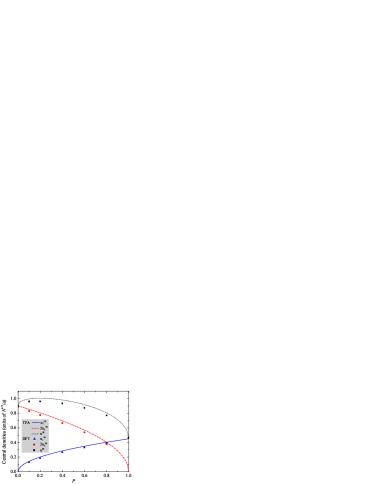
Figure 8: (Color Online) Central densities $n_{1}^{(0)}$, $n_{2}^{(0)}$ and $n^{(0)}$ as a function of $P$ for 1D trapped spin-1 bosons in the strong interaction case. The results of DFT for $U=50$ denoted by lines are in agreement with those in TFA for $U=+\infty$ denoted by symbols.

We may go further into the detailed quantum phases of the spinor gas by defining the radii of the vanishing densities for the two components. Fig. 9 shows the phase diagram as a function of the global polarization $P$ for $U=50$, where the axial radii of the ensemble of the polarized and paired components are extracted from the numerical result of the density profiles from the KSE. Without loss of generality, we set the threshold values of the vanishing scaled density as $0.02$ in the numerical simulation. The intersection of these two radii gives the boundaries which divided the phase plane into three quantum phases: spin-singlet-paired bosons S, ferromagnetic spin-aligned bosons F, mixed phase of the pairs and unpaired bosons M, while V stands for the vacuum. At low polarization a partially polarized region forms at the trap center, the radius of which increases with increasing polarization. At a critical polarization $P_{c}$, the partially polarized region extends to the edge of the cloud. When the polarization increases further, the edge of the cloud becomes fully polarized. This process can be evidently seen in the lowest panels in Fig. 5. Together shown in Fig. 9 are the theoretical results in TFA. According to eqs. (48), the radii of the vanishing densities are calculated as

$$R_{1} = \sqrt{2NP}a,$$

$$R_{2} = \sqrt{\frac{N(1-P)}{2}}a$$ (51)

When the two radii equal to each other, we find the critical polarization is $P_{c}=0.2$ and the critical radius is $R_{c}=0.63$. The DFT results for the radii are apparently larger than the TFA estimation for both polarized and fully paired bosons, which can be understood easily from the extension of the tail of the density profile into outer region (see Fig. 6). Energetically this extension is due to the kinetic term neglected in TFA. The critical polarization is in agreement with the TFA crossing at slightly higher polarization $P_{c}\sim 0.23$ and larger radius $R_{c}\sim 0.73$.

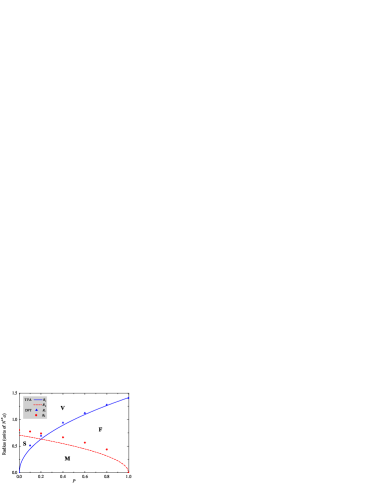
Figure 9: (Color Online) R-P phase diagram of 1D trapped spin-1 bosons in terms of the scaled density radii $R$ as the functions of total polarization $P$. Three quantum phases are identified: spin-singlet-paired phase (S), ferromagnetic spin-aligned phase (F) and mixed phase of the pairs and unpaired bosons (M). V stands for vacuum. The results of DFT for $U=50$ ($n_{1}$, $2n_{2}<0.02$ are considered as vanishing scaled densities) and analytical results in TFA for $U=+\infty$ are compared.

The phenomena of phase separation at strong interaction is consistent with the results of Ref. Kuhn2012 . There they gave the ground state phase diagram according to the evolvement of Thomas-Fermi radii of $n_{1}$ and $n_{2}$ along with $P$ by the means of TBA for strong interaction case. Our results, on the other hand, are valid for systems in the whole interaction regime. Interestingly we found the double-peak structure of the density of polarized bosons at intermediate interaction, which is elusive from the method in Kuhn2012 . In a seminal experiment on spin-imbalanced 1D two-component Fermi gas Liao2010 , phase separation of the two-spin mixture of ultracold ⁶Li atoms trapped in an array of 1D tubes is reported. The partially polarized core is surrounded by wings which are composed of either a paired or a polarized Fermi gas depending on the polarization $P$. The pair mechanism in spinor gas is challenged by the density repulsive interaction, which makes the phase separation more complicated.

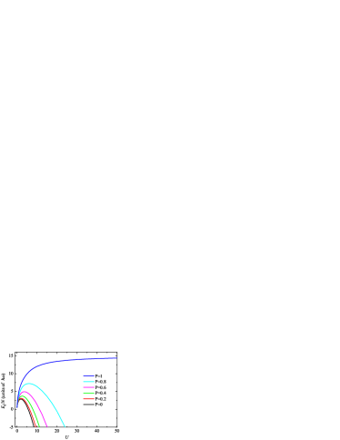
Figure 10: (Color Online) The ground state energy per atom of 1D trapped spin-1 bosons as functions of $U$ for different $P$. The lines are for P=0,0.2,0.4,0.6,0.8,1 from bottom to top.

Finally, just as $e(\gamma,p)$ shows the interaction dependence for various polarizations in the homogeneous case and $E_{0}$ in Eq. (44) gives the change with interaction in the fully paired case, we illustrate in Fig. 10 the evolution of ground state energies $E_{0}$ per atom along with interaction $U$ and total polarization $P$ in all partially polarized cases. The black solid line for $P=0$ here repeats the result of $E_{0}$ in Fig. 4. The fully polarized $P=1$ system is equivalent to the 1D trapped repulsive scalar bosons in Hongmei2012 and $E_{0}$ increases monotonously and approach the ground state energy of non-interacting fermion system. The energy for partially polarized system with $0<P<1$ interpolates between these two extremes, i.e., the positive energy terms including the kinetic, potential and density-density repulsive interactions together compete with the negative binding energy in the anti-ferromagnetically paired bosons, giving rise to the non-monotonically dependence of the energy on the interaction parameter $U$. In the weak interaction case, the repulsive interaction is prominent so that $E_{0}$ increases along with $U$. In the strong interaction case, $E_{0}$ decreases because the repulsive energy slowly increases to a constant whereas the binding energy goes downward parabolically. Larger polarization destroys the Bose-Bose pairs one by one, which diminishes the effect of pairing binding energy and finally leads to the monotonic behavior of $E_{0}$ for $P=1$.

IV Conclusion

In conclusion, using DFT we study the density distribution and energy of the 1D harmonically trapped spin-1 bosons in the ground state. We numerically solve the KSEs based on LDA and the solution of Bethe ansatz. The results show that the competition between the repulsive density-density interaction and antiferromagnetic spin-exchange interaction results in complicated density distributions and energy evolutions along with the interaction parameter. We found a non-monotonic behavior in the central densities of both spin-singlet paired and polarized bosons. Some polarized bosons are repelled out of the trap center in the intermediate interaction region, showing the double-peak structure of density profiles. The total density exhibits a bi-modal distribution with paired bosons imposed on the top of polarized bosons. The phenomena of phase separation occurs for strong interaction with the partially polarized core surrounded by wings which are composed of either paired bosons or polarized bosons depending on the polarization $P$. We give the R-P phase diagram at strong interaction and find that the critical polarization $P_{c}$ in DFT is slightly larger than the TFA result. Although we treat with an integrable model with equal repulsive density interaction and antiferromagnetic spin-exchange, the results do shed some light on the relativistic spinor gases. We speculate that the new quantum phases investigated here could be probed in experiment by in situ imaging, analogously to the 1D trapped Fermi gas Liao2010 .

- (1) Y. Kawaguchi and M. Ueda, Phys. Rep. 520, 253 (2012).
- (2) D. M. Stamper-Kurn and M. Ueda, arXiv:1205.1888.
- (3) M. A. Cazalilla, R. Citro, T. Giamarchi, E. Orignac, and M. Rigol, Rev. Mod. Phys. 83, 1405 (2011).
- (4) X.-W. Guan, M. T. Batchelor and C. Lee, arXiv:1301.6446.
- (5) W. Zhang and L. You, Phys. Rev. A 71, 025603 (2005).
- (6) Y. Hao, Y. Zhang, J. Q. Liang, and S. Chen, Phys. Rev. A 73, 053605 (2006).
- (7) J. Cao, Y. Jiang, and Y. Wang, Europhys. Lett. 79, 30005 (2007).
- (8) F. Deuretzbacher, K. Fredenhagen, D. Becker, K. Bongs, K. Sengstock, and D. Pfannkuche, Phys. Rev. Lett. 100, 160405 (2008).
- (9) M. D. Girardeau, Phys. Rev. A 83, 011601(R) (2011).
- (10) F. H. L. Essler, G. V. Shlyapnikov, and A. M. Tsvelik, J. Stat. Mech. 02, P02027 (2009).
- (11) J. Y. Lee, X.-W. Guan, M. T. Batchelor, and C. Lee, Phys. Rev. A 80, 063625 (2009).
- (12) C. C. N. Kuhn, X. W. Guan, A. Foerster, and M. T. Batchelor, Phy. Rev. A 85, 043606 (2012); ibid. 86, 011605(R) (2012).
- (13) Y. Liao, A. Rittner, T. Paprotta, W. Li, G. Patridge, R. Hulet, S. Baure, and E. Mueller, Nature (London) 467, 567 (2010).
- (14) S. De, D. L. Campbell, R. M. Price, A. Putra, B. M. Anderson, and I. B. Spielman, arXiv:1211.3127.
- (15) A. Vinit, E. M. Bookjans, C. A. R. Sá de Melo, and C. Raman, arXiv:1212.2233.
- (16) D. M. Stamper-Kurn, M. R. Andrews, A. P. Chikkatur, S. Inouye, H.-J. Miesner, J. Stenger, and W. Ketterle, Phys. Rev. Lett. 80, 2027 (1998).
- (17) H.-J. Miesner, D. M. Stamper-Kurn, J. Stenger, S. Inouye, A. P. Chikkatur, and W. Ketterle, Phys. Rev. Lett. 82, 2228 (1999).
- (18) M. R. Matthews, B. P. Anderson, P. C. Haljan, D. S. Hall, C. E. Wieman, and E. A. Cornell, Phys. Rev. Lett. 83, 2498 (1999).
- (19) M. D. Barrett, J. A. Sauer, and M. S. Chapman, Phys. Rev. Lett. 87, 010404 (2001).
- (20) A. Crubellier, O. Dulieu, F. Masnou-Seeuws, M. Elbs, H. Knockel, and E. Tiemann, Eur. Phys. J. D 6, 211 (1999).
- (21) E. G. M. van Kempen, S. J. J. M. F. Kokkelmans, D. J. Heinzen and B. J. Verhaar, Phys. Rev. Lett. 88, 093201 (2002).
- (22) T. Ohmi and K. Machida, J. Phys. Soc. Jpn. 67, 1822 (1998).
- (23) T.-L. Ho, Phys. Rev. Lett. 81, 742 (1998).
- (24) M. Koashi and M. Ueda, Phys. Rev. Lett. 84, 1066 (2000).
- (25) C. K. Law, H. Pu, and N. P. Bigelow, Phys. Rev. Lett. 81, 5257 (1998).
- (26) H. Pu, C. K. Law, S. Raghavan, J. H. Eberly, and N. P. Bigelow, Phys. Rev. A 60, 1463 (1999).
- (27) W. Zhang, D. L. Zhou, M-S. Chang, M. S. Chapman, and L. You, Phys. Rev. A 72, 013602 (2005).
- (28) J. Zhang, T. Li, and Y. Zhang, Phys. Rev. A 83, 023614 (2011).
- (29) T.-L. Ho and S.-K. Yip, Phys. Rev. Lett. 84, 4031 (2000).
- (30) E. J. Mueller, T.-L. Ho, M. Ueda, and G. Baym, Phys. Rev. A 74, 033612 (2006).
- (31) J. Zhang, Z.F. Xu, and L. You, Y. Zhang, Phys. Rev. A 82, 013625 (2010).
- (32) M. Greiner, I. Bloch, O. Mandel, T. W. Hänsch, and T. Esslinger, Phys. Rev. Lett. 87, 160405 (2001).
- (33) H. Moritz, T. Stöferle, M. Köhl, and T. Esslinger, Phys. Rev. Lett. 91, 250402 (2003).
- (34) B. Paredes, A. Widera, V. Murg, O. Mandel, S. Fölling, I. Cirac, G. V. Shlyapnikov, T. W. Hänsch, and I. Bloch, Nature (London) 429, 277 (2004).
- (35) T. Kinoshita, T. Wenger, and D. S. Weiss, Science 305, 1125 (2004).
- (36) E. Haller, M. Gustavsson, M. J. Mark, J. G. Danzl, R. Hart, G. Pupillo, and H. C. Nägerl, Science 325, 1224 (2009).
- (37) M. Olshanii, Phys. Rev. Lett. 81, 938 (1998); T. Bergeman, M.G. Moore, and M. Olshanii, ibid. 91, 163201 (2003).
- (38) T. Bergeman, M. G. Moore and M. Olshanii, Phy. Rev. Lett 91, 163201 (2003).
- (39) S. Sinha and L. Santos, Phy. Rev. Lett 99, 140406 (2007).
- (40) E. H. Lieb and W. Liniger, Phys. Rev. 130, 1605 (1963).
- (41) C. N. Yang , Phys. Rev. Lett. 19, 1312 (1967).
- (42) C. N. Yang , Phys. Rev. 168, 1920 (1968).
- (43) J. N. Fuchs, A. Recati, and W. Zwerger, Phys. Rev. Lett. 93, 090408 (2004).
- (44) A. Imambekov and E. Demler, Phys. Rev. A 73, 021602 (R) (2006); Ann. Phys. 321, 2390 (2006).
- (45) A. Imambekov, M. Lukin, and E. Demler, Phys. Rev. A 68, 063602 (2003).
- (46) B. Sutherland, Phys. Rev. Lett. 20, 98 (1968).
- (47) M. Girardeau, J. Math. Phys. 1, 516 (1960).
- (48) P. Hohenberg and W. Kohn, Phys. Rev. 136, B864 (1964); W. Kohn and L. J. Sham, ibid. 140, A1133 (1965); W. Kohn, Rev. Mod. Phys. 71, 1253 (1999).
- (49) R. M. Dreizler and E. K. U. Gross, Density Functional Theory (Springer, Berlin, 1990).
- (50) G. S. Nunes, J. Phys. B 32, 4293 (1999); A. Banerjee and M. P. Singh, Phys. Rev. A 73, 033607 (2006); N. Argaman and Y. B. Band, ibid. 83, 023612 (2011).
- (51) Y. E. Kim and A. L. Zubarev, Phys. Rev. A 67, 015602 (2003).
- (52) A. P. Albus, F. Illuminati, and M. Wilkens, Phys. Rev. A 67, 063606 (2003).
- (53) P. N. Ma, S. Pilati, M. Troyer, and X. Dai, Nature Phys. 8, 601 (2012).
- (54) J. Brand, J. Phys. B 37, S287 (2004).
- (55) Y. Hao and S. Chen, Phys. Rev. A 80, 043608 (2009).
- (56) G. E. Astrakharchik, D. Blume, S. Giorgini, and L. P. Pitaevskii, Phys.Rev. Lett. 93, 050402 (2004); Y. E. Kim and A. L. Zubarev, Phys. Rev. A 70, 033612 (2004); R. J. Magyar and K. Burke, ibid. 70, 032508 (2004).
- (57) G. Xianlong, M. Polini, R. Asgari, and M. P. Tosi, Phys. Rev. A 73, 033609 (2006); G. Xianlong and R. Asgari, ibid. 77, 033604 (2008); G. Xianlong, M. Polini, D. Rainis, M.P. Tosi, and G. Vignale, Phys. Rev. Lett. 101, 206402 (2008).
- (58) H. Wang, Y. Hao and Y. Zhang, Phy. Rev. A 85, 053630 (2012).