Process optimized quantum cloners via semidefinite programming

Abstract

We apply semidefinite programming for designing 1 to 2 symmetric qubit quantum cloners. These are optimized for the average fidelity of their joint output state with respect to a product of multiple originals. We design 1 to 2 quantum bit cloners using the numerical method for finding completely positive maps approximating a nonphysical one optimally. We discuss the properties of the so-designed cloners.

I Introduction

A quantum process describes what can happen to a physical system when its state changes. Mathematically it is a mapping from the set of the initial states of the system to that of its final states. Quantum mechanics provides well-defined limitations to the process to be physically realistic. Apart from having to be linear, positive and trace preserving, it should be completely positive, too. This is an important constraint in the design of any quantum information processing apparatus.

Quantum cloning is a celebrated counterexample of a physically realistic process, producing identical copies of a physical system in a given unknown quantum state. This mapping is not even linear, hence it is unfeasible physically. Of course, if something is unfeasible, it can still be approximated, as described first in Ref. PhysRevA.54.1844 . Since that, the topic of cloning achieved a broad coverage in the literature (see Ref. cloning for a review), including the calculation of achievable fidelities and several designs of particular schemes for cloning. These designs of optimal cloners are based on some intuitive physical ideas, which makes them well understandable and gives a hint for laboratory interpretation.

It is also known that the methods of semidefinite programming in operations research makes it possible to find completely positive maps ideally approximating nonphysical ones. In Ref. koenraad , where this idea was introduced, an example is given which is a universal shifter PhysRevA.63.032304 ; PhysRevA.64.062310 ; PhysRevA.64.032301 , a nonlinear operation on a single qubit. Besides of the valuable analytical techniques, Ref koenraad . gives a complete numerical recipe to design arbitrary operations.

In the present work we utilize this numerical technique in order to analyze the design of 1 to 2 quantum bit cloners. It turns out that partly due to the nature of the optimization method, the so designed cloner is not optimized with respect to the fidelity of the clones to the input state, but the average fidelity of the whole (two-qubit output) with respect to a tensor product of two copies of the original. For universal symmetric quantum cloners, that is, those which work for an arbitrary input qubit state, it was shown by Werner Werner and Keyl and Werner KeylWerner in a much more general context that optimizing the fidelity of the two qubit output state is equivalent to that of optimizing the fidelity of the two cloners. For phase-covariant cloners, that is, for which the input state is restricted to those on a main circle of the Bloch sphere, the two aspects are not equivalent. The design of the phase covariant cloners for qubits and qutrits is studied in detail in the paper of D’Ariano and Macchiavello in Ref. DAriano . Even though the existence and some properties are covered by these papers partly, we the use different, numerical approach, an application of the general method in Ref koenraad . This provides us with easily applicable mappings and demonstrates the power of semidefinite programming in this field. It is also interesting to compare the maps we have found with the universal covariant quantum cloner (UCQC) circuit designed by Braunstein et al. PhysRevA.63.052313 .

This paper is organized as follows. In Section II we review the method for finding optimal CP approximations of nonphysical maps via semidefinite programming, and discuss its application to quantum cloning, introducing the notion of process optimized cloners. In Section III we present and discuss our particular results. In Section IV conclusions are drawn and an outlook is provided.

II Design method

In this Section we first briefly summarize the method for designing CP maps via semidefinite programming, which optimally approximate an unphysical map. This is entirely described in detail in Ref. koenraad , we just repeat the main ideas here for sake of self-consistency. In the second subsection, the application of this method to the design of quantum cloners is discussed, which leads us to the concept of process-optimized cloners.

II.1 Optimizing CP maps via semidefinite programming

Consider a quantum operation $\mathcal{S}:\mathcal{B}(\mathcal{H_{\text{in}}})\mapsto\mathcal{B}(\mathcal{H_{\text{out}}})$, mapping states in the Hilbert space $\mathcal{H}_{\text{in}}$ to those of $\mathcal{H}_{\text{out}}$, $\mathcal{B}$ denoting the set of density operators on the given Hilbert space. In order to be physically realistic, the mapping $\mathcal{S}$ has to be a linear, completely positive (CP) trace preserving one. In some cases, however, one might want to at least approximately realize processes which are non-CP, or not even linear. Examples include the quantum shifter discussed in Refs. PhysRevA.63.032304 ; PhysRevA.64.062310 ; PhysRevA.64.032301 and quantum cloning studied here, etc.

So we consider an ideal process $\mathcal{S}_{\text{id}}$ which is arbitrary, and we seek a realistic (linear, trace-preserving, CP) map $\mathcal{S}$ which approximates $\mathcal{S}_{\text{id}}$ to the highest extent. This latter should be quantified somehow. In order to do so, consider an input set $T\subset\mathcal{B}(\mathcal{H_{\text{in}}})$, containing the states for which we would like our approximate process to be optimal. (This possible restriction might be of some use, it enables us, for instance, to consider non-universal quantum cloners in this framework.) We assume that it is possible to integrate over $T$ according to a suitable measure, this will be denoted by $\int_{T}dT$. The quantity to be optimized will be

$$\mathcal{F}=\int_{T}dT\left(\mathop{\mbox{tr}}\sqrt{\sqrt{\mathcal{S}_{\text{id}}(\varrho)}\mathcal{S}(\varrho)\sqrt{\mathcal{S}_{\text{id}}(\varrho)}}\right)^{2},\quad(\varrho\in T),$$ (1)

the fidelity of the output state of the realistic process with respect to that of the desired ideal process, averaged over the considered input states. We shall term this as process fidelity in what follows. In the special case when the set $\{\mathcal{S}_{\text{id}}(\varrho)|\varrho\in T\}$ contains pure states only, that is, we expect the ideal process to map the states of the target space to pure states only, the fidelity in Eq. (1) simplifies to

$$\mathcal{F}=\int_{T}dT\mathop{\mbox{tr}}\left(\mathcal{S}_{\text{id}}(\varrho)\mathcal{S}(\varrho)\right),\quad(\varrho\in T),$$ (2)

as $\mathcal{S}_{\text{id}}(\varrho)$ is a one-dimensional projector. Throughout this paper we shall treat the latter case only, as we are interested in cloning of pure states, which ideally results in products of pure states.

According to Ref. koenraad , this optimization can be performed in the following way. We consider a fixed basis on both the input and output Hilbert spaces. $\mathcal{S}$ is sought for in its Choi-representation, in which it is represented by a Hermitian, positive semidefinite operator $X$ acting on $\mathcal{H}_{\text{in}}\otimes\mathcal{H}_{\text{out}}$, and the relation of the output state to that of the input reads

$$\mathcal{S}(\varrho)=\mathop{\mbox{tr}}_{\mathcal{H}_{\text{in}}}\left(\left(\varrho^{T}\otimes\hat{1}\right)X\right),$$ (3)

where $T$ means ordinary (not Hermitian) transpose in the fixed basis, and $\hat{1}$ stands for the identity operator. In this representation the process fidelity in Eq. (1) of the process can be expressed as

$$\mathcal{F}=\mathop{\mbox{tr}}\left(XR\right),$$ (4)

where

$$R=\int_{T}dT\varrho^{T}\otimes\mathcal{S}_{\text{id}}(\varrho).$$ (5)

The input of the optimization is the matrix $R$ encoding all the relevant information on the set $T$ and the process $\mathcal{S}$ to be approximated. The output will be the Choi matrix $X$ of the ideal process and the maximum value $\mathcal{F}^{\ast}$ of the process fidelity. Again note that for Eq. (4) to hold, $\mathcal{S}_{\text{id}}(\varrho)$ has to be a pure state, that is, a one-dimensional projector.

In the next step we fix two orthonormal bases: $\sigma$ and $\tau$, in the linear space of the Hermitian matrices over $\mathcal{H}_{\text{in}}$ and $\mathcal{H}_{\text{out}}$ respectively. Assuming $\dim\mathcal{H}_{\text{in}}=\dim\mathcal{H}_{\text{out}}=d$, we have $d^{2}$ basis elements. We chose $\sigma_{0}$ and $\tau_{0}$ to be proportional to the identity matrix, whereas the other basis elements, indexed with positive integers, should be traceless. For $d=2$ the Pauli matrices, for $d=3$ the Gell-Mann matrices, while for higher dimensions, generalized Pauli matrices are a suitable choice.

As derived in Ref. koenraad , one can construct the following semidefinite program (in dual form, that is, in the form of matrix inequalities) to optimize $\mathcal{F}$ in Eq. (2):

maximize $$p=-c^{T}x$$

subject to $$F_{0}+\sum_{\tilde{i}}x_{\tilde{i}}F_{\tilde{i}}\geq 0,$$ (6)

where $\geq 0$ means positive semidefiniteness, $F_{0}=\frac{1}{d}\hat{1}$, and

$$F_{\tilde{i}}=\sigma_{j(\tilde{i})}\otimes\tau_{k(\tilde{i})},$$ (7)

and the indices $1\leq\tilde{i}\leq d^{2}(d^{2}-1)$ are chosen so that the $j(\tilde{i})$-s take all the possible values from $0$ to $d^{2}$, while the $k(\tilde{i})$-s take all the possible values from $1$ to $d^{2}$, and the relation of the possible $(j,k)$ pairs and $\tilde{i}$-s is bijective. The vector $x$ is the one to be found while the constant coefficients $c$ in Eq. (II.1) are defined as

$$c_{\tilde{i}}=-\mathop{\mbox{tr}}\left(RF_{\tilde{i}}\right).$$ (8)

Note that these coefficients encode the matrix $R$ of Eq. (5), which, on the other hand, encodes all the information about the process $\mathcal{S}_{\text{id}}$ to be approximated as well as on the target set $T$. Having found the optimum $p^{\ast}$ of the semidefinite program in Eq. (II.1), the optimal fidelity is given by

$$F^{\ast}=p+\frac{1}{d},$$ (9)

whereas the Choi matrix of the process realizing it reads, in terms of the vector $x$ corresponding to the optimum:

$$X_{\text{opt}}=\sum_{\tilde{i}}x_{\tilde{i}}F_{\tilde{i}}+\frac{1}{d}\hat{1}.$$ (10)

This is the recipe derived in Ref. koenraad for finding optimal approximate realizations of quantum processes. It can be used numerically to design approximate processes. As it requires a semidefinite solver which is capable of handling Hermitian (complex) matrices, SeDuMi S98guide appears to be a proper choice. To invoke it for a semidefinite program formulated in Eq. (II.1), it is very convenient to use the Matlab package of T. Cubitt quantinf , which we have done in order to develop our Matlab code producing the results described in what follows.

II.2 Application for quantum cloning

Consider the case of quantum cloning. In general we are given $m$ copies of a physical system, all in the same identical quantum state, say $|\Psi\rangle$. We would like to obtain $n>m$ systems, so that the state of each system is closest in fidelity to $|\Psi\rangle$. In the simplest case, discussed in what follows, that of the $1\to 2$ qubit cloners, we have a single qubit in state $|\Psi\rangle$, and we obtain two copies in states $\varrho_{1}$ and $\varrho_{2}$ so that their fidelity with respect to $|\Psi\rangle$ is maximal. If we want a symmetric cloner, for which both fidelities are maximal, we have a problem characterized by two objective functions. This is not suitable for the recipe described in the previous section. Even if we consider the fidelity of the two clones to be equal, it is not the kind of problem solved above with semidefinite programming.

What we might consider instead is the following. Take the system in state $|\Psi\rangle$, and an ancilla, in an arbitrary state, say $|0\rangle$. The target set $T$ shall be the set for which we are considering to plan a cloner, e.g. for a universal qubit cloner, the surface of the Bloch-sphere, but we may consider restricted input sets. Then carry out the procedure so that the ideal process should be $|\Psi\rangle\otimes|0\rangle\to|\Psi\rangle\otimes|\Psi\rangle$, which is obviously unfeasible due to the no-cloning theorem. The fidelity $\mathcal{F}$ considered in this optimization is, however, not the same as optimizing the fidelity of the clones.

One may realize that it might be even a different problem. Namely, we do not look for a process which produces two identical copies which resemble the original to the highest extent, but we look for a process which produces the product of the two originals to the highest extent. For a symmetric $1\to 2$ cloner, the fidelity of each clone to the original is considered, which will be termed as cloning fidelity in what follows. The cloners we design here, on the other hand, are optimal with respect to the process fidelity, hence, we shall call them process-optimized cloners.

Process-optimized cloners, as it was mentioned in the introduction, were studied in the early literature of cloning. As it appears that this kind of optimization is suitable for SDP, it is still of some interest to study the actual designs which SDP provides automatically.

III Process-optimized quantum cloner designs

In this Section we describe our results regarding process-optimized $1\to 2$ qubit cloners designed the above-described method. The numerical results are summarized in Table 1.

Cloner	$F_{C}$	$F_{P}$	$C$	$H_{\text{clone}}$	$H_{\text{out}}$
UCQC, symmetric mode	$\frac{5}{6}\approx 0.83333$	$\frac{2}{3}\approx 0.66667$	$\frac{1}{3}\approx 0.33333$	$0.65002$	$0.91830$
universal, opt. for ancilla: $|0\rangle$, used ancilla: $|0\rangle$	0.83333	0.66667	0.33333	0.65002	0.91830
universal, opt. for ancilla: $\frac{1}{2}\hat{1}$, used ancilla: $\frac{1}{2}\hat{1}$	0.83333	0.66667	0.33333	0.65002	0.91830
universal, opt. for ancilla: $|0\rangle$, used ancilla: $\frac{1}{2}\hat{1}$	0.66667	0.45833	0.00000	0.91830	1.78434
universal, opt. for ancilla: $\frac{1}{2}\hat{1}$, used ancilla:$|0\rangle$	0.83333	0.66667	0.33333	0.65002	0.91830
equator, opt. for ancilla: $|0\rangle$, used ancilla: $|0\rangle$	0.83333	0.75000	0.33333	0.65002	0.65002
equator, opt. for ancilla: $\frac{1}{2}\hat{1}$, used ancilla: $\frac{1}{2}\hat{1}$	0.83333	0.75000	0.33333	0.65002	0.65002
equator, opt. for ancilla: $|0\rangle$, used ancilla: $\frac{1}{2}\hat{1}$	0.66667	0.50000	0.00000	0.91830	1.70058
equator, opt. for ancilla: $\frac{1}{2}\hat{1}$, used ancilla: $|0\rangle$	0.83333	0.75000	0.33333	0.65002	0.65002

Table 1: Input-state independent parameters of the designed cloners. The most relevant issues are typeset in bold.

III.1 The universal covariant quantum cloner

First we calculate the properties of the qubit-version of the universal covariant quantum cloner (UCQC) designed by Braunstein et al. PhysRevA.63.052313 We use this particular cloner design as a benchmark for those designed by us. We use this cloner since it is known to be optimal and it is a particular circuit so all of its properties can be investigated.

The quantum logic network for the UCQC is depicted in Fig. 1.

Figure 1: The quantum logic network for the universal quantum cloner of Ref. PhysRevA.63.052313 , used here as a benchmark. Input ports are to to left, whereas the outputs to the right.

The “circuitry” consists of four controlled NOT gates. We do not consider all of its capabilities here, just one very particular case: If a qubit in a quantum state $|\Psi_{\text{in}}\rangle$ to be cloned impinges on port 1, while the so-called program state is chosen to be

$$|\Psi^{\text{prog}}\rangle=\frac{1}{\sqrt{6}}\left(2|0\rangle|0\rangle+|0\rangle|1\rangle+|1\rangle|1\rangle\right),$$ (11)

then in the outputs 1 and 2 there will be two identical clones of the state to be cloned. (Port 3 will hold a state related to the input, it will be omitted). Moreover, their density matrix will be the mixture of the state to be cloned and a complete mixture. This case (i.e. the symmetrical mode of this cloner) shall be referred to as UCQC in what follows.

An obvious quantity to consider is the cloning fidelity, defined as

$$F_{\text{C}}=\langle\Psi_{\text{in}}|\varrho^{(1)}|\Psi_{\text{in}}\rangle,$$ (12)

where $\varrho^{(1)}$ stands for the state of the first clone. (The same can be calculated for the second clone, but as we consider symmetric cloners here, these will be equal.). The UCQC attains the optimal value of $5/6$, regardless of the state. Another quantity introduced qualitatively in Section II.2 reads

$$F_{\text{P}}=\left(\langle\Psi_{\text{in}}|\otimes\langle\Psi_{\text{in}}|\right)\varrho^{(12)}\left(|\Psi_{\text{in}}\rangle|\Psi_{\text{in}}\rangle\right),$$ (13)

the fidelity of the joint state of the two clones with respect to the product of two originals. For the UCQC it can be calculated, and it will be $2/3$, regardless of the input state.

Further quantities of interest may be the entanglement as measured by concurrence of the clones or the von Neumann entropy

$$H(\varrho)=-\mathop{\mbox{tr}}\varrho\log_{2}\varrho$$ (14)

of the clones and that of the two clones together. The concurrence is calculated according to the well-known Wootters formula PhysRevLett.80.2245 :

$$C(\varrho^{(12)})=\max(0,\lambda_{1}-\lambda_{2}-\lambda_{3}-\lambda_{4}),$$ (15)

the $\lambda$-s being the eigenvalues of the matrix $\sqrt{\sqrt{\varrho^{(12)}}\tilde{\varrho}^{(12)}\sqrt{\varrho^{(12)}}}$ in descending order, whereas $\tilde{\varrho}^{(12)}=\sigma_{y}\otimes\sigma_{y}\varrho^{(12)T}\sigma_{y}\otimes\sigma_{y}$, $\sigma_{y}$ being the second Pauli matrix. Having evaluated these quantities for the UCQC, we have listed their values are summarized in the first row of Table 1.

III.2 Universal cloners

First we consider the state to be cloned an arbitrary one on the Bloch-sphere:

$$|\Psi_{\text{in}}(\theta,\phi)\rangle=\cos\left(\frac{\theta}{2}\right)|0\rangle+\sin\left(\frac{\theta}{2}\right)e^{i\phi}|1\rangle,$$ (16)

hence, the cloner to be designed is universal. We apply the method described in Section II. Assume that we have an ancilla initially in the state $\varrho_{\text{anc}}$. So the whole two-qubit state impingement on the apparatus reads

$$\varrho_{\text{in}}(\theta,\phi)=|\Psi_{\text{in}}(\theta,\phi)\rangle\langle\Psi_{\text{in}}(\theta,\phi)|\otimes\varrho_{\text{anc}},$$ (17)

and the output for an ideal cloner would be

$$|\Psi_{\text{out,id}}(\theta,\phi)\rangle=|\Psi_{\text{in}}(\theta,\phi)\rangle\otimes|\Psi_{\text{in}}(\theta,\phi)\rangle$$ (18)

This is to be substituted to the matrix $R$ of Eq. (5), yielding

$$R_{\text{univ}}=\frac{1}{4\pi}\int_{0}^{\pi}\sin(\theta)d\theta\,\int_{0}^{2\pi}d\phi\,\varrho_{\text{in}}^{T}(\theta,\phi)\otimes|\Psi_{\text{out,id}}(\theta,\phi)\rangle\langle\Psi_{\text{out,id}}(\theta,\phi)|,$$ (19)

where we average over the surface of the Bloch-sphere.

The initial state of the ancilla is also an input for the optimization, providing another input to the problem. We considered two possibilities. If the ancilla is in the state $|0\rangle$, the matrix reads

$$R_{\text{univ,pure}}=\frac{1}{12}\setcounter{MaxMatrixCols}{16}\begin{pmatrix}3&0&0&0&0&0&0&0&0&1&1&0&0&0&0&0\\ 0&1&1&0&0&0&0&0&0&0&0&1&0&0&0&0\\ 0&1&1&0&0&0&0&0&0&0&0&1&0&0&0&0\\ 0&0&0&1&0&0&0&0&0&0&0&0&0&0&0&0\\ 0&0&0&0&0&0&0&0&0&0&0&0&0&0&0&0\\ 0&0&0&0&0&0&0&0&0&0&0&0&0&0&0&0\\ 0&0&0&0&0&0&0&0&0&0&0&0&0&0&0&0\\ 0&0&0&0&0&0&0&0&0&0&0&0&0&0&0&0\\ 0&0&0&0&0&0&0&0&1&0&0&0&0&0&0&0\\ 1&0&0&0&0&0&0&0&0&1&1&0&0&0&0&0\\ 1&0&0&0&0&0&0&0&0&1&1&0&0&0&0&0\\ 0&1&1&0&0&0&0&0&0&0&0&3&0&0&0&0\\ 0&0&0&0&0&0&0&0&0&0&0&0&0&0&0&0\\ 0&0&0&0&0&0&0&0&0&0&0&0&0&0&0&0\\ 0&0&0&0&0&0&0&0&0&0&0&0&0&0&0&0\\ 0&0&0&0&0&0&0&0&0&0&0&0&0&0&0&0\end{pmatrix},$$ (20)

while for the complete mixture as an ancilla we have

$$R_{\text{univ,cmix}}=\frac{1}{24}\setcounter{MaxMatrixCols}{16}\begin{pmatrix}3&0&0&0&0&0&0&0&0&1&1&0&0&0&0&0\\ 0&1&1&0&0&0&0&0&0&0&0&1&0&0&0&0\\ 0&1&1&0&0&0&0&0&0&0&0&1&0&0&0&0\\ 0&0&0&1&0&0&0&0&0&0&0&0&0&0&0&0\\ 0&0&0&0&3&0&0&0&0&0&0&0&0&1&1&0\\ 0&0&0&0&0&1&1&0&0&0&0&0&0&0&0&1\\ 0&0&0&0&0&1&1&0&0&0&0&0&0&0&0&1\\ 0&0&0&0&0&0&0&1&0&0&0&0&0&0&0&0\\ 0&0&0&0&0&0&0&0&1&0&0&0&0&0&0&0\\ 1&0&0&0&0&0&0&0&0&1&1&0&0&0&0&0\\ 1&0&0&0&0&0&0&0&0&1&1&0&0&0&0&0\\ 0&1&1&0&0&0&0&0&0&0&0&3&0&0&0&0\\ 0&0&0&0&0&0&0&0&0&0&0&0&1&0&0&0\\ 0&0&0&0&1&0&0&0&0&0&0&0&0&1&1&0\\ 0&0&0&0&1&0&0&0&0&0&0&0&0&1&1&0\\ 0&0&0&0&0&1&1&0&0&0&0&0&0&0&0&3\end{pmatrix}$$ (21)

In spite of the sparsity of the matrices, we list all their elements, since their structure is more visible. For obvious symmetry reasons, one might consider any other pure state instead of $|0\rangle$, the results would be equivalent.

Carrying out the optimization, we obtain the CP map given in Appendix A. Evaluating the cloning behavior we found that in case of both of these cloners, all the examined parameters are input-state independent, thus we have designed a state-independent cloner, though there was no constraint in the optimization to warrant this. The parameters of the designed cloners are listed in the first four rows of Table 1 for different scenarios: we have applied both designs with both of the considered ancillae.

As the most important consequence, it appears that for a universal cloner, the process-optimized one’s parameters are equal to those of the UCQC. Hence, this method designs an optimal universal symmetric $1\to 2$ cloner. The optimality in terms of process fidelity and that of cloning fidelity coincide. In addition, the cloner is state-independent, though we have not prescribed that. We have just optimized for average process fidelity.

Another consequence is that it is possible to design a cloner which works for a completely mixed ancilla as well. Of course, we seek for any CP maps, their realization may require several additional ancillae, hence, one may combine the cloner designed for a pure ancilla to a process which replaces complete mixture with a pure ancilla. So this consequence is maybe less surprising. Nevertheless, as one would expect according to the previous argument, the cloners designed for the complete mixture as an ancilla perform optimally for the pure input state as well, while those designed for the pure ancilla operate as classical copiers (cloning fidelity of $\frac{2}{3}$), though the clones are unentangled.

It is interesting though to take a look at the Choi matrices of the above-mentioned two cloners, given in Eqs. (24) and (25) in the Appendix. Interestingly, the rank of the Choi matrix (thus the number of Kraus operators in the orthogonal Kraus representation) is $4$ for the completely mixed ancilla, while it is $10$ for the pure one. This suggests that the cloner for the mixed ancilla is a “simpler” operation than that for the pure one.

In summary, in case of an $1\to 2$ universal symmetric qubit cloner, the optimization of process fidelity yields a state-independent cloner which performs, at least in terms of the examined parameters, exactly as the UCQC.

III.3 Phase-covariant cloners

Now we restrict our attention to the optimization for the equator of the Bloch-sphere, that is, phase-covariant cloning. In this case the matrix $R$ in Eq. (19), the integral becomes a line integral:

$$R_{\text{equator}}=\frac{1}{2\pi}\int_{0}^{2\pi}d\phi\,\varrho_{\text{in}}^{T}(\theta=\frac{\pi}{2},\phi)\otimes|\Psi_{\text{out,id}}(\theta=\frac{\pi}{2},\phi)\rangle\langle\Psi_{\text{out,id}}(\theta=\frac{\pi}{2},\phi)|,$$ (22)

and the matrix will read

$$R_{\text{equator}}=\frac{1}{8}\setcounter{MaxMatrixCols}{16}\begin{pmatrix}1&0&0&0&0&0&0&0&0&1&1&0&0&0&0&0\\ 0&1&1&0&0&0&0&0&0&0&0&1&0&0&0&0\\ 0&1&1&0&0&0&0&0&0&0&0&1&0&0&0&0\\ 0&0&0&1&0&0&0&0&0&0&0&0&0&0&0&0\\ 0&0&0&0&0&0&0&0&0&0&0&0&0&0&0&0\\ 0&0&0&0&0&0&0&0&0&0&0&0&0&0&0&0\\ 0&0&0&0&0&0&0&0&0&0&0&0&0&0&0&0\\ 0&0&0&0&0&0&0&0&0&0&0&0&0&0&0&0\\ 0&0&0&0&0&0&0&0&1&0&0&0&0&0&0&0\\ 1&0&0&0&0&0&0&0&0&1&1&0&0&0&0&0\\ 1&0&0&0&0&0&0&0&0&1&1&0&0&0&0&0\\ 0&1&1&0&0&0&0&0&0&0&0&1&0&0&0&0\\ 0&0&0&0&0&0&0&0&0&0&0&0&0&0&0&0\\ 0&0&0&0&0&0&0&0&0&0&0&0&0&0&0&0\\ 0&0&0&0&0&0&0&0&0&0&0&0&0&0&0&0\\ 0&0&0&0&0&0&0&0&0&0&0&0&0&0&0&0\end{pmatrix}.$$ (23)

Note that there is very little difference between this matrix and that of the universal cloner with pure ancilla in Eq. (20).

Carrying out the optimization we obtain the cloner given exactly in Appendix A. Importantly, for the states on the equator this cloner is also state-independent. Its data are listed in the fifth row of Table 1. What is important to note that almost all parameters are equal to those of the UCQC, except for the purity of the two clones together and the process fidelity. For the equator of the Bloch sphere, the process optimized one, being still an optimal cloner, attains a higher process fidelity. The value of $0.75$ coincides with the one calculated analytically in Ref. DAriano .

It is also worth analyzing the behavior of the cloner designed for the equator on the rest of the Bloch-sphere. For symmetry reasons it is sufficient to investigate a meridian of the sphere, that is, the dependence of parameters on $\theta$ with, say, $\phi=0$. These functions are plotted in Fig. 2, where the parameters for the UCQC are also plotted for reference. It appears that the parameters reach the values of the UCQC for $\theta=\frac{\pi}{2}$, that is, the equator. As for the behavior of the von Neumann entropy, the entropy of each clone is equal to that of the system of two clones. In the optimal case this reaches the entropy of clones of the UCQC, while at the “poles” of the sphere it reaches the value of the joint two-clone system of the UCQC. It should be noted also that while the cloning fidelity reaches $5/6$ only at the equator, the process fidelity is superior to that of the UCQC for a broader range of $\theta$-s.

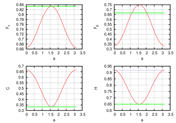
Figure 2: (color online) Quantities of the equatorial cloner as a function of the angle $\theta$ on the Bloch sphere. $F_{c}$ is the cloning fidelity, $F_{p}$ is the process fidelity, $C$ is the concurrence of the clones, $H$ is the von Neumann entropy. In all the figures, the respective quantity of the UCQC is also plotted, these are the straight lines, the curves represent the quantity for the equatorial cloner. In case of the entropy the entropy of the clone is always equal to the entropy of the bipartite states of the two clones. The lower straight line is the entropy of the clone, while the upper is the entropy of the bipartite state for the UCQC.

We have also carried out the same analysis with the completely mixed ancilla as for the case of the universal cloner. As reflected by the last four lines of Table 1, the conclusion to be drawn is the same as for the universal case: the cloner for pure ancilla becomes a classical copier for a completely mixed ancilla. It is possible to design a cloner for the completely mixture, which works for the pure ancilla as well.

Again it is interesting though to take a look at the Choi matrices of the above cloners, given in Eqs. (26) and (27). It appears that the spectrum of these matrices is the same as that of the universal cloners.

Another question to be addressed in the case of a phase-covariant cloner is that of the dependence on the ancilla. To investigate this we have considered a case when the target set is the equator rotated by a given angle about the $x$ axis. Carrying out this analysis for various angles, we have found that the resulting cloner has the very parameters of the above-detailed equatorial cloner: the designed cloner is optimal and anisotropic, independently of the angle between the ancilla state and the chosen main circle. This is illustrated in terms of cloning fidelity in Fig. 3, for a main circle rotated by $\pi/4$. This is not very surprising for symmetry reasons, nevertheless it again demonstrates the power of the applied numerical technique.

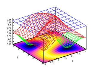
Figure 3: (color online) The cloning fidelity as a function of the spherical coordinates on the Bloch sphere of the input states, for a cloner designed for cloning the equator of the Bloch sphere rotated by $\pi/4$ about the $x$ axis. The upper flat plane represents $5/6$, the fidelity of the optimal cloner. The plotted quantity is dimensionless.

IV Conclusions and outlook

We have explicitly designed universal and phase covariant process optimized quantum cloners: quantum cloners that are optimized for the fidelity of the state of the whole set of output states to that of a product of ideal clones. We studied their design for $1\to 2$ qubit cloners numerically, via semidefinite programming. In all the studied cases the so-designed cloners have been found to be optimal cloners with respect to the fidelity of clones to the originals, too.

For the phase covariant case we have found the result to be expected according to Ref. DAriano . We have analyzed the operation of this cloner on the whole Bloch sphere as well, with respect to state purity and entanglement.

Our result demonstrates the power of the method introduced in Ref. koenraad in designing particular quantum circuits for different purposes in a neat and automated numerical way. The only requirement for the process to be approximated is that its ideal output should be pure states and one has to be able to average over the possible input states.

Appendix A Choi matrices of some cloners

In what follows we write rational numbers as matrix elements. The results of our calculations were their floating point counterparts within numerical precision, so we use the rational counterparts for sake of clarity. It would be possible to verify analytically that these are the optima indeed, by calculating the the duality gap in the optimization.

Universal cloner with pure ancilla

The nonzero elements of the Choi matrix are:

$$X=\setcounter{MaxMatrixCols}{16}\begin{pmatrix}\frac{2}{3}&0&0&0&0&0&0&0&0&\frac{1}{3}&\frac{1}{3}&0&0&0&0&0\\ 0&\frac{1}{6}&\frac{1}{6}&0&0&0&0&0&0&0&0&\frac{1}{3}&0&0&0&0\\ 0&\frac{1}{6}&\frac{1}{6}&0&0&0&0&0&0&0&0&\frac{1}{3}&0&0&0&0\\ 0&0&0&0&0&0&0&0&0&0&0&0&0&0&0&0\\ 0&0&0&0&\frac{1}{4}&0&0&0&0&0&0&0&0&0&0&0\\ 0&0&0&0&0&\frac{1}{4}&0&0&0&0&0&0&0&0&0&0\\ 0&0&0&0&0&0&\frac{1}{4}&0&0&0&0&0&0&0&0&0\\ 0&0&0&0&0&0&0&\frac{1}{4}&0&0&0&0&0&0&0&0\\ 0&0&0&0&0&0&0&0&0&0&0&0&0&0&0&0\\ \frac{1}{3}&0&0&0&0&0&0&0&0&\frac{1}{6}&\frac{1}{6}&0&0&0&0&0\\ \frac{1}{3}&0&0&0&0&0&0&0&0&\frac{1}{6}&\frac{1}{6}&0&0&0&0&0\\ 0&\frac{1}{3}&\frac{1}{3}&0&0&0&0&0&0&0&0&\frac{2}{3}&0&0&0&0\\ 0&0&0&0&0&0&0&0&0&0&0&0&\frac{1}{4}&0&0&0\\ 0&0&0&0&0&0&0&0&0&0&0&0&0&\frac{1}{4}&0&0\\ 0&0&0&0&0&0&0&0&0&0&0&0&0&0&\frac{1}{4}&0\\ 0&0&0&0&0&0&0&0&0&0&0&0&0&0&0&\frac{1}{4}\end{pmatrix}$$ (24)

The rank of this matrix is 10. Its eigenvalues are $1.0$ (multiplicity $2$) and $0.25$ (multiplicity $8$)

Universal cloner with completely mixed ancilla

The Choi matrix reads:

$$X=\setcounter{MaxMatrixCols}{16}\begin{pmatrix}\frac{2}{3}&0&0&0&0&0&0&0&0&\frac{1}{3}&\frac{1}{3}&0&0&0&0&0\\ 0&\frac{1}{6}&\frac{1}{6}&0&0&0&0&0&0&0&0&\frac{1}{3}&0&0&0&0\\ 0&\frac{1}{6}&\frac{1}{6}&0&0&0&0&0&0&0&0&\frac{1}{3}&0&0&0&0\\ 0&0&0&0&0&0&0&0&0&0&0&0&0&0&0&0\\ 0&0&0&0&\frac{2}{3}&0&0&0&0&0&0&0&0&\frac{1}{3}&\frac{1}{3}&0\\ 0&0&0&0&0&\frac{1}{6}&\frac{1}{6}&0&0&0&0&0&0&0&0&\frac{1}{3}\\ 0&0&0&0&0&\frac{1}{6}&\frac{1}{6}&0&0&0&0&0&0&0&0&\frac{1}{3}\\ 0&0&0&0&0&0&0&0&0&0&0&0&0&0&0&0\\ 0&0&0&0&0&0&0&0&0&0&0&0&0&0&0&0\\ \frac{1}{3}&0&0&0&0&0&0&0&0&\frac{1}{6}&\frac{1}{6}&0&0&0&0&0\\ \frac{1}{3}&0&0&0&0&0&0&0&0&\frac{1}{6}&\frac{1}{6}&0&0&0&0&0\\ 0&\frac{1}{3}&\frac{1}{3}&0&0&0&0&0&0&0&0&\frac{2}{3}&0&0&0&0\\ 0&0&0&0&0&0&0&0&0&0&0&0&0&0&0&0\\ 0&0&0&0&\frac{1}{3}&0&0&0&0&0&0&0&0&\frac{1}{6}&\frac{1}{6}&0\\ 0&0&0&0&\frac{1}{3}&0&0&0&0&0&0&0&0&\frac{1}{6}&\frac{1}{6}&0\\ 0&0&0&0&0&\frac{1}{3}&\frac{1}{3}&0&0&0&0&0&0&0&0&\frac{2}{3}\end{pmatrix}$$ (25)

The rank of this matrix is $4$, the only eigenvalue is $1.0$.

Equator, pure ancilla

The Choi matrix reads:

$$X=\setcounter{MaxMatrixCols}{16}\begin{pmatrix}\frac{1}{3}&0&0&0&0&0&0&0&0&\frac{1}{3}&\frac{1}{3}&0&0&0&0&0\\ 0&\frac{1}{3}&\frac{1}{3}&0&0&0&0&0&0&0&0&\frac{1}{3}&0&0&0&0\\ 0&\frac{1}{3}&\frac{1}{3}&0&0&0&0&0&0&0&0&\frac{1}{3}&0&0&0&0\\ 0&0&0&0&0&0&0&0&0&0&0&0&0&0&0&0\\ 0&0&0&0&\frac{1}{4}&0&0&0&0&0&0&0&0&0&0&0\\ 0&0&0&0&0&\frac{1}{4}&0&0&0&0&0&0&0&0&0&0\\ 0&0&0&0&0&0&\frac{1}{4}&0&0&0&0&0&0&0&0&0\\ 0&0&0&0&0&0&0&\frac{1}{4}&0&0&0&0&0&0&0&0\\ 0&0&0&0&0&0&0&0&0&0&0&0&0&0&0&0\\ \frac{1}{3}&0&0&0&0&0&0&0&0&\frac{1}{3}&\frac{1}{3}&0&0&0&0&0\\ \frac{1}{3}&0&0&0&0&0&0&0&0&\frac{1}{3}&\frac{1}{3}&0&0&0&0&0\\ 0&\frac{1}{3}&\frac{1}{3}&0&0&0&0&0&0&0&0&\frac{1}{3}&0&0&0&0\\ 0&0&0&0&0&0&0&0&0&0&0&0&\frac{1}{4}&0&0&0\\ 0&0&0&0&0&0&0&0&0&0&0&0&0&\frac{1}{4}&0&0\\ 0&0&0&0&0&0&0&0&0&0&0&0&0&0&\frac{1}{4}&0\\ 0&0&0&0&0&0&0&0&0&0&0&0&0&0&0&\frac{1}{4}\end{pmatrix}$$ (26)

Its rank is $10$, with the same eigenvalues and multiplicities as the matrix for the universal cloner with pure ancilla.

Equator, completely mixed ancilla

The Choi matrix reads:

$$X=\setcounter{MaxMatrixCols}{16}\begin{pmatrix}\frac{1}{3}&0&0&0&0&0&0&0&0&\frac{1}{3}&\frac{1}{3}&0&0&0&0&0\\ 0&\frac{1}{3}&\frac{1}{3}&0&0&0&0&0&0&0&0&\frac{1}{3}&0&0&0&0\\ 0&\frac{1}{3}&\frac{1}{3}&0&0&0&0&0&0&0&0&\frac{1}{3}&0&0&0&0\\ 0&0&0&0&0&0&0&0&0&0&0&0&0&0&0&0\\ 0&0&0&0&\frac{1}{3}&0&0&0&0&0&0&0&0&\frac{1}{3}&\frac{1}{3}&0\\ 0&0&0&0&0&\frac{1}{3}&\frac{1}{3}&0&0&0&0&0&0&0&0&\frac{1}{3}\\ 0&0&0&0&0&\frac{1}{3}&\frac{1}{3}&0&0&0&0&0&0&0&0&\frac{1}{3}\\ 0&0&0&0&0&0&0&0&0&0&0&0&0&0&0&0\\ 0&0&0&0&0&0&0&0&0&0&0&0&0&0&0&0\\ \frac{1}{3}&0&0&0&0&0&0&0&0&\frac{1}{3}&\frac{1}{3}&0&0&0&0&0\\ \frac{1}{3}&0&0&0&0&0&0&0&0&\frac{1}{3}&\frac{1}{3}&0&0&0&0&0\\ 0&\frac{1}{3}&\frac{1}{3}&0&0&0&0&0&0&0&0&\frac{1}{3}&0&0&0&0\\ 0&0&0&0&0&0&0&0&0&0&0&0&0&0&0&0\\ 0&0&0&0&\frac{1}{3}&0&0&0&0&0&0&0&0&\frac{1}{3}&\frac{1}{3}&0\\ 0&0&0&0&\frac{1}{3}&0&0&0&0&0&0&0&0&\frac{1}{3}&\frac{1}{3}&0\\ 0&0&0&0&0&\frac{1}{3}&\frac{1}{3}&0&0&0&0&0&0&0&0&\frac{1}{3}\end{pmatrix}$$ (27)

Its rank is $4$, with the same eigenvalue and multiplicities as the universal cloner with completely mixed ancilla.