Numerical calculation of magnetic form factors of complex shape nano-particles coupled with micromagnetic simulations.

Abstract

We investigate the calculation of the magnetic form factors of nano-objects with complex geometrical shapes and non homogeneous magnetization distributions. We describe a numerical procedure which allows to calculate the 3D magnetic form factor of nano-objects from realistic magnetization distributions obtained by micromagnetic calculations. This is illustrated in the canonical cases of spheres, rods and platelets. This work is a first step towards a 3D vectorial reconstruction of the magnetization at the nanometric scale using neutron scattering techniques.

I Introduction

The recent progress in solid state chemistry has led to the possibility of synthesizing nano-objects of non spherical shapes: wires by organometallic chemistry soulantica2009 or electrochemistry wade2005 . In particular, the use of the polyol process has made it possible to produce well defined monodisperse magnetic nano-objects. Depending on the synthesis conditions, various shapes of particles can be obtained such as rods, wires, dumbbells, diabolos, platelets… (see Figure 1) viau2008 ; soumare2008 ; soumare2009 . These are the typical forms of magnetic nano-objects which will be the focus of this communication. While magnetic nanospheres (as found for example in ferrofluids) have been extensively studied by Small Angle Neutron Scattering michels_rev ; Wiedenmann2003 ; Wiedenmann2004 ; wiedenmann2006 ; michels2005 ; michels2006 , more complex shaped magnetic nano-objects have rarely been studied.

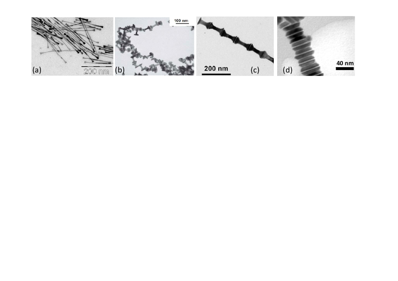
Figure 1: TEM images of magnetic nano-objects synthesized in various conditions: (a) $Co_{80}Ni_{20}$ nanowires with rounded tips of length $200$ nm and diameter $7$ nm ; (d) $Co_{50}Ni_{50}$ dumbbells ; (e) $Co$ diabolos and (f) $Co$ platelets.

In this communication we focus on the detailed description and calculation of neutron scattering on magnetic nano-objects in SANS experiments. We describe numerical tools to calculate the magnetic form factors of arbitrary shape nano-objects. We present a practical procedure which allows to calculate magnetic form factors either from an a priori knowledge of the magnetization distribution or from a minimization of the micro-magnetic configuration.

II Nuclear and magnetic form factors calculations for neutrons

In this section we first recall the interaction of neutrons with small nano-objects. We introduce the nuclear and magnetic form factors of nano-objects and describe the quantities which can be measured in a Polarized Small Angle Neutron Scattering (PSANS) experiment. A practical way of calculating the magnetic form factor of complex nano-objects is then presented.

II.1 Nuclear and magnetic form factors

Let us consider a magnetic nano-object of nuclear Scattering Length Density (SLD) $\rho\left(\vec{r}\right)$ which creates an induction distribution $\overrightarrow{B}\left(\vec{r}\right)$. We define the nuclear form factor $f_{N}(\vec{Q})$ as the Fourier transform of the nuclear SLD distribution, $\vec{Q}=\vec{k_{f}}-\vec{k_{i}}$ being the scattering wave-vector:

$$f_{N}\left(\vec{Q}\right)\propto\iiint\rho\left(\vec{r}\right)e^{-i\vec{Q}.\vec{r}}d\vec{r}$$ (1)

Similarly we define the magnetic form factor $\vec{f}_{B}\left(\vec{Q}\right)$ as the Fourier transform of the induction field $\overrightarrow{B}\left(\vec{r}\right)$:

$$\vec{f}_{B}\left(\vec{Q}\right)\propto\iiint\vec{B}\left(\vec{r}\right)e^{-i\vec{Q}.\vec{r}}d\vec{r}$$ (2)

It can be shown that only the component of $\vec{f}_{B}\left(\vec{Q}\right)$ perpendicular to $\vec{Q}$ contributes to the scattering bruckel2009 :

$$\vec{f}_{B\bot}=\vec{q}\times\vec{f}_{B}\times\vec{q}=\vec{f}_{B}-\left(\vec{f}_{B}\cdot\vec{q}\right)\vec{q}$$ (3)

with $\vec{q}=\frac{\vec{Q}}{|Q|}$ being the unit vector along the $\vec{Q}$ direction.

The total scattering cross section writes:

$$\frac{d\sigma}{d\Omega}\propto\left|f_{N}\left(\vec{Q}\right)+\vec{f}_{B\bot}\left(\vec{Q}\right)\cdot\vec{\sigma}\right|^{2}$$ (4)

where we recall that $\vec{\sigma}$ is the neutron spin operator.

In the case of polarized neutrons with polarization analysis, it is possible to measure 4 quantities corresponding to “Non Spin Flip” (NSF, (++) or (- -)) and “Spin Flip” (SF, (+-) or (-+)) scattering as recently experimentally put into evidence honecker ; Krycka2010 :

$$\begin{array}[]{l}\begin{array}[]{c}\frac{d\sigma^{++}}{d\Omega}=\left|f_{N}(\vec{Q})+f_{B_{\bot z^{\prime}}}(\vec{Q})\right|^{2}\\ \frac{d\sigma^{--}}{d\Omega}=\left|f_{N}(\vec{Q})-f_{B_{\bot z^{\prime}}}(\vec{Q})\right|^{2}\\ \frac{d\sigma^{+-}}{d\Omega}=\left|f_{B_{\bot x^{\prime}}}(\vec{Q})-i\>f_{B_{\bot y^{\prime}}}(\vec{Q})\right|^{2}\\ \frac{d\sigma^{-+}}{d\Omega}=\left|f_{B_{\bot x^{\prime}}}(\vec{Q})+i\>f_{B_{\bot y^{\prime}}}(\vec{Q})\right|^{2}\end{array}\end{array}$$ (5)

where $f_{B_{\bot x^{\prime}}}(\vec{Q})$, $f_{B_{\bot y^{\prime}}}(\vec{Q})$ and $f_{B_{\bot z^{\prime}}}(\vec{Q})$ refer to the component of $\vec{f}_{B_{\bot}}\left(\vec{Q}\right)$ along the $(Ox^{\prime})$, $(Oy^{\prime})$ and $(Oz^{\prime})$ axis respectively, where $(Oz^{\prime})$ is the quantification axis of the neutron spin defined by the applied magnetic field. If the induction distribution is even around the $(Ox^{\prime})$ and $(Oy^{\prime})$ axes, the Fourier transforms $f_{B_{\bot x^{\prime}}}(\vec{Q})$ and $f_{B_{\bot y^{\prime}}}(\vec{Q})$ are real so that the two spin-flip cross sections are equal. These formulae are derived from Eq. 4 using the Pauli matrices Pauli .

In the case of polarized neutrons without polarization analysis which in practice is the situation encountered in most PSANS experiments, the two scattering intensities which can be measured are: until now, 2 quantities can be measured:

$$\begin{array}[]{l}\frac{d\sigma^{+}}{d\Omega}=\frac{d\sigma^{++}}{d\Omega}+\frac{d\sigma^{+-}}{d\Omega}=\\ \left|f_{N}(\vec{Q})+f_{B_{\bot z^{\prime}}}(\vec{Q})\right|^{2}+\left|f_{B_{\bot x^{\prime}}}(\vec{Q})+i\>f_{B_{\bot y^{\prime}}}(\vec{Q})\right|^{2}\\ \\ \frac{d\sigma^{-}}{d\Omega}=\frac{d\sigma^{--}}{d\Omega}+\frac{d\sigma^{-+}}{d\Omega}=\\ \left|f_{N}(\vec{Q})-f_{B_{\bot z^{\prime}}}(\vec{Q})\right|^{2}+\left|f_{B_{\bot x^{\prime}}}(\vec{Q})-i\>f_{B_{\bot y^{\prime}}}(\vec{Q})\right|^{2}\end{array}$$ (6)

For non polarized neutron scattering:

$$\begin{array}[]{l}\frac{d\sigma}{d\Omega}=\frac{d\sigma^{+}}{d\Omega}+\frac{d\sigma^{-}}{d\Omega}=\left|f_{N}\left(\vec{Q}\right)\right|^{2}+\left|\vec{f}_{B\bot}(\vec{Q})\right|^{2}\end{array}$$ (7)

II.2 Practical calculation of the nuclear and magnetic form factors

We shall now discuss how to calculate in practice the quantity $\vec{f}_{B\bot}(\vec{Q})$. A first approach consists in assuming an a priori knowledge of the magnetization distribution in the particle (for example, $\vec{M}$ can be assumed to be homogeneous). Under this assumption, the induction field distribution $\overrightarrow{B}\left(\vec{r}\right)$ can be calculated using standard electromagnetic softwares. In the case of objects with an axis of revolution, we suggest the use of the Femm package FEMM . The package provides various tools (scripting langage LUA, Octavefemm interface to Octave or Matlab, Mathfemm interface to Mathematica) which allows extracting the induction field distribution $\overrightarrow{B}\left(\vec{r}\right)$ from the electromagnetic calculation.

A more general approach, with no assumptions on the magnetization distribution in the nanoparticle calculates the magnetization distribution in the particle under a given applied magnetic field. Several micromagnetic packages have become available for non expert users during the last few years (OOMMF oommf , MagPar magpar , Nmag nmag ). We have used the Nmag package since it is based on finite elements and is thus especially well suited to the types of particles encountered in SANS scattering (spheres, cylinders, disks). The procedure consists in defining an object geometry and discretization using the Netgen mesher netgen (Figure 3). The 3D magnetic moments distribution $\overrightarrow{M}\left(\vec{r}\right)$ in the object can then be calculated using the Nmag package (Figure 3e).

In order to perform a numerical calculation of the magnetic form factors of such magnetic objects, a volume of space $V$ containing the objects is defined. Its dimensions $L_{x}\times L_{y}\times L_{z}$ are such that this volume is significantly large than the nanoobjects (3-10 times). From the magnetization distribution $\overrightarrow{M}(\vec{r})$ in the nano-object, the induction field $\overrightarrow{B}\left(\vec{r}\right)$ can be calculated in the whole volume $V$. In practice, this induction field $\overrightarrow{B}\left(\vec{r}\right)$ is calculated on a regular grid and mapped on a 3D matrix of size $(n_{x},n_{y},n_{z})$. Python scripts performing this task are available on the LLB Website Scripts . This induction distribution is then exported into octave or matlab in order to perform numerical calculations of the magnetic form factor $\vec{f}_{B}(\vec{Q})$ using equations (2) and (3). The corresponding scripts are freely available at Scripts . One obtains a set of three 3D matrices $\left\{f_{Bx}(\vec{Q}),\,f_{By}(\vec{Q}),\,f_{Bz}(\vec{Q})\right\}$ describing the 3 components of the magnetic form factor in the reciprocal space. The reciprocal space is mapped with a sampling given by $\Delta Q=\frac{2\pi}{L_{i}}$ and the useful accessible $Q$-range goes from $Q_{min}=\frac{2\pi}{L_{i}}$ to about $Q_{i}^{max}\sim 0.5\times\frac{2\pi}{L_{i}}n_{i}$ (e.g. for $L_{i}=100nm$ and $n_{i}=100$, $0.06<Q<3nm^{-1}$ )

The Fourier transforms of the induction field are performed using a FFT algorithm with the condition that the dimensions $(n_{x},n_{y},n_{z})$ of the matrices are powers of 2. Since we are dealing with 3D matrices, the memory requirements diverge rather quickly as the matrices sizes increase. A matrix size of $128\times 128\times 128$ provides both a reasonable memory footprint (32 MBytes / matrix) and fast calculations times ($50ms$ per FFT on a standard desktop computer). Such a sampling rate provides accurate Fourier transforms in the reciprocal space over 2 orders of magnitude (see Figure 5 for example). We found that a volume of space $V$ about 6 times larger (i.e. $L_{x}=6D$ for a sphere of diameter $D$) than the studied object provided good results in the $Q$ range of interest.

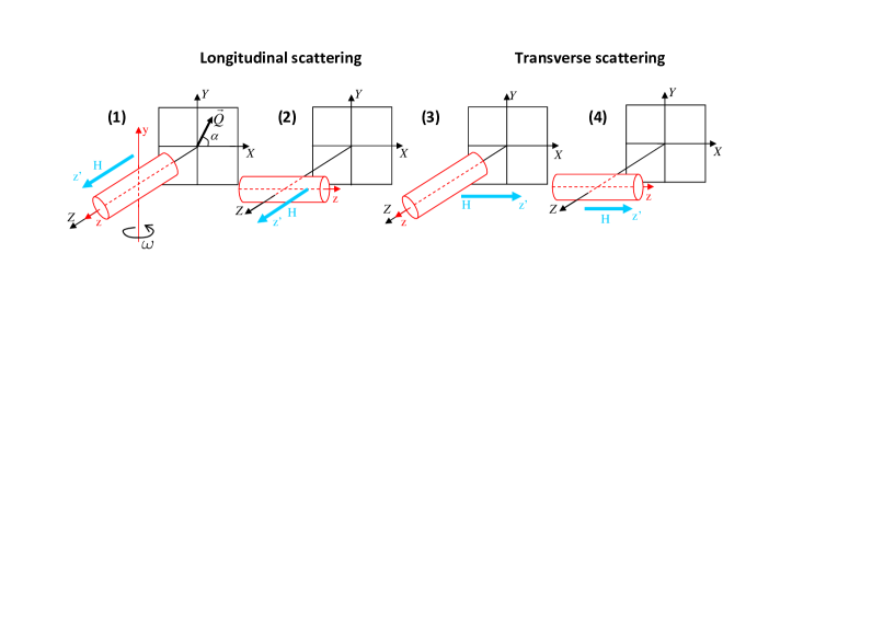
Figure 2: The different scattering that will be considered. The neutron beam is incident along the $(OZ)$ direction. $(XY)$ defines the scattering plane. The longitudinal (1-2) and transverse (3-4) scattering geometries correspond to a magnetic field applied along $(OZ)$ and $(OX)$ respectively. The scattering object can be oriented with its easy axis parallel (1-4) or perpendicular (2-3) to the applied field.

We now define the scattering geometries that will be considered in the actual numerical calculations presented in the next section. We first underline that in the general case of polarized neutron scattering on anisotropic particles, it is necessary to define 3 axis systems. The first one $(x,y,z)$ is attached to the studied nano-objects. The second one $(X,Y,Z)$ describes the spectrometer geometry. The third one $(x^{\prime},y^{\prime},z^{\prime})$ describes the orientation of the quantification axis (defined by the applied magnetic field along $z^{\prime}$). In order to describe a scattering experiment, it is necessary to define the relative orientations of these 3 sets of axis.

In order to simplify the presentation and to comply with experimental conditions, we consider a scattering plane $\left(Q_{X}=Q\cos\alpha,\>Q_{Y}=Q\sin\alpha\right)$ corresponding to the 2D detector plane of a SANS spectrometer $(XOY)$. For each scattering direction $\alpha$ in the scattering plane, the perpendicular components of the magnetic form factor $\vec{f}_{\bot}\left(\theta,r\right)$ can be calculated using equation (3):

$$\left(\begin{array}[]{c}f_{B_{\perp X}}\\ f_{B_{\perp Y}}\\ f_{B_{\perp Z}}\end{array}\right)=\left(\begin{array}[]{c}f_{B_{X}}-(f_{B_{X}}\cos\alpha+f_{B_{Y}}\sin\alpha)\cos\alpha\\ f_{B_{Y}}-(f_{B_{X}}\cos\alpha+f_{B_{Y}}\sin\alpha)\sin\alpha\\ f_{B_{Z}}\end{array}\right)$$ (8)

Note that the above formula is only valid in the $(Q_{X},\>Q_{Y})$ scattering plane. In the practical procedure, the magnetic induction distribution is calculated in the $(xyz)$ reference frame where $(Oz)$ is the revolution axis of the object. The examples proposed in Scripts follow this convention. We define $\omega$ as the rotation angle of the object around the $(OY)$ axis. With these conventions, for $\omega=0$, a cylinder is aligned along the $(OZ)$ axis. For $\omega=90\text{\textdegree}$, a cylinder is aligned along the $(OX)$ axis. The distribution $\overrightarrow{B}\left(\vec{r}\right)_{XYZ}$ in the spectrometer axis is obtained by a rotation $\omega$ :

$$\left(\begin{array}[]{c}B_{\perp X}\\ B_{\perp Y}\\ B_{\perp Z}\end{array}\right)=\left(\begin{array}[]{ccc}cos\omega&0&sin\omega\\ 0&1&0\\ -sin\omega&0&cos\omega\end{array}\right)\left(\begin{array}[]{c}B_{\perp x}\\ B_{\perp x}\\ B_{\perp z}\end{array}\right)$$ (9)

For the sake of illustration, we shall not include both the nuclear scattering and the magnetic scattering in the calculations. Even though this is not realistic in a general scattering experiment where the nuclear contribution is usually large, such situations can be encountered in SANS experiments: the nuclear contrast of cobalt particles can easily be matched by using an appropriate deuterated solvent Wiedenmann2003 ; Wiedenmann2004 ; ferromagnetic particles in a paramagnetic matrix also allow to extinguish the nuclear contrast michels2006 . Ignoring the nuclear scattering effects will allow us to focus on the magnetic effects which are the scope of this communication.

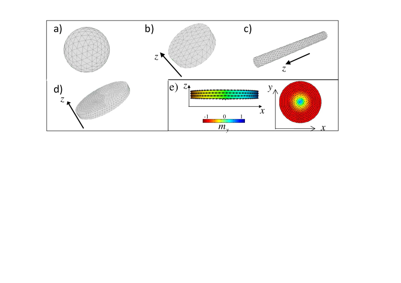
Figure 3: Typical meshes obtained from the Netgen mesher for the different nano-objects: (a) a sphere of diameter $D=10$ nm, (b) a flat disk of diameter $D=20$ nm and height $h=2.5$ nm, (c) a cylinder of diameter $D=10$ nm and length $L=50$ nm, (d) a disk of diameter $D=50$ nm and height $h=5$ nm. Note that the distance between two nodes is around 1 nm. (e) Maps of the magnetic moments distribution at remanence for the disk defined in (d). The colors encode the $y$-component of the magnetization ($m_{y}=M_{y}/M$) in the profile view (left) and $z$-component of the magnetization ($m_{z}=M_{z}/M$) viewed from the top (right).

In the following, we shall different relative orientations of the applied magnetic field direction with respect to the scattering plane:

1. Longitudinal scattering $(H\parallel OZ)$ . Equation (5) becomes:

   $$\begin{array}[]{l}\frac{d\sigma^{++}}{d\Omega}=\frac{d\sigma^{--}}{d\Omega}=\left|f_{B_{\bot Z}}(\vec{Q})\right|^{2}\\ \frac{d\sigma^{+-}}{d\Omega}=\frac{d\sigma^{-+}}{d\Omega}=\left|f_{B_{\bot X}}(\vec{Q})\mp i\>f_{B_{\bot Y}}(\vec{Q})\right|^{2}\end{array}$$ (10)

2. Transverse scattering $(H\parallel OX)$ . Equation (5) becomes:

   $$\begin{array}[]{l}\frac{d\sigma^{++}}{d\Omega}=\frac{d\sigma^{--}}{d\Omega}=\left|f_{B_{\bot X}}(\vec{Q})\right|^{2}\\ \frac{d\sigma^{+-}}{d\Omega}=\frac{d\sigma^{-+}}{d\Omega}=\left|f_{B_{\bot Y}}(\vec{Q})\mp i\>f_{B_{\bot Z}}(\vec{Q})\right|^{2}\end{array}$$ (11)

Note that even though the above formulae are very similar, the key parameter is the distribution $f_{B_{\bot}}(\vec{Q})$ with respect to the scattering plane. The scattering geometries (1)-(4) presented on Figure 2 will lead to qualitatively different results which are discussed in the next section.

III Model calculations

In this section we will present the calculation of the magnetic form factors of different types of nano-objects: (a) a sphere of diameter $D=10$ nm, (b) a flat disk of diameter $D=10$ nm and height $h=2.5$ nm and (c) a cylinder of diameter $D=10$ nm and length $L=50$ nm. These objects are presented in Figure 3. The magnetic parameters used are the following: magnetization saturation of cobalt $M=1.4\times 10^{6}$ A.m^-1($\equiv$1.76 T); exchange stiffness $A=1.2\times 10^{11}$ J.m^-1. Moreover, a uniaxial magnetocrystalline anisotropy $K=7\times 10^{5}$ J.m^-3 along $z$ was considered in the case of the flat disk (Figure 3b) in order to force the magnetic moments to be normal to the disk surface. In a first step, the remanent configuration was determined for all the objects. It reveals a rather homogeneous distribution of the magnetic moments along the $Oz$ direction for objects (a), (b) and (c). This is due to the fact that these objects are to the first order approximations of elliptical objects in which the demagnetizing field in homogeneous. For simplicity, only nano-objects with a quasi uniform magnetic moments distribution have been considered. However, more complex distributions can be considered as it is highlight for a disk of diameter $D=50$ nm and height $h=5$ nm within which a vortex state appears (see Figure 3e).

We perform numerical calculation of the 3D nuclear form factors so as to be able to compare the results with analytical formulae and validate the numerical procedure. As a next step, we perform calculations of the magnetic form factors where we illustrate the contributions of the demagnetizing and the dipolar fields.

III.1 Validation of the numerical procedure: application to the calculation of nuclear form factors

Although this paper is devoted to the magnetic form factors of nano-objects, we have also numerically calculated the 3D nuclear form factor of these objects in order to check the applicability of our numerical algorithm. When calculating the 3D nuclear form factor, the volume of space $V$ containing the object is mapped onto a 3D matrix $G_{x,y,z}$ describing the object geometry in such a way that $G_{x,y,z}=1$ for $(x,y,z)$ inside the object and $G_{x,y,z}=0$ for $(x,y,z)$ outside the object.

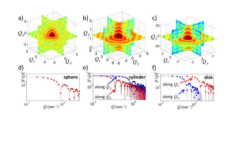
Figure 4: Numerically calculated form factors (circles) and comparison with analytical formulas (continuous lines). a), b) and c) correspond to 3D form factors calculated for the sphere $D=10$, the cylinder ($D=10$ nm, $L=50$ nm), the flat disk ($D=10$ nm, $h=2.5$ nm) and 1D cuts of the form factor in the reciprocal space in specific directions.

Figures 4a-b-c present the 3D nuclear form factors calculated for the sphere ($D=10$ nm), the flat disk ($D=10$ nm, $h=2.5$nm) and the cylinder ($D=10$ nm, $L=50$ nm) defined in Figure 3. The scattering is isotropic in the sphere case and anisotropic in the other cases. The nuclear form factors of these simple objects are well known and can be analytically calculated glatter . We can thus compare our numerical results with the analytical formulae. Figures 4d-e-f compare the numerical and analytical calculations along the main directions in the reciprocal space (in nm^-1) for the different objects. The agreement is satisfactory for all the objects which proves the applicability of our numerical calculations.

These results show that it is possible to calculate rather accurately, in a single shot, the form factor in a $Q$-range extending over 2 decades with scattering intensities extending over 3 decades. If one would be interested in a different $Q$-range, it is necessary to resize the $V$ box around the object. As $Q_{min}=\frac{2\pi}{L_{i}}$, in order to probe smaller Q values, the size $L_{i}$ of the box should be increased As $Q_{i}^{max}\sim 0.5\times\frac{2\pi}{L_{i}}n_{i}$, in order to probe larger Q values, either the size $L_{i}$ of the box should be decreased of the number of mapping points $n_{i}$ should be increased. This is similar to a real SANS experiment where the measuring conditions are changed in order to cover a wider $Q$-range.

In the following we shall however restrict ourselves to a $V$ box $6\times 6\times 6$ times the size of the object, which provides an appropriate sampling in the $Q$ space for our demonstrations.

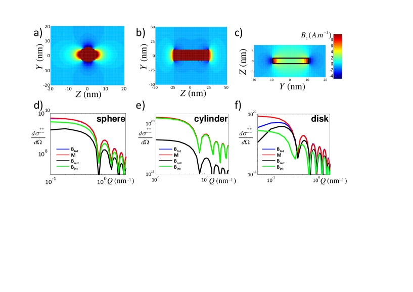
Figure 5: Longitudinal scattering on 3 types of objects (sphere, cylinder and disk) magnetized along the applied field. a), b), and c) Induction distribution in ($YZ$) plane for a sphere, a cylinder and a disk magnetized along the $Z$ direction. d), e) and f) Scattering cross sections of different magnetic contributions: the magnetization only ($\vec{M}(\vec{r)}$), the internal magnetic induction ($\vec{B}_{int.}(\vec{r)}$), the dipolar field created by the magnetic moments outside the object ($\vec{B}_{ext.}(\vec{r)}$) and the whole magnetic induction ($\vec{B}{}_{tot.}(\vec{r)}=\vec{B}_{int.}(\vec{r)}+\vec{B}_{ext.}(\vec{r)}$).

III.2 Case of magnetic objects

The same calculation procedure was applied to the case of magnetic objects. Figure 5 presents the calculation of the magnetic form factors in the case of the 3 canonical geometries (sphere, disk and cylinder). A first reference calculation was performed by calculating the form factor of an homogeneously magnetized sample and for which only the magnetization inside the sample was considered (blue lines on Figure 5). A second calculation was performed where the form factor of the induction map was also included. The induction map is plotted on Figure 5 a-c. We considered the induction in the sample given by $\vec{B}_{int.}(\vec{r)}=\mu_{0}\left(\vec{M}(\vec{r)}+\vec{H}_{d}(\vec{r)}\right)$ where $\vec{H}_{d}(\vec{r)}$ is the demagnetizing fields and the stray fields outside the sample ($\vec{B}_{ext.}(\vec{r)}$). The contribution of these inductions distributions was calculated separately (black and green curves). The sum of these contributions $\vec{B}_{tot.}(\vec{r)}$ overlaps with the form factor simply obtained from the magnetization distribution (see figure 5d-e-f). The deviation observed at low $Q$ are numerical artifacts due to the fact that the stray fields expand beyond the calculation box. This numerically demonstrates that the magnetic form factor can be obtained by considering the magnetization distribution without taking into account the demagnetization fields and the stray fields outside the sample.

IV Conclusion

We have developed numerical tools Scripts which permits the calculations of the structural and magnetic form factor of nano-objects with complex geometrical shapes. Such calculations were until recently limited due to the extensive memory usage of 3 dimensional FFT calculations. As Polarized SANS spectrometers are becoming widely available the problem of quantitatively processing the data obtained on complex magnetic nano-systems will arise. This first step will allow experimentalists to compare their measurements with realistic models of the magnetization in their nano-systems. In the future, with the widespread availability of systems with tens of gigabytes of memory, one may consider applying similar methods for the numerical calculation of complex structure factors.

- (1) T. L. Wade, J. E. Wegrowe, European Physical Journal - Applied Physics, 29, 3 (2005)
- (2) K. Soulantica, F. Wetz, J. Maynadie et al., Appl. Phys. Lett. 95, 152504 (2009).
- (3) G. Viau, C. Garcia, T. Maurer et al. Phys. Stat. Sol. A - Applications and Materials Science 206 663-666 (2009).
- (4) Y. Soumare, J. -Y. Piquemal, T. Maurer et al. J. of Materials Chemistry 18, 5696-5702 (2008).
- (5) Y. Soumare, C. Garcia, T. Maurer et al., Advanced Functional Materials 19, 1971 (2009)
- (6) A. Michels and J. Weissmï¿œller, Rep. Prog. Phys., 71 066501 (2008)
- (7) A. Hoell, M. Kammel, A. Heinemann and A. Wiedenmann, J. Appl. Cryst. 36, 558 (2003)
- (8) K. Butter, A. Hoell, A. Wiedenmann, A. V. Petukhov and G.-J. Vroege, J. Appl. Cryst. 37, 847 (2004)
- (9) A. Wiedenmann , M. Kammel , A. Heinemann and U. Keiderling, Journal of Physics: Condensed Matter 18, S2713 (2006)
- (10) A. Michels, C. Vecchini, O. Moze, K. Suzuki, J. M. Cadogan, P. K. Pranzas and J. Weissmœller, Europhys. Lett., 72 (2), 249 (2005)
- (11) A. Michels, C. Vecchini and O. Moze, K. Suzuki, P. K. Pranzas, J. Kohlbrecher, J. Weissmœller, Physical Review B, 74, 134407 (2006)
- (12) T. Bruckel, G. Heger, D. Richter and R. Zorn, Neutron Scattering - Lectures of the Laboratory Course held at the FZ Jœlich, Vol. 28 (2009) p. 3-22. ISSN 1433-5506 ISBN 3-89336-395-5. http://hdl.handle.net/2128/418
- (13) D. Honecker, A. Ferdinand, F. Dobrich, C. D. Dewhurst, A. Wiedenmann, C. Gomez-Polo, K. Suzuki and A. Michels, Eur. Phys. J. B (2010), DOI: 10.1140/epjb/e2010-00191-5
- (14) K. L. Krycka, R. A. Booth, C. R. Hogg, Y. Ijiri, J. A. Borchers, W. C. Chen, S. M.Watson, M. Laver, T. R. Gentile, L. R. Dedon, S. Harris, J. J. Rhyne and S. A. Majetich, Phys. Rev. Lett., 104, 207203 (2010)
- (15) ; Pauli operator rules: , , , , ,
- (16) D. C. Meeker, Finite Element Method Magnetics. The FEMM package is freely available at http://www.femm.info.
- (17) M. J. Donahue, D. G. Porter, R. D. McMichael and J. Eicke, Public code OOMMF URL: http://math.nist.gov/oommf
- (18) MagPar: http://www.magpar.net/
- (19) T. Fischbacher, M. Franchin, G. Bordignon and H. Fangohr, IEEE Trans. Mag. 43, 2896 (2007). URL : http://nmag.soton.ac.uk/nmag/
- (20) NETGEN, automatic mesh generator, URL: http://www.hpfem.jku.at/netgen/
- (21) http://www-llb.cea.fr/MagneticFormFactors/
- (22) O. Glatter and O. Kratky, Small Angle X-Ray Scattering, Academic Press, 1982.