Stein fillable contact 3–manifolds and
positive open books of genus one

Abstract.

A 2–dimensional open book $(S,h)$ determines a closed, oriented 3–manifold $Y_{(S,h)}$ and a contact structure $\xi_{(S,h)}$ on $Y_{(S,h)}$. The contact structure $\xi_{(S,h)}$ is Stein fillable if $h$ is positive, i.e. $h$ can be written as a product of right–handed Dehn twists. Work of Wendl implies that when $S$ has genus zero the converse holds, that is

($$* \xi_{(S,h)}\ \text{Stein fillable}\quad\Longrightarrow\quad h\ \text{positive}.$$)

On the other hand, results by Wand [Wa09] and by Baker, Etnyre and Van Horn–Morris [BEV10] imply the existence of counterexamples to ($*$ ‣ Stein fillable contact 3–manifolds and positive open books of genus one) with $S$ of arbitrary genus strictly greater than one. The main purpose of this paper is to prove ($*$ ‣ Stein fillable contact 3–manifolds and positive open books of genus one) under the assumption that $S$ is a one–holed torus and $Y_{(S,h)}$ is a Heegaard Floer $L$–space.

1. Introduction

A Stein surface can be defined as a triple $(W,J,\varphi)$, where $W$ is a smooth, non–compact 4–manifold, $J$ is an integrable complex structure on $W$ (viewed as a bundle automorphism $J\thinspace\colon TW\to TW$) and $\varphi\thinspace\colon W\to[0,+\infty)$ is a smooth, proper function such that, setting $\lambda:=-J^{*}d\varphi\in\Omega^{1}(W)$, the exact 2–form $\omega_{\varphi}:=d\lambda\in\Omega^{2}(W)$ is everywhere non–degenerate, hence an exact symplectic form on $W$. A basic example is the triple $(\mathbb{C}^{2},J_{0},\sum_{i=1}^{2}|z_{i}|^{2})$, where $J_{0}$ is the standard complex structure on $\mathbb{C}^{2}$. If $c\in(0,+\infty)$ is a regular value of $\varphi$, the sublevel set $W_{c}:=\varphi^{-1}([0,c])$ is usually called a Stein 4–manifold with boundary. The restriction $\lambda_{c}:=\lambda|_{TW_{c}}\in\Omega^{1}(\partial W_{c})$ satisfies $\lambda_{c}\wedge d\lambda_{c}>0$; in other words, the 2–plane distribution $\xi_{\partial W_{c}}:=\ker(\lambda_{c})\subset T\partial W_{c}$ consisting of the complex lines tangent to $\partial W_{c}$ is a positive contact structure on the oriented 3–manifold $\partial W_{c}$. For more details on the basic notions in symplectic and contact topology recalled in this introduction we refer the reader to the book [Ge08] and the references therein.

A contact 3–manifold $(Y,\xi)$ is called Stein fillable if it is orientation–preserving diffeomorphic to a pair $(\partial W_{c},\xi_{\partial W_{c}})$ as above. In this situation we might simply say that $\xi$ is a Stein fillable contact structure. A typical source of Stein fillable contact structures is given by positive open books, defined below.

An abstract open book is a pair $(\Sigma,h)$, where $\Sigma$ is an oriented surface with $\partial\Sigma\neq\emptyset$ and $h$ is an element of the group $Diff^{+}(\Sigma,\partial\Sigma)$ of orientation–preserving diffeomorphisms of $\Sigma$ which restrict to the identity on the boundary. We will abusively confuse a differomorphism such as $h$ with its isotopy class modulo isotopies which fix $\partial\Sigma$ pointwise. To the open book $(\Sigma,h)$ one can associate a closed, oriented 3–manifold $Y_{(\Sigma,h)}$ by taking the natural filling of the mapping cylinder of $h$:

$$Y_{(\Sigma,h)}:=\Sigma\times[0,1]/(p,1)\sim(h(p),0)\cup_{\partial}\partial\Sigma\times D^{2}$$

The link $L:=\partial\Sigma\times\{0\}\subset Y_{(\Sigma,h)}$ is fibered, with fibration $\pi\thinspace\colon Y_{(\Sigma,h)}\setminus L\to S^{1}$ given by the obvious extension of the natural projection

$$\Sigma\times[0,1]/(p,1)\sim(h(p),0)\to S^{1}=[0,1]/1\sim 0.$$

The pair $(L,\pi)$ is an open book decomposition of $Y_{(\Sigma,h)}$ with binding $L$ and pages $\Sigma_{\theta}:=\overline{\pi^{-1}(\theta)}$, $\theta\in S^{1}$. The 3–manifold $Y_{(\Sigma,h)}$ carries a contact form $\lambda$ such that $\lambda|_{L}>0$ and $d\lambda|_{\Sigma_{\theta}}>0$ for each $\theta\in S^{1}$, with the contact structure $\xi_{(\Sigma,h)}=\ker\lambda\subset TY_{(\Sigma,h)}$ uniquely determined up to diffeomorphisms by the conjugacy class of $h$ in $Diff^{+}(\Sigma,\partial\Sigma)$. Moreover, the map $(\Sigma,h)\mapsto(Y_{(\Sigma,h)},\xi_{(\Sigma,h)})$ is surjective but not injective [Gi02].

We say that $h$ is positive if either $h=\operatorname{id}_{\Sigma}$ or $h=\delta_{\gamma_{1}}\cdots\delta_{\gamma_{k}}$, where $\gamma_{i}\subset\Sigma$, $i=1,\ldots,k$, is a simple closed curve and $\delta_{\gamma_{i}}\in Diff^{+}(\Sigma,\partial\Sigma)$ is a right–handed Dehn twist along $\gamma_{i}$. We denote by $Dehn^{+}(\Sigma,\partial\Sigma)\subseteq Diff^{+}(\Sigma,\partial\Sigma)$ the monoid of positive, orientation–preserving diffeomorphisms of the pair $(\Sigma,\partial\Sigma)$. When $h\in Dehn^{+}(\Sigma,\partial\Sigma)$ we say that the open book $(\Sigma,h)$ is positive. By [LP01, Gi02] (see also [AO01, AO01err] and [Pl04]*Appendix A) we have the well–known fact that if $h\in Dehn^{+}(\Sigma,\partial\Sigma)$ then $\xi_{(\Sigma,h)}$ is Stein fillable, which leads naturally to the following Basic Question:

(1.1) $$\xi_{(\Sigma,h)}\ \text{Stein fillable}\ \Longrightarrow\ h\in Dehn^{+}(\Sigma,\partial\Sigma)\ ?$$

By [We10], it is known that the answer to (1.1) is ‘yes’ when $\Sigma$ is a planar surface, while in [Wa09] and [BEV10] are constructed examples with $g(\Sigma)=2$ for which the answer to (1.1) is ‘no’. Moreover, John Etnyre has observed [Epc13] that the examples of [Wa09, BEV10] can be used to easily construct similar examples for any genus $g(\Sigma)\geq 3$. We included a short sketch of his argument in Remark 5.3.

The purpose of this paper is to prove Theorem 1.1 below, which shows that the answer to (1.1) is positive when $g(\Sigma)=1$, $\Sigma$ has connected boundary and $Y_{(\Sigma,h)}$ is a Heegaard Floer $L$–space. Recall that a closed, oriented 3–manifold $Y$ is a Heegaard Floer $L$–space, or simply an $L$–space, if $Y$ is a rational homology 3–sphere such that the rank of the Heegaard Floer group $\widehat{HF}(Y;\mathbb{Z})$ (defined in [OS04]) equals the order of the finite group $H_{1}(Y;\mathbb{Z})$. It is a well–known fact that the simplicity of the Heegaard Floer groups of an $L$–space $Y$ makes it possible, in certain situations, to gather useful information about the Stein fillings of $Y$ (cf. [OSgb04, Ba08, GLL11]). We will exploit this fact to prove the following.

Theorem 1.1.

Let $T$ be an oriented, one–holed torus, $h\in Diff^{+}(T,\partial T)$, and suppose that $Y_{(T,h)}$ is a Heegaard Floer $L$–space. Then,

$$\xi_{(T,h)}\ \text{Stein fillable}\ \Longrightarrow\ h\in Dehn^{+}(T,\partial T).$$

The sub–monoid $Dehn^{+}(T,\partial T)\subset Diff^{+}(T,\partial T)$ and the Basic Question 1.1 were also considered in [HKM08]. In [HKM09] the authors gave a characterization of the elements $h\in Diff^{+}(T,\partial T)$ such that $\xi_{(T,h)}$ is a tight contact structure. The proof of Theorem 1.1 provides an explicit characterization of the elements $h\in Dehn^{+}(T,\partial T)$ such that $Y_{(T,h)}$ is a Heegaard Floer $L$–space (see the statements of Proposition 2.1 and 2.3). This should be compared with the known algorithm to establish the quasi–positivity of a closed 3–braid [Or04] (as explained in Section 2, $Diff^{+}(T,\partial T)$ is isomorphic to the group of closed 3–braids).

The paper is organized as follows. In Section 2 we recall some previously known results and we use them to show that Theorem 1.1 is implied by Theorem 2.3. In Section 3 we prove the first half of Theorem 2.3, and in Sections 4 and 5 we prove the second half.

Acknowledgements: the author wishes to thank John Etnyre for pointing out Remark 5.3. The present work is part of the author’s activities within CAST, a Research Network Program of the European Science Foundation, and the PRIN–MIUR research project 2010–2011 “Varietà reali e complesse: geometria, topologia e analisi armonica”.

2. Recollection of previous results and a refinement of Theorem 1.1

Let $x,y\in Diff^{+}(T,\partial T)$ be right–handed Dehn twists along two simple closed curves in $T$ intersecting transversely once. Then, $Diff^{+}(T,\partial T)$ is generated by $x$ and $y$ subject to the relation $xyx=yxy$. We shall denote by $\exp\thinspace\colon Diff^{+}(T,\partial T)\to\mathbb{Z}$ the “exponent–sum” homomorphism defined on an element $h$ by first writing $h$ as a product of powers of $x,y$ and then taking $\exp(h)$ to be the sum of the exponents of $x$ and $y$ appearing in the product. This is a good definition because two such factorizations of $h$ are obtained from each other via finitely many applications of the homogeneous relation $xyx=yxy$. It is possible to check that there is an isomorphism from the 3–strand braid group $B_{3}$ onto $Diff^{+}(T,\partial T)$ sending $\sigma_{1}$ to $x$ and $\sigma_{2}$ to $y$, where $\sigma_{i}\in B_{3}$, $i=1,2$, are the standard generators. Such isomorphism can be realized geometrically by viewing $T$ as a two–fold branched cover over the $2$–disk with three branch points: elements of $B_{3}$, viewed as automorphisms of the triply–pointed disk lift uniquely to elements of $Diff^{+}(T,\partial T)$. In our notation a product $\sigma_{1}\sigma_{2}\in B_{3}$, when viewed as composition of automorphisms, should be interpreted as first applying $\sigma_{1}$ and then $\sigma_{2}$. For this reason, throughout the paper, when we write the composition of two elements $\phi,\psi\in Diff^{+}(T,\partial T)$ as $\phi\psi$ we shall mean $\phi$ followed by $\psi$. The classification of $3$–braids due to Murasugi [Mu74] implies that each element of $Diff^{+}(T,\partial T)$ is conjugate to one of the following:

• $(xy)^{3d}x^{-m}y^{-1}$, $d\in\mathbb{Z}$, $m\in\{1,2,3\}$;

• $(xy)^{3d}y^{m}$, $d\in\mathbb{Z}$, $m\in\mathbb{Z}$;

• $(xy)^{3d}x^{a_{1}}y^{-b_{1}}\cdots x^{a_{n}}y^{-b_{n}}$, $a_{i},b_{i},d\in\mathbb{Z}$, $a_{i},b_{i},n\geq 1$.

The following statement is proved by combining results from [OSgb04, OS05, Pl04, Ba08].

Proposition 2.1.

Let $h\in Diff^{+}(T,\partial T)$, suppose that $Y_{(T,h)}$ is a Heegaard Floer $L$–space and that $(W,J)$ is a Stein filling of $\xi_{(T,h)}$. Then, $c_{1}(W,J)=0$, $b_{2}^{+}(W)=0$, $b_{2}^{-}(W)=\exp(h)-2$ and $h$ is conjugate to one of the following:

1. $(xy)^{3d}x^{-m}y^{-1}$, $d\in\{1,2\}$, $m\in\{1,2,3\}$;

2. $(xy)^{3}y^{m}$, $m\geq-4$;

3. $(xy)^{3}x^{a_{1}}y^{-b_{1}}\cdots x^{a_{n}}y^{-b_{n}}$, $a_{i},b_{i}\in\mathbb{N}$, $n\geq 1$, $\sum_{i=1}^{n}a_{i}+4\geq\sum_{i=1}^{n}b_{i}$.

Moreover, in the first two cases $h\in Dehn^{+}(T,\partial T)$.

Proof.

By [OSgb04]*Theorem 1.4 any symplectic filling $W$ of an $L$–space satisfies $b_{2}^{+}(W)=0$. The fact that $c_{1}(W,J)=0$ follows from the results of [Pl04], as shown in the proof of [Ba08]*Theorem 7.1. It is a well–known fact that Stein 4–manifolds admit handle decompositions with only $0$–, $1$– and $2$–handles. Since the assumption that $Y_{(T,h)}$ is an $L$–space implies $b_{1}(Y_{(T,h)})=0$ and a handle decomposition of $W$ can be viewed dually as obtained from $Y_{(T,h)}$ by attaching handles of index at least $2$, it follows that $b_{1}(W)=0$. Therefore, the Euler characteristic of $W$ satisfies $\chi(W)=1+b_{2}^{-}(W)$. Finally, combining [Ba08]*Proposition 5.1 and [Ba08]*Theorem 7.1 we get $\exp(h)-2=\chi(W)-1$, obtaining the first part of the statement. In [Ba08] Baldwin determined the elements $h\in Diff^{+}(T,\partial T)$ such that the 3–manifold $Y_{(T,h)}$ is an $L$–space, as well as those such that the contact structure $\xi_{(T,h)}$ has non–vanishing contact invariant, a property which is always satisfied by Stein fillable contact structures [OS05]. The combination of Theorems 4.1 and 4.2 from [Ba08] together with the fact that $0\leq b_{2}^{-}(W)=\exp(h)-2$ immediately yields the fact that $h$ must be conjugate to one of the elements in $(1)$, $(2)$ or $(3)$ of the statement.

To verify the last part of the statement, in Case (1) it clearly suffices to check that $(xy)^{3}x^{-3}y^{-1}$ is positive. Since a conjugate of either $x$ or $y$ is a right–handed Dehn twist, it is enough to express this element as a product of conjugates of $x$ and $y$. Indeed, using the relation $xyx=yxy$ it is easy to verify that

$$(xy)^{3}x^{-3}y^{-1}=yx^{2}yx^{-1}y^{-1}=y(x(xyx^{-1}))y^{-1}=yxy^{-1}\cdot(yx)y(yx)^{-1}.$$

For Case (2), it suffices to check that $(xy)^{3}y^{-4}$ is positive. As before, we just need the relation $xyx=yxy$:

$$xyxyxyy^{-4}=xyyxyyy^{-4}=x\cdot y^{2}xy^{-2}.$$

∎

Remark 2.2.

Not all the elements of Case $(3)$ in Proposition 2.1 are in $Dehn^{+}(T,\partial T)$. For instance, the element $(xy)^{3}xy^{-1}xy^{-5}$ satisfies the conditions of Case $(3)$ but it is conjugate to the element considered in [HKM08]*Subsection 2.5 and shown there to be non–positive. Many more such examples exist, as follows from Theorem 2.3 below.

By Proposition 2.1, in order to establish Theorem 1.1 it suffices to prove its statement for the elements $h\in Diff^{+}(T,\partial T)$ conjugate to those of the form (3) in the proposition. In fact, we will prove a refinement of the statement of Theorem 1.1, stated as Theorem 2.3 below, which gives a characterization of the positive elements.

Now we need to introduce some notation in order to state Theorem 2.3. Let $\mathbb{N}$ be the set of (positive) natural numbers, and let $k\in\mathbb{N}$. We say that $\hat{z}\in\mathbb{N}^{k+1}$ is a blow–up of $z=(n_{1},\ldots,n_{k})\in\mathbb{N}^{k}$ if

$$\hat{z}=\begin{cases}(1,n_{1}+1,n_{2},\ldots,n_{k-1},n_{k}+1),\ \text{or}\\ (n_{1},\ldots,n_{i}+1,1,n_{i+1}+1,\ldots,n_{k}),\ \text{for some}\ 1\leq i<k,\ \text{or}\\ (n_{1}+1,n_{2},\ldots,n_{k-1},n_{k}+1,1).\end{cases}$$

We will use the notation $\hat{z}\rightarrow z$ to denote the fact that $\hat{z}$ is a blowup of $z$, and the notation

$$(s_{1},\ldots,s_{N})\rightarrow\stackrel{{\scriptstyle\text{blowup}}}{{\cdots}}\rightarrow(0,0).$$

to indicate that the $N$–tuple $(s_{1},\ldots,s_{N})\in\mathbb{N}^{N}$ can be obtained from $(0,0)$ via a sequence of successive blowups. For example, we have $(2,3,1,2,3,1)\rightarrow\stackrel{{\scriptstyle\text{blowup}}}{{\cdots}}\rightarrow(0,0)$, because there is the sequence of blowups:

$$(2,3,1,2,3,1)\rightarrow(1,3,1,2,2)\rightarrow(2,1,2,1)\rightarrow(1,1,1)\rightarrow(0,0).$$

Theorem 2.3.

Let $h=(xy)^{3}x^{a_{1}}y^{-b_{1}}\cdots x^{a_{n}}y^{-b_{n}}\in Diff^{+}(T,\partial T)$, $a_{i},b_{i},n\geq 1$, and
$N:=\sum_{i=1}^{n}b_{i}\geq 2$. If $N=1$ then $h\in Dehn^{+}(T,\partial T)$. If $N\geq 2$ then the following are equivalent:

1. $h\in Dehn^{+}(T,\partial T)$;

2. $(Y_{(T,h)},\xi_{(T,h)})$ is Stein fillable;

3. There is a sequence of blowups $(s_{1},\ldots,s_{N})\rightarrow\stackrel{{\scriptstyle\text{blowup}}}{{\cdots}}\rightarrow(0,0)$ such that, setting
   $(c_{1},\ldots,c_{N}):=(a_{1}+2,\overbrace{2,\ldots,2}^{b_{1}-1},a_{2}+2,\ldots,a_{n}+2,\overbrace{2,\ldots,2}^{b_{n}-1})$, we have

   $$c_{1}\geq s_{1},\ c_{2}\geq s_{2},\ \ldots,c_{N}\geq s_{N}$$

The proof of Theorem 2.3 will occupy the rest of the paper. More precisely, we already know that $(1)\Rightarrow(2)$. In Section 3 we show that $(3)\Rightarrow(1)$, and in the remaining sections we show that $(2)\Rightarrow(3)$.

3. Construction of positive diffeomorphisms

Given any $N$–tuple $s=(s_{1},\ldots,s_{N})\in\mathbb{N}^{N}$, there is a unique way of writing $s$ as

$$s=(a_{1}+2,\overbrace{2,\ldots,2}^{b_{1}-1},\ldots,a_{n}+2,\overbrace{2,\ldots,2}^{b_{n}-1})$$

for some integers $a_{1},\ldots,a_{n}\geq-2$, $b_{1},\ldots,b_{n},n\geq 1$. We define

$$h(s):=(xy)^{3}x^{a_{1}}y^{-b_{1}}\cdots x^{a_{n}}y^{-b_{n}}\in\text{Diff}^{+}(T,\partial T).$$

In this section we prove that $(3)\Rightarrow(1)$ in Theorem 2.3. We start by proving this fact in the special case of $N$–tuples which are obtained from $(0,0)$ via a sequence of successive blowups.

Lemma 3.1.

Suppose that $s\in\mathbb{N}^{N}$ is obtained from $(0,0)$ via a sequence of successive blowups in the sense of Section 2. Then, $h(s)=\operatorname{id}_{T}\in\text{Diff}^{+}(T,\partial T)$.

Proof.

Note that

$$(0,0)=(-2+2,\overbrace{2,\ldots,2}^{0=1-1},-2+2,\overbrace{2,\ldots,2}^{0=1-1}),$$

hence

$$h((0,0))=(xy)^{3}x^{-2}y^{-1}x^{-2}y^{-1}=(xy)^{3}x^{-1}(x^{-1}y^{-1}x^{-1})x^{-1}y^{-1}\\ =(xy)^{3}(x^{-1}y^{-1}x^{-1})(y^{-1}x^{-1}y^{-1})=(xy)^{3}y^{-1}x^{-1}y^{-1}x^{-1}y^{-1}x^{-1}=(xy)^{3}(xy)^{-3}=\operatorname{id}_{T}$$

Since each element of $S$ by blowing–up $(0,0)$, to prove the lemma it suffices to check that, if $\hat{s}$ denotes a blow–up of $s\in S$, $h(s)$ and $h(\hat{s})$ are conjugate in $Diff^{+}(T,\partial T)$ for every $s\in S$. We may write

$$s=(a_{1}+2,\overbrace{2,\ldots,2}^{b_{1}-1},\ldots,a_{n}+2,\overbrace{2,\ldots,2}^{b_{n}-1})$$

for some $a_{1},\ldots,a_{n}\geq-2$, $b_{1},\ldots,b_{n}\geq 1$ and $n\in\mathbb{N}$. Then, $h(s)=(xy)^{3}x^{a_{1}}y^{-b_{1}}\cdots x^{a_{n}}y^{-b_{n}}$ and depending on how the blowup is performed, there are several possibilities for $\hat{s}$. These lead to the following possible cases for $h(\hat{s})$:

$$h(\hat{s})=\begin{cases}(xy)^{3}x^{-1}y^{-1}x^{a_{1}+1}y^{-b_{1}}\cdots x^{a_{n}}y^{-b_{n}+1}xy^{-1},\\ (xy)^{3}x^{a_{1}}y^{-b_{1}}\cdots x^{a_{i}+1}y^{-1}x^{-1}y^{-1}xy^{-b_{i}+1}x^{a_{i+1}}\cdots x^{a_{n}}y^{-b_{n}},i\neq 1,n,\\ (xy)^{3}x^{a_{1}+1}y^{-b_{1}}\cdots x^{a_{n}}y^{-b_{n}+1}xy^{-1}x^{-1}y^{-1}.\end{cases}$$

It is straightfoward to check that in each case $h(\hat{s})$ is conjugate to $h(s)$. In the first case, for instance, we have

$$h(\hat{s})=\delta x^{-1}y^{-1}x^{a_{1}+1}y^{-b_{1}}\cdots x^{a_{n}}y^{-b_{n}+1}xy^{-1}\sim\delta yx(y^{-1}x^{-1}y^{-1})x^{a_{1}+1}y^{-b_{1}}\cdots x^{a_{n}}y^{-b_{n}}\\ =\delta yxx^{-1}y^{-1}x^{-1}x^{a_{1}+1}y^{-b_{1}}\cdots x^{a_{n}}y^{-b_{n}}=h(s)$$

We omit the easy verifications in the remaining cases. ∎

In order to establish the implication $(3)\Rightarrow(1)$ of Theorem 2.3 for general $N$–tuples, we first analyze what happens when a single entry of the $N$–tuple is increased by $1$.

Lemma 3.2.

Let $s=(s_{1},\ldots,s_{N})\in\mathbb{N}^{N}$ and $s^{\prime}=(s_{1},\ldots,s_{i-1},s_{i}+1,s_{i+1},\ldots,s_{N})$ for some $i\in\{1,\ldots,N\}$. Then, there are $\phi,\psi\in Diff^{+}(T,\partial T)$ such that $h(s)=\phi\psi$ and $h(s^{\prime})=\phi x\psi$.

Proof.

Write $(s_{1},\ldots,s_{N})=(a_{1}+2,\overbrace{2,\ldots,2}^{b_{1}-1},\ldots,a_{n}+2,\overbrace{2,\ldots,2}^{b_{n}-1})$ for some integers $a_{1},\ldots,a_{n}\geq-2$, $b_{1},\ldots,b_{n},n\geq 1$, so that $h(s)=(xy)^{3}x^{a_{1}}y^{-b_{1}}\cdots x^{a_{n}}y^{-b_{n}}$. If $s_{i}=a_{j}+2$ for some $j$, then $h(s^{\prime})$ is obtained from $h(s)$ by replacing $x^{a_{j}}$ with $x^{a_{j}+1}$, and the statement holds. If $s_{i}=2$, then it is easy to check that $h(s^{\prime})$ is obtained from $h(s)$ by replacing $y^{-b_{j}}$, for some $j$, with $y^{-a}xy^{-b}$ where $a+b=b_{j}$. Again, the statement holds. ∎

We are now ready to reach the goal of the section.

Proposition 3.3.

Let $(c_{1},\ldots,c_{N})$ be an $N$–tuple of integers and suppose that there is a sequence of blowups $(s_{1},\ldots,s_{N})\rightarrow\stackrel{{\scriptstyle\text{blowup}}}{{\cdots}}\rightarrow(0,0)$ such that $c_{1}\geq s_{1},\ c_{2}\geq s_{2},\ \ldots,c_{N}\geq s_{N}$. Then, $h(c_{1},\ldots,c_{N})\in Dehn^{+}(T,\partial T)$.

Proof.

By Lemma 3.1 we have $h(s_{1},\ldots,s_{N})=\operatorname{id}_{T}$. In view of the inequalities $c_{1}\geq s_{1},\ c_{2}\geq s_{2},\ \ldots,c_{N}\geq s_{N}$, in order to prove the statement it clearly suffices to show that, if $s=(s_{1},\ldots,s_{N})\in\mathbb{N}^{N}$ and $s^{\prime}=(s_{1},\ldots,s_{i-1},s_{i}+1,s_{i+1},\ldots,s_{N})$ for some $i\in\{1,\ldots,N\}$,

(3.1) $$h(s)\in Dehn^{+}(T,\partial T)\ \Longrightarrow\ h(s^{\prime})\in Dehn^{+}(T,\partial T).$$

By Lemma 3.2 there are $\phi,\psi\in Diff^{+}(T,\partial T)$ such that

$$h(s^{\prime})=\phi x\psi=\phi\psi\psi^{-1}x\psi=h(s)(\psi^{-1}x\psi).$$

By assumption $h(s)\in Dehn^{+}(T,\partial T)$, each conjugate of $x$ is in $Dehn^{+}(T,\partial T)$ and $Dehn^{+}(T,\partial T)$ is a monoid, so we conclude that (3.1) holds. ∎

4. A topological construction

The purpose of this section is to establish Proposition 4.4, which will be used in Section 5 to prove $(3)\Rightarrow(1)$ in Theorem 2.3. We derive the proposition by applying Donaldson’s celebrated theorem [Do87]*Theorem 1 to certain suitably constructed smooth, closed 4–manifolds.

Let $h$ be an element of $Diff^{+}(T,\partial T)$ factorized as in the statement of Theorem 2.3:

$$h=(xy)^{3}x^{a_{1}}y^{-b_{1}}\cdots x^{a_{n}}y^{-b_{n}}\quad a_{i},b_{i},n\geq 1.$$

Define the string $(c_{1},\ldots,c_{N})$, where $N=\sum_{i=1}^{n}b_{i}$, by setting

(4.1) $$(c_{1},\ldots,c_{N}):=(a_{1}+2,\overbrace{2,\ldots,2}^{b_{1}-1},a_{2}+2,\ldots,a_{n}+2,\overbrace{2,\ldots,2}^{b_{n}-1})$$

Note that if $N=\sum_{i=1}^{n}b_{i}=1$ then $n=b_{1}=1$. In that case $h$ is clearly positive, therefore from now on we shall assume $N\geq 2$.

Consider the 3–manifold $Y$ defined by performing integral Dehn surgeries on $S^{3}$ according to the framed link $L$ of Figure 1.

2pt $c_{1}$ at 150 92 $c_{2}$ at 335 92 $c_{N-2}$ at 900 92 $c_{N-1}$ at 1090 92 $c_{N}$ at 610 22

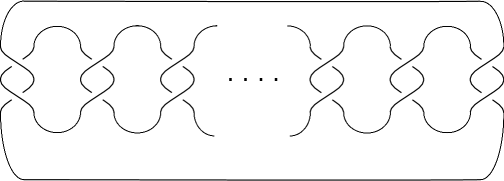
Figure 1. Surgery presentation for $Y$ and handle decomposition of $X$.

We are going to argue that $Y$ carries an open book decomposition with page a one–holed torus $S$ and monodromy $h$ when $S$ is suitably identified with $T$. In other words, $Y=Y_{(T,h)}$. Consider the picture on the left–hand side of Figure 2 for any $i\in\{2,\ldots,n\}$. The picture illustrates a one–holed torus $S$ embedded in the complement of the framed link $L$.

Proposition 4.1.

$S$ is the page of an open book decomposition on $Y$ which, under a suitable identification of $S$ with $T$, has monodromy $h$.

Proof.

The following proof is an adaptation to the present situation of the arguments given in [KM94]*Appendix. The surface $S$ can be isotoped to the one–holed torus $S^{\prime}$ illustrated in the picture on the right–hand side of Figure 2. To see that, just think about the fact that the complement of the Hopf link in $S^{3}$ is a torus times an interval. Moreover, the isotopy takes the oriented curves $\mu,\lambda\subset S$ in the left–hand picture to $\lambda^{\prime},-\mu^{\prime}\subset S^{\prime}$, respectively, illustrated in the right–hand picture. We could also enlarge slightly $S$ to $\tilde{S}$ and $S^{\prime}$ to $\tilde{S}^{\prime}$ so that $\partial\tilde{S}=\partial\tilde{S}^{\prime}$. We may identify $S$ and $S^{\prime}$ with $T$ so that the isotopy from $S$ to $S^{\prime}$ induces an orientation–preserving diffeomorphism $\phi\thinspace\colon T\to T$ prescribed, in terms of an oriented basis of $H_{1}(T;\mathbb{Z})$, by the matrix $M=\left(\begin{smallmatrix}0&-1\\ 1&0\end{smallmatrix}\right)\in SL(2;\mathbb{Z})$. Since the generators $x,y\in Diff^{+}(T,\partial T)$ associated to the given oriented basis correspond, respectively, to $\left(\begin{smallmatrix}1&1\\ 0&1\end{smallmatrix}\right)$ and $\left(\begin{smallmatrix}1&0\\ -1&1\end{smallmatrix}\right)$, one can easily check that $\phi=x^{-1}y^{-1}x^{-1}$.

2pt $c_{i-1}$ at 25 22 $\lambda$ at 55 160 $S$ at 65 100 $\mu$ at 225 160 $c_{i}$ at 220 22 $\mu^{\prime}$ at 435 160 $c_{i-1}$ at 460 22 $\lambda^{\prime}$ at 600 160 $S^{\prime}$ at 595 100 $c_{i}$ at 650 22

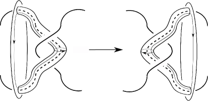
Figure 2. The isotopy from $S$ to $S^{\prime}$.

The same analysis applies to every clasp of $L$ except the one between the $1$–st and the $N$–th components of $L$. In that case, an analysis as above shows that matrix associated to the last isotopy is $-M=M^{-1}$ instead of $M$, corrisponding to the diffeomorphism $\phi^{-1}=xyx$.

Now we claim that, for each $i=1,\ldots,N$, there is another isotopy sending the surface $S^{\prime}:=D^{\prime}\cup A^{\prime}$, illustrated on the left–hand side of Figure 3, to the surface $S=D\cup A$ illustrated on the right–hand side. This isotopy goes through the solid torus glued along a neighborhood of the $i$–th component of $L$. In fact, it fixes $D$ and sends $A^{\prime}$ to $A$, sending the simple closed curve $\lambda^{\prime}\subset S^{\prime}$ to $\lambda^{\prime\prime}\subset S$, which twists $c_{i}$ times around $A$. To see this, recall that the presence of the framing coefficient “$c_{i}$” means that a neighborhood of the $i$–th component $L_{i}$ of $L$ with a meridian–longitude basis $m,\ell$ of its boundary is first cut out and then re–glued by sending $m$ to $c_{i}m+\ell$ and $\ell$ to $-m$. Thus, the simple closed curve $(\lambda^{\prime}\cap A^{\prime})\cup(\lambda^{\prime\prime}\cap A)$ bounds a meridional disk in the glued–up solid torus, while $A^{\prime}$ and $A$ can be identified with neighborhoods of parallel longitudinal curves on its boundary. This means that $A^{\prime}$ is isotopic to $A^{\prime\prime}$ via an isotopy which carries the annulus across the glued–up solid torus, sending $\lambda^{\prime}\cap A^{\prime}$ to $\lambda^{\prime\prime}\cap A$, and the claim is proved. As in the previous case of Figure 2, we may identify $S^{\prime}$ and $S$ with $T$ so that the isotopy induces an automorphism $T\to T$ represented by the matrix $N(c_{i})=\left(\begin{smallmatrix}1&c_{i}\\ 0&1\end{smallmatrix}\right)\in SL(2;\mathbb{Z})$, hence given by $x^{c_{i}}$.

2pt $\mu^{\prime}$ at 35 160 $c_{i-1}$ at 75 30 $A^{\prime}$ at 138 280 $\lambda^{\prime}$ at 203 220 $D$ at 195 100 $c_{i}$ at 255 30 $c_{i+1}$ at 342 30 $c_{i-1}$ at 605 30 $c_{i}$ at 685 30 $\lambda^{\prime\prime}$ at 735 230 $D$ at 740 100 $A^{\prime\prime}$ at 810 280 $c_{i+1}$ at 870 30 $\mu^{\prime\prime}$ at 900 155

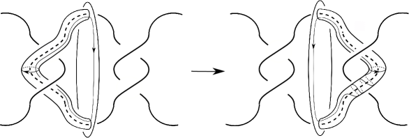
Figure 3. The isotopy from $S^{\prime}$ to $S^{\prime\prime}$.

By composing all the isotopies described so far, we see that $Y$ admits an open book decomposition with one–holed torus page, identified with $T$. The corresponding monodromy is obtained by composing the diffeomorphisms induced by the various isotopies. We do the calculation in terms of $x$ and $y$, starting from the first component $L_{1}$. Using the above analysis, denoting conjugation equivalence by $\sim$ and following our conventions on the composition of diffeomorphisms (see paragraph before Proposition 2.1) we obtain

$$x^{c_{1}}\phi x^{c_{2}}\cdots\phi x^{c_{N}}\phi^{-1}=x^{a_{1}+2}\phi(x^{2}\phi)^{b_{1}-1}x^{a_{2}+2}\cdots x^{a_{n}+2}\phi(x^{2}\phi)^{b_{n}-1}\phi^{-2}=\\ x^{a_{1}+1}y^{-b_{1}}\cdots x^{a_{n}}y^{-b_{n}+1}x^{2}yx\sim xyx^{2}yxx^{a_{1}}y^{-b_{1}}\cdots x^{a_{n}}y^{-b_{n}}=(xy)^{3}x^{a_{1}}y^{-b_{1}}\cdots x^{a_{n}}y^{-b_{n}}=h.$$

∎

By Proposition 4.1 we can view Figure 1 as a presentation of $Y_{(T,h)}$, including the induced open book decomposition. On the other hand, we can also view the framed link $L$ as prescribing the attachment of $n$ four–dimensional 2–handles to the 4–ball $B^{4}$, resulting in a smooth oriented 4–manifold $X$ with boundary orientation–preserving diffeomorphic to $Y_{(T,h)}$. Moreover, note that $L$ is a characteristic sublink of itself, i.e. $\operatorname{lk}(L,L_{i})=\operatorname{lk}(L_{i},L_{i})\bmod 2$ for each component $L_{i}\subset L$. Recall [GS99]*§5.7 that there is a natural one–to–one correspondence between Spin structures on $Y_{(T,h)}$ and characteristic sublinks of $L$, given by assigning to a Spin structure $\Theta$ the sublink $C$ of $L$ consisting of all components $L_{i}$ such that $\Theta$ does not extend across the 2–handle in $X$ attached to $L_{i}$. Moreover, by [EO08]*Lemma 6.1 the Euler class of $\xi_{(T,h)}$ vanishes, therefore $\xi_{(T,h)}$ is trivial as a 2–plane bundle over $Y_{(T,h)}$. Homotopy classes of trivializations of $\xi_{(T,h)}$ are in 1–1 correspondence with homotopy classes of maps $Y_{(T,h)}\to S^{1}$. If $Y_{(T,h)}$ is a rational homology 3–sphere we have $H^{1}(Y_{(T,h)};\mathbb{Z})=0$, therefore $\xi_{(T,h)}$ admits a unique trivialization up to homotopy. Moreover, each trivalization of $\xi_{(T,h)}$ canonically determines a trivialization of $TY_{(T,h)}$, hence a Spin structure on $Y_{(T,h)}$. We denote by $\Theta_{\xi}$ the Spin structure on $Y_{(T,h)}$ associated in this way to $\xi$. The following lemma is an adaptation to the present situation of [KM94]*Lemma A.6.

Lemma 4.2.

The Spin structure $\Theta_{\xi}$ corresponds to $L$ viewed as a characteristic sublink of itself.

Proof.

Let $L_{i-1}\subset L$ be any component of $L$, and $\mu$ an oriented meridian of $L_{i-1}$ sitting on a page $S$ of the open book decomposition of Proposition 4.1, as illustrated in the left–hand side of Figure 2. Since $\xi_{(T,h)}$ is compatible with the open book decomposition, up to homotopy we may assume that the trivialization of $TY_{(T,h)}$ associated to a trivialization of $\xi_{(T,h)}$ restricts to $\mu$ as the tangent to $\mu$ followed by the normal to $\mu$ in $S$ and the normal to $S$. This framing of $TY_{(T,h)}|_{\mu}$ has a natural stabilization to a framing of $TX|_{\mu}$, and as such it does not extend to the cocore of the 2–handle attached to $L_{i-1}$, therefore $L_{i-1}$ belongs to the characteristic sublink corresponding to $\Theta_{\xi}$. Since the same argument holds for each component of $L$, the statement is proved. ∎

For each component $L_{i}$ of $L$ there is a 2–sphere $S_{i}$ smoothly embedded in $X$, obtained as the union of a 2–disc properly embedded in $B^{4}$ with boundary $L_{i}$, with the core of the 2–handle attached along $L_{i}$ with framing $c_{i}$. We fix an orientation of $L$ by orienting each component of $L$ in anti–clockwise fashion in the diagram of Figure 1. This orientation of $L$ prescribes on orientation of each $S_{i}$ such that, if $v_{i}\in H_{2}(X;\mathbb{Z})$ denotes the corresponding 2–homology class, the classes $v_{1},\ldots,v_{N}$ form a basis of $H_{2}(X;\mathbb{Z})$ and intersect as follows:

(4.2) $$v_{i}\cdot v_{j}=\begin{cases}c_{i}&\text{if $i=j$}\\ -1&\text{if $\{i,j\}\neq\{1,N\}$ and $|i-j|=1$}\\ 1&\text{if $\{i,j\}=\{1,N\}$}\end{cases}$$

Using this, it is also easy to check that the homology class

(4.3) $$w:=\sum_{i=1}^{N}v_{i}\in H_{2}(X;\mathbb{Z})$$

is characteristic, that is $w\cdot\alpha\equiv\alpha\cdot\alpha\bmod 2$ for every $\alpha\in H_{2}(X;\mathbb{Z})$. The following lemma will be used in the proofs of Propositions 4.4 and 5.2.

Lemma 4.3.

Let $(\Lambda,\cdot)$ be an intersection lattice of rank $N\geq 2$. Suppose that $v_{1},\ldots,v_{N}$ is a basis of $\Lambda$ satisfying (4.2) with $c_{1},\ldots,c_{N}\geq 2$. Then, $(\Lambda,\cdot)$ is positive definite.

Proof.

Let

$$\xi=\sum_{i=1}^{N}x_{i}v_{i}\in\Lambda,\quad x_{1},\ldots,x_{N}\in\mathbb{Z}.$$

Since $c_{1}\ldots,c_{N}\geq 2$, we have

$$\xi\cdot\xi=\left(\sum_{i=1}^{N}x_{i}v_{i}\right)\cdot\left(\sum_{i=1}^{N}x_{i}v_{i}\right)=\sum_{i=1}^{N}x_{i}^{2}c_{i}-2\sum_{i=1}^{N-1}x_{i}\cdot x_{i+1}+2x_{1}x_{N}$$

$$\geq 2\sum_{i=1}^{N}x_{i}^{2}-2\sum_{i=1}^{N-1}x_{i}\cdot x_{i+1}+2x_{1}x_{N}$$

$$=(x_{1}-x_{2})^{2}+(x_{2}-x_{3})^{2}+\cdots+(x_{N-1}-x_{N})^{2}+(x_{N}+x_{1})^{2}\geq 0.$$

Moreover, $\xi\cdot\xi=0$ implies $x_{1}=\cdots=x_{N}=-x_{1}$, i.e. $\xi=0$. This shows that $(\Lambda,\cdot)$ is positive definite. ∎

Denote by $\mathbb{D}_{K}$ the intersection lattice $(\mathbb{Z}^{K},-I)$, i.e. the standard diagonal negative definite intersection lattice of rank $K$.

Proposition 4.4.

Let $h$ be an element of $Diff^{+}(T,\partial T)$ which can be written as:

$$h=(xy)^{3}x^{a_{1}}y^{-b_{1}}\cdots x^{a_{n}}y^{-b_{n}}\quad a_{i},b_{i},n\geq 1.$$

If $\xi_{(T,h)}$ is Stein fillable, then there is an isometric embedding of intersection lattices

$$\varphi:Q_{-X}:=(H_{2}(-X;\mathbb{Z}),\cdot)\hookrightarrow\mathbb{D}_{K},$$

where $K=\sum_{i=1}^{n}a_{i}+4$. Morever, $\varphi$ sends the element $w$ of (4.3) to a characteristic element.

Proof.

Given a Stein filling $(W,J)$ of $(Y_{(T,h)},\xi_{(T,h)})$ we can form the smooth, closed, oriented 4–manifold $M:=W\cup(-X)$. Proposition 2.1 and Lemma 4.3 imply that the intersection lattice $Q_{M}:=(H_{2}(M;\mathbb{Z}),\cdot)$ is negative definite, therefore by Donaldson’s theorem [Do87]*Theorem 1 $Q_{M}$ is isomorphic to the standard diagonal intersection lattice of the same rank: $Q_{M}\cong\mathbb{D}_{K}$, where $K=b_{2}(M)$. Moreover, in view of Proposition 2.1, we have $b_{2}(W)=exp(h)-2=\sum_{i=1}^{n}a_{i}-\sum_{i=1}^{n}b_{i}+4$, therefore

$$b_{2}(M)=b_{2}(W)+b_{2}(-X)=exp(h)-2+N=4+\sum_{i=1}^{n}a_{i}.$$

In particular, there is an isometric embedding $\mathbb{Q}_{-X}\hookrightarrow\mathbb{D}_{K}$. This proves the first part of the statement. Since the class $w$ defined by (4.3) is characteristic, its reduction modulo $2$ is represented by a closed surface $\Sigma_{w}\subset X$ dual to the second Stiefel–Whitney class $w_{2}(X)$. Then, $X\setminus W$ admits a spin structure $\mathbf{s}$ whose restriction to $\partial X=Y_{(T,h)}$ corresponds to $L$ viewed as a characteristic sublink of itself, and therefore equals $\Theta_{\xi}$ according to Lemma 4.2. But $\Sigma_{w}$ can be chosen to be an oriented surface representing an integral lift of $w_{2}(X)$ which is the first Chern class $c_{1}(\mathbf{s}_{w})$ of the unique extension of $\mathbf{s}$ to all of $X$ as a Spin^c structure $\mathbf{s}_{w}$. By construction, the restriction of $\mathbf{s}_{w}$ to $\partial X$ is $\Theta_{\xi}$. Therefore, since the Spin^c structure $\mathbf{s}_{J}$ on $W$ induced by the complex structure also restricts as $\Theta_{\xi}$ to $\partial W=\partial(-X)$, there is a Spin^c structure $\mathbf{s}_{M}=\mathbf{s}_{J}\cup\mathbf{s}_{w}$ on $M$ whose first Chern class $c_{1}(\mathbf{s}_{M})$ vanishes on $W$ by Proposition 2.1 and restricts to $X$ as $c_{1}(\mathbf{s}_{w})$. This shows that $\varphi(w)$ is the Poincaré dual of $c_{1}(\mathbf{s}_{M})$ and therefore is characteristic. ∎

5. The proof of Theorems 2.3 and 1.1

In this section we first derive some crucial consequences from Proposition 4.4 and then we use them to prove Theorems 2.3 and 1.1.

Let $v_{1},\ldots,v_{N}$ be the basis of $Q_{-X}$ chosen as in the previous section and satisfying (4.2). Let $\varphi$ denote an isometric embedding as in Proposition 4.4, and denote by $\overline{w}\in\mathbb{D}_{K}$ the image of $w=\sum_{i=1}^{N}v_{i}\in Q_{-X}$ under $\varphi$. The element $\overline{w}$ has the same square as $w$, that is

(5.1) $$\overline{w}\cdot\overline{w}=w\cdot w=\sum_{i=1}^{n}(a_{i}+2)+2\sum_{i=1}^{n}(b_{i}-1)-2(\sum_{i=1}^{n}b_{i}-1)+2=4+\sum_{i=1}^{n}a_{i}=K.$$

Since $\overline{w}$ is characteristic, there is a basis $e_{1},\ldots,e_{K}\in\mathbb{D}_{K}$ such that $e_{i}\cdot e_{i}=-\delta_{ij}$ for every $i,j$ and $\overline{w}=\sum_{i=1}^{K}e_{i}$. Let $\overline{v}_{1},\ldots,\overline{v}_{N}\in\mathbb{D}_{K}$ be the images of, respectively, $v_{1},\ldots,v_{N}$ under $\varphi$. We can define a $K\times N$ matrix $M=(m_{ij})$ by expressing each vector $\overline{v}_{j}$ in terms of the $e_{i}$’s:

(5.2) $$\overline{v}_{j}=\sum_{i=1}^{K}m_{ij}e_{i},\quad j=1,\ldots,N.$$

Observe that, since $\overline{w}=\sum_{i=1}^{N}\overline{v}_{i}$, we have

(5.3) $$\overline{w}\cdot\overline{v}_{i}=\begin{cases}\overline{v}_{i}\cdot\overline{v}_{i}&\text{if $i\in\{1,N\}$},\\ \overline{v}_{i}\cdot\overline{v}_{i}+2&\text{if $i\not\in\{1,N\}$}.\end{cases}$$

Lemma 5.1.

Let $M=(m_{ij})$ be the $K\times N$ matrix defined by (5.2).

1. For each $j\in\{2,\ldots,N-1\}$ there is a unique index $\tau(j)\in\{1,\ldots,K\}$ such that
   $m_{\tau(j)j}\in\{-1,2\}$;

2. For each $(i,j)\in\{1,\ldots,K\}\times\{1,N\}$ and for each $(i,j)\in\{1,\ldots,K\}\times\{2,\ldots,N-1\}$ with $i\neq\tau(j)$ we have $m_{ij}\in\{0,1\}$.

Proof.

Note that for every $(i,j)\in\{1,\ldots,K\}\times\{1,\ldots,N\}$ we have

$$m_{ij}(m_{ij}-1)=\begin{cases}0&\text{if $m_{ij}\in\{0,1\}$},\\ 2&\text{if $m_{ij}\in\{-1,2\}$}\end{cases}$$

and $m_{ij}(m_{ij}-1)>2$ if $m_{ij}\not\in\{-1,0,1,2\}$. Now, if $j\in\{1,N\}$ by (5.3)

$$\sum_{i=1}^{N}m_{ij}^{2}=-\overline{v}_{j}\cdot\overline{v}_{j}=-\overline{w}\cdot\overline{v}_{j}=-\left(\sum_{i}^{K}e_{i}\right)\cdot\left(\sum_{i}^{K}m_{ij}e_{i}\right)=\sum_{i}^{K}m_{ij},$$

therefore

(5.4) $$\sum_{i=1}^{K}m_{ij}(m_{ij}-1)=0.$$

Equation (5.4) implies that $m_{ij}\in\{0,1\}$ when $(i,j)\in\{1,\ldots,K\}\times\{1,N\}$. Similarly, when $(i,j)\in\{1,\ldots,K\}\times\{2,\ldots,N-1\}$ from (5.3) we obtain

$$\sum_{i=1}^{K}m_{ij}(m_{ij}-1)=2,$$

which implies that there is a unique index $\tau(j)$ such that $m_{\tau(j)j}\in\{-1,2\}$, while for $i\neq\tau(j)$ we must have $m_{ij}\in\{0,1\}$. ∎

Proposition 5.2.

Let $(c_{1},\ldots,c_{N})$ be the $N$–tuple defined in (4.1), $N\geq 2$. Then, there is a sequence of blowups $(s_{1},\ldots,s_{N})\rightarrow\stackrel{{\scriptstyle\text{blowup}}}{{\cdots}}\rightarrow(0,0)$ such that $c_{1}\geq s_{1},\ c_{2}\geq s_{2},\ \ldots,c_{N}\geq s_{N}$.

Proof.

If $N=2$ there is nothing to prove. Hence, I will assume $N\geq 3$. Let $M=(m_{ij})$ be the $K\times N$ matrix defined by (5.2). For each $i=1,\ldots,K$ we have

(5.5) $$\sum_{j=1}^{N}m_{ij}=-e_{i}\cdot\sum_{j=1}^{N}\overline{v}_{j}=-e_{i}\cdot\overline{w}=-e_{i}\cdot\sum_{k=1}^{N}e_{k}=1.$$

Note that, by Lemma 5.1 and (5.5), if a row of $M$ contains more than one nonzero entry then one of those entries equals $-1$. On the other hand, by Lemma 5.1 at most $N-2$ entries of $M$ are equal to $-1$. But since $\exp(h)=2+K-N\geq 2$, we have $K\geq N$, i.e. the matrix $M$ has at least $N$ rows. We conclude that a row $R$ of $M$ has a single nonzero entry, which by (5.5) must be equal to $1$. Deleting $R$ from $M$ we obtain a new matrix $M^{\prime}=(m^{\prime}_{ij})$ having $K-1$ rows and $N$ columns. The $m^{\prime}_{ij}$’s still satisfy (5.5). Moreover, we can use the $m^{\prime}_{ij}$’s as in (5.2) to define elements $\overline{v}^{\prime}_{j}\in\mathbb{D}_{K-1}$, $j=1,\ldots,N$. Note that $\overline{w}^{\prime}:=\sum_{j=1}^{N}\overline{v}^{\prime}_{j}$ and the $\overline{v}^{\prime}_{j}$’s intersect as in (5.3). Therefore the proof of Lemma 5.1 goes trough and, since $K-1\geq N-1>N-2$, we can reapply the argument just used to conclude that a row of $M^{\prime}$ has a single nonzero entry equal to $1$. Then we can delete that row obtaining a new matrix, reapply the same argument and so on. If we keep going this way until we can, i.e. until we obtain a matrix $M^{\prime\prime}$ with $N-2$ rows and $N$ columns, the elements $\overline{v}^{\prime\prime}_{1},\ldots,\overline{v}^{\prime\prime}_{N}\in\mathbb{D}_{N-2}$ defined by the columns of $M^{\prime\prime}=(m^{\prime\prime}_{ij})$ will satisfy

(5.6) $$v^{\prime\prime}_{i}\cdot v^{\prime\prime}_{j}=\begin{cases}-1&\text{if $\{i,j\}=\{1,N\}$}\\ 1&\text{if $\{i,j\}\neq\{1,N\}$ and $|i-j|=1$}.\end{cases}$$

In view of Lemma 4.3 we must necessarily have $\overline{v}^{\prime\prime}_{j}\cdot\overline{v}^{\prime\prime}_{j}=-1$ for some $j\in\{1,\ldots,N\}$. In particular $m^{\prime\prime}_{ij}=\pm 1$ for some $i$ and $m^{\prime\prime}_{sj}=0$ for $s\neq i$. Erasing the $i$–th row and the $j$–th column of $M^{\prime\prime}$ we get a matrix whose columns define $N-1$ elements of $\mathbb{D}_{N-3}$ which intersect as in (5.6). Since we are assuming $N\geq 3$, we can keep going in the same way until we have three elements in $\mathbb{D}_{1}$ intersecting each other in the usual way and having all square $-1$. Reconstructing backwards the various steps it is easy to check that $\overline{v}^{\prime\prime}_{1},\ldots,\overline{v}^{\prime\prime}_{N}\in\mathbb{D}_{N-2}$ have self–intersections $(-s_{1},\ldots,-s_{N})$, with $(s_{1},\ldots,s_{N})\rightarrow\stackrel{{\scriptstyle\text{blowup}}}{{\cdots}}\rightarrow(0,0)$, and that $c_{i}\geq s_{i}$ for each $i=1,\ldots,N$. This concludes the proof. ∎

Proof of Theorems 2.3 and 1.1.

If $N=1$ then $n=b_{1}=1$ and $h$ is clearly positive, therefore we may assume $N\geq 2$. As we recalled in Section 1, the fact that $(1)\Rightarrow(2)$ is well known. Moreover, by Proposition 3.3 we have the implication $(3)\Rightarrow(1)$ of Theorem 2.3 and by Proposition 5.2 we have $(2)\Rightarrow(3)$. This concludes the proof of Theorem 2.3, which together with Proposition 2.1 implies Theorem 1.1. ∎

Remark 5.3.

As pointed out by John Etnyre [Epc13], the fact that there exist Stein fillable, non–positive open books $(\Sigma,h)$ of any genus $g(\Sigma)\geq 2$ can be proved as follows. Let $(\Sigma_{1},f_{1})$ be any positive open book with $\Sigma_{1}$ equal to a one–holed torus, and let $(\Sigma_{2},f_{2})$ be one of the Stein fillable, non–positive examples from [Wa09] or [BEV10] with $g(\Sigma_{2})=2$. Consider a boundary connected sum $(\Sigma=\Sigma_{1}\natural\Sigma_{2},f_{1}\natural f_{2})$ (it doesn’t matter which component of $\partial\Sigma_{2}$ is involved in the sum). Then, $\xi_{(\Sigma,f_{1}\natural f_{2})}$ is the contact connected sum of $\xi_{(\Sigma_{1},f_{1})}$ and $\xi_{(\Sigma_{2},f_{2})}$ and therefore $(\Sigma,f_{1}\natural f_{2})$ is Stein fillable. Moreover, there is a properly embedded arc $a\subset\Sigma$ with endpoints on the same boundary component $C$ of $\partial\Sigma$, such that the an open neighborhood $N$ of $a\cup C$ in $\Sigma$ is a pair of pants whose complement is homeomorphic to the disjoint union of $\Sigma_{1}$ and $\Sigma_{2}$. By construction $f_{1}\natural f_{2}$ has a representative which restricts to $N$ as the identity. Suppose by contradiction that $f_{1}\natural f_{2}$ can be written as a composition of right–handed Dehn twists $\delta_{C_{1}}\circ\cdots\circ\delta_{C_{k}}$. It is easy to check that if $C_{i}\cap a\not=\emptyset$ for some $i\in\{1,\ldots,k\}$, then the arc $a$ is sent by $f_{1}\natural f_{2}$ “to the right” in the sense of [HKM07]. On the other hand, by construction $f_{1}\natural f_{2}(a)=a$, which is not to the right of $a$. This implies that $C_{i}\cap a=\emptyset$ for each $i$, and therefore $f_{1}\natural f_{2}=P_{1}\natural P_{2}$, where $P_{i}:\Sigma_{i}\to\Sigma_{i}$, $i=1,2$, is a positive diffeomorphism. But the map $(f_{1},f_{2})\mapsto f_{1}\natural f_{2}$ is a group homomorphism, thus applying [PR00]*Corollary 4.2 (iii) one can easily show that it is injective. We conclude that $f_{2}$ is positive, contrary to the initial assumption. Repeating the same construction sufficiently many times one can construct Stein fillable, non–positive open books with pages of any genus strictly bigger than one.