Galactic Interaction as the Trigger for the Young Radio Galaxy MRC B1221$-$423

Abstract

Mergers between a massive galaxy and a small gas-rich companion (minor mergers) have been proposed as a viable mechanism for triggering radio emission in an active galaxy. Until now the problem has been catching this sequence of events as they occur. With MRC B1221$-$423 we have an active radio galaxy that has only recently been triggered, and a companion galaxy that provides the “smoking gun”. Using spectroscopic data taken with the VIMOS Integral Field Unit detector on the European Southern Observatory’s Very Large Telescope, we have examined the distribution, ionization state and kinematics of ionized gas in this interacting system. We have also modelled the stellar continuum with synthesised spectra of stellar populations of different ages. From our study of the ionized gas, we have derived preliminary models for the geometry of the interaction, analysed the kinematic behaviour of the ionized gas, and examined the ionization mechanisms at work throughout the system. Our modelling of the stellar continuum allowed us to identify and date distinct stellar populations within the galaxy pair. We find evidence of multiple episodes of widespread starburst activity, and by dating these populations, we provide tentative insight into the history of the interaction.

1 Introduction

One of the most dramatic but poorly understood stages in the evolution of galaxies is the formation of an Active Galactic Nucleus (AGN; henceforth used for both the singular and plural). This energetic phenomenon is thought to be powered by material accreting onto a supermassive black hole (SMBH) lying at the core of the host galaxy. It is now becoming clear that SMBHs and the galaxies they inhabit share an intimate co-evolutionary history, suggesting that the presence of an AGN affects the host galaxies in important and unexpected ways. Examples include modulation of star formation via radio-mode feedback (e.g. Silk and Rees 1998, Fabian 1999, King 2003), the SMBH-to-bulge mass relation (Ferrarese & Merritt 2000, Gebhardt et al. 2000, Di Matteo et al. 2005), and acting to enrich the IGM in metals (Germain et al. 2009, Barai et al. 2011), energetic particles (Ginzburg & Syrovatskii 1965, Hillas 1984), and magnetic fields (Jafelice et al. 1992, Kronberg et al. 2001, and references therein). The processes occurring in AGN are thus thought to play a fundamental role in driving the evolution and ecology of galaxies.

Among the most significant gaps in our current understanding of AGN is the triggering phase of the activity. A number of different mechanisms may be responsible for AGN triggering, ranging from internal stochastic processes in relatively low luminosity AGN (Ballantyne et al. 2006; Hasinger 2008; Hopkins & Hernquist 2009; Lutz et al. 2010) through to full-scale galactic mergers in the most luminous examples (e.g. Barnes & Hernquist 1991; Mihos & Hernquist 1996). To determine the relative importance of environmental and internal processes will require spatially resolved studies of large samples of galaxies hosting an AGN. Two upcoming surveys will address this need: the CALIFA survey (Sánchez et al. 2012) will perform integral field unit (IFU) observations of a statistically well-defined sample of over 600 galaxies, while the SAMI survey (Croom et al. 2012) will bring a powerful new combination of multi-object and IFU spectrograph technology to bear on the study of over 5000 galaxies in a range of environments.

To date, arguably the most well studied and robust of the proposed triggering mechanisms is the merger scenario. This model proposes that gravitational interaction between two galaxies triggers a large amount of gas to migrate to the core of the host galaxy, where it forms an accretion disk around the SMBH in the galactic nucleus. The hot accretion disk and the charged particles accelerated as a direct result of the accretion process are then responsible for the prodigious power output that we observe.

A number of lines of evidence provide support for the merger hypothesis. For example, AGN hosts have been found to often display disturbed morphologies (Longair et al. 1995; Best et al. 1996, Koss et al. 2010, Mezcua et al. 2012), and show evidence of significant bursts of ongoing or recent global star formation (Veilleux 2001, and references therein; Mezcua et al. 2012). These properties are generally interpreted as arising from gravitational interaction with a neighbouring galaxy. In addition, a number of statistical studies have pointed to a tendency for AGN hosts to reside in over-dense regions or alongside companion galaxies of comparable size (e.g. Koss et al. 2010). Though these observations would seem to imply that galaxy mergers play an important role in AGN triggering, the evidence is not completely clear-cut. For example, recent studies have found no clear evidence for increased merger rates or an excess of nearby companions for typical AGN hosts (e.g. Miller et al. 2003, Grogin et al. 2005, Li et al. 2006, Gabor et al. 2009). Recently, even the correlation between a galaxy’s AGN-hosting status and the level of morphological disturbance it shows have been called into question by Cisternas et al. (2011). Each of the studies above seem to indicate either zero or weak association between AGN activity and the host galaxy’s environment or morphology. It is difficult to explain these results if the majority of AGN are triggered through mergers between galaxies of comparable mass (so-called ‘major mergers’).

In part to address the inconsistencies outlined above, it has been suggested that so-called minor mergers (often defined as mergers between galaxies with a mass ratio of  $\buildrel<\over{\sim}$ 1:3 — see Stewart 2009; Lotz et al. 2011) may play a significant role in triggering AGN activity (e.g. Taniguchi 1999). This scenario proposes that an AGN can be triggered by interactions between a large host galaxy and a dwarf companion, and it directly addresses several of the objections to the major merger model raised above. Minor mergers are known to be strongly associated with kinematic disturbances that can trigger activity such as starbursts in the host galaxy (e.g. López-Sánchez 2010). It appears that most galaxies are orbited by small companions (e.g. Zaritsky et al. 1997), and computational modelling shows that minor mergers should be efficient at driving gas into the core regions of the dominant galaxy in such scenarios (Hernquist & Mihos, 1995). However, the same characteristics that make minor mergers desirable from a theoretical point of view make them difficult to study observationally: Minor mergers produce intrinsically less disturbance to the host galaxy making them hard to identify morphologically, the systems will only appear disturbed for a shorter period of time, and minor companions are low mass objects by definition, making them intrinsically faint and more difficult to detect.

MRC B1221$-$423 is a system that has been identified as a massive galaxy that is undergoing a minor merger with a low mass gas-rich companion (Johnston et al. 2010). Furthermore, it contains a young compact steep spectrum (CSS) source with an estimated age of $\sim 10^{5}$ years (Safouris et al. 2003). The youth of the CSS source means that this AGN has only been triggered recently, and given that we now observe the system undergoing a minor merger, it represents an extraordinary laboratory for studying merger-induced AGN triggering. We obtained Integral Field Unit (IFU) spectroscopy of the system using the VIsible Multi Object Spectrograph (VIMOS) instrument on the Very Large Telescope (VLT) at the European Southern Observatory (ESO), Chile. Using this dataset, we were able to study the kinematics and ionization of the gas, as well as examine the ages of the constituent stellar populations, to arrive at a tentative model for the interaction.

Our spectroscopic study of the MRC B1221$-$423 system is presented as follows. In section 2 we describe our observations and data reduction. In section 3.1, we present results and analysis of the distribution and kinematics of the ionized gas. In section 3.2, we describe the results from modelling of the stellar continuum. In section 4, we discuss our results in the light of previous work done on this system, and present our conclusions. Throughout, we have assumed a flat $\Lambda$-CDM cosmology with $H_{0}=71$ km s${}^{-1}\$Mpc^-1, $\Omega_{M}=0.27$ and $\Omega_{\Lambda}=0.73$. At the redshift of the galaxy, 1 arcsec corresponds to a projected separation of 2.876 kpc.

2 Observations and Data Reduction

2.1 Observations

Service mode observations of the MRC B1221$-$423 system were carried out using the VIMOS instrument (Le Fèvre et al. 2003), mounted on the ‘UT3 Melipal’ telescope at the ESO VLT. The instrument was used in its IFU spectrographic mode.

The observations were taken in six separate observation blocks (OBs), on the nights of 2009-Dec-16, 2009-Dec-22 & 2010-Jan-10. Each OB consisted of two object exposures bracketing a single sky exposure. The object exposures in each OB were jittered to ensure full coverage of the system in the event of dead IFU fibres (hereafter, we will refer to single IFU fibres as ‘spaxels’). Integration times for the object and sky exposures were 1260 and 350 seconds respectively, giving a total on-object integration time of 252 minutes.

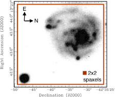
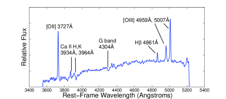
Figure 1: a) The spatial coverage of our VIMOS IFU observations delimited by the red box; the spaxel scale is defined by a solid red square. East is up and North is to the right. Image pixel scale is that of the NTT optical image. The MRC B1221$-$423 system can be seen in the North-East corner. The bright object in the South-West of the frame is a Galactic star. b) Spectral coverage of our observations, showing a spectrum of the nuclear region of the MRC B1221$-$423 system, with wavelengths given in the rest frame of the system ($z=0.1706$). The spectrum is a composite of 20 spaxels covering the nuclear region. The y-axis scale is in arbitrary units.

Our observations utilised the instrument in its low spatial resolution mode coupled with the HR Blue grism. This configuration yields a $40\times 40$ spaxel IFU head for a total number of 1600 spaxels, with a spatial resolution of $0.67^{\prime\prime}$ per spaxel and a spectral resolution of 2 Å at the central wavelength of the grism. The resulting field of view (FOV) covered $27^{\prime\prime}\times 27^{\prime\prime}$ on the sky (Figure 1a), while the spectral coverage was 4150-6200Å  corresponding to $\sim$3550-5220Å in the rest frame of the target galaxy (Figure 1b). Data in each OB were taken when the sky transparency was ‘clear’, the seeing FWHM was $<1.2^{\prime\prime}$, the moon illumination $<0.7$ (grey), and moon position $>30^{\circ}$ from the target galaxy.

In addition, a number of calibration frames were taken contemporaneously with the target observations. These included arc-lamp exposures, halogen lamp flats, bias frames and observations of spectrophotometric standard stars.

2.2 Data Reduction

The data reduction followed standard IFU reduction procedures as implemented in the VIMOS Interactive Pipeline Graphical Interface (VIPGI), a purpose-written program for reducing VIMOS data. The program itself and the data reduction procedures are described in detail in both Scodeggio et al. (2005) and the VIPGI User Manual. Briefly, the process involved bias correction, flat-fielding and wavelength calibration of the IFU images based on calibration data taken during observations. A spectrophotometric calibration was then applied to correct for variation in spectral sensitivity of the IFU system and obtain the absolute flux scale for the data. The spectra were then collapsed to 1D, extracted, and corrected for variation in the relative transmission of the IFU fibres. Finally, the data for each OB were assembled into a datacube based on a mapping between positions of fibres in the IFU head and spectra on the CCD.

We implemented the next step in our reduction process, the sky subtraction, outside the VIPGI environment. Due to the extended nature of our target, separate exposures of a nearby and relatively empty patch of sky were obtained in addition to the object exposures. The sky subtraction was applied to data in each OB separately, using the following procedure:

1. The calibrated data from each of the 1600 spectra forming the sky exposure for a given OB were sorted according to the integrated flux and noise levels over a defined region of the spectrum. The median 10% were retained while the rest were discarded, eliminating any sky spectra recorded by fibres with poor transmission characteristics.

2. The 160 retained spectra were averaged to form a ‘master’ sky spectrum.

3. The master spectrum was individually scaled to each of the spaxels in the two object exposures in each OB, based on the strength of the prominent [O I]$\lambda$5577 sky emission line.

4. The sky spectrum was subtracted from the object spectra.

Data from individual OBs were aligned using their World Coordinate System (WCS) header information and stacked to yield the final product datacube. To assess the accuracy of the WCS alignment, we also manually calculated the offsets between exposures based on the position of a bright star located fortuitously in the FOV (Figure 1a). The accuracy of the alignment was then assessed for both methods by collapsing the stacked datacube along the spectral axis and examining the 2D autocorrelation function of the resulting image. The alignment based on the WCS headers was found to be at least as accurate as the manual determination.

A correction for Galactic reddening was then applied to the data with $A_{V}=0.331$ mag. (Schlegel et al. 1998). The Calzetti et al. (2000) recipe was used for this purpose, being specifically formulated to de-redden the spectra of starburst galaxies. The formulation states that given an observed spectrum $f_{obs}(\lambda)$ and a reddening coefficient $A_{V}$, we can calculate the de-reddened spectrum, $f_{int}(\lambda)$, using the relations:

$$f_{int}(\lambda)=\frac{f_{obs}(\lambda)}{10^{-0.4A_{\lambda}}},$$

where

$$A_{\lambda}=\frac{A_{V}}{4.05}[2.659(-2.156+\frac{1.509}{\lambda}-\frac{0.198}{\lambda^{2}}+\frac{0.011}{\lambda^{3}})+4.05].$$

An additional correction for reddening internal to the MRC B1221$-$423 system was made using the same formulation and estimates of $A_{V}$ made by Johnston et al. (2005). We applied a correction across the field based on their estimated $A_{V}$ map, which ranged from close to 0 for many parts of the system, to $\sim 1$ for the knotty star-forming regions and the companion, and up to 3 for the inner nucleus. We note here that in section 3.3.1 where we model the stellar continuum, we allow $A_{V}$ to be a semi-free parameter in the fit of intrinsic reddening to the uncorrected data. We find that the values used for $A_{V}$ for our intrinsic reddening correction described above for the various regions in the system come close to providing the optimal fit between the stellar models and data. This provides some level of a posteriori confirmation of the $A_{V}$ values we adopt from Johnston et al. (2005).

3 Results

3.1 Ionized Gas

Our observations allowed us to study the 2-dimensional distribution, kinematics and ionization levels of the ionized gas across the MRC B1221$-$423 system. To characterise the gaseous emission, Gaussian profiles were fitted to prominent emission lines in the datacube in a semi-automated fashion, using scripts developed for this purpose (provided by R. Sharp, private communication, July 2010). This software uses an IDL implementation of the AMOEBA downhill simplex fitting algorithm (Press et al. 2007). Each line was fitted in isolation using a standard four parameter Gaussian model:

$G=A_{0}\exp(-x^{2}/2)+A_{3}$,

where $x=(\lambda-A_{1})/A_{2}$, $A_{0}$ determines the amplitude of the Gaussian peak, $A_{1}$ its central wavelength, $A_{2}$ its width, and $A_{3}$ the continuum level. Suitable line and continuum fitting constraints were defined in advance of fitting. Line fitting was assessed via a simple comparison of the $\chi^{2}$ fits of the data with the emission-line model and a constant continuum model. After fitting, 2-D line maps of the full field were formed.

Where strong discontinuities were observed, the fitted spectra were examined visually to check for accuracy and whether fitted features were genuine. In this way, fits were derived for the [O III]$\lambda$5007, [O III]$\lambda$4959, H$\beta$ and [O II]$\lambda$3727 emission lines for each of the 1600 spectra comprising the datacube.

Single Gaussian profiles were generally found to provide accurate fits to the line profiles across most of the face of the system. The exception was the high excitation [O III] doublet in the innermost $\sim$6 kpc of the nuclear regions. A routine capable of fitting two Gaussian components was found to provide a superior fit. However, detailed interpretation of the gaseous kinematics that this implies is beyond the scope of this paper.

With the fitting procedure completed, the fit parameters were recorded along with associated spatial positions and spectral lines. These included the peak amplitude, peak position, flux under the line at full-width zero-intensity, line width at full-width half-maximum, and the continuum flux density on either side of the line.

3.1.1 Distribution of Ionized Gas

Spatial maps of the emission intensity across the system were made for each of the major emission lines in the spectral range. Figure 2 shows the spectral line contours overlaid on the V-band optical image.

The strongest overall emission feature in the spectral region observed is the [O II]$\lambda$3727 line (Fig. 2c). The [O II] emission intensity peaks strongly in the nuclear region of the galaxy, but significant emission is seen throughout the system, most notably in the vicinity of the nucleus, the bright knotty complexes to the west, and the companion galaxy. Notwithstanding its limitations, [O II] emission is often used as a tracer of star formation in galaxy systems, and the relative strength of this emission line throughout much of the MRC B1221$-$423 system is suggestive of widespread ongoing star formation.

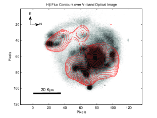
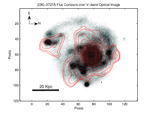
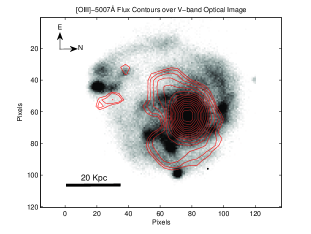
Figure 2: a) V-band NTT image of the MRC B1221$-$423 system in greyscale. The axis scales in the subsequent images correspond to the pixel numbers in this NTT image, with overlaid logarithmic contours, spaced by $\sqrt{2}$, as follows: b) H$\beta$ emission, over the interval 0.3 to 5.0 $\times 10^{-16}$ erg s^-1 cm^-2, c) [O II]$\lambda$3727 emission, over the interval 1.0 to 36.0 $\times 10^{-16}$ erg s^-1 cm^-2, d) [O III]$\lambda$5007 emission, over the interval 0.3 to 18.4 $\times 10^{-16}$ erg s^-1 cm^-2. All IFU data have been spatially smoothed with a $3\times 3$ spaxel boxcar.

H$\beta$ emission (Figure 2b) is also found widely throughout the system, and represents the strongest emission outside the nucleus. The emission is strongly correlated with the bright knotty complexes, which superficially take on the appearance of star-forming regions embedded in spiral arms. It is well known, however, that the host galaxies of CSS sources have absolute magnitudes consistent with first-ranked ellipticals, and frequently show evidence of interactions (eg. O’Dea 1998), with linear features that can mimic spiral arms. Moreover, the H$\beta$ emission does not appear to match the optical emission seen sweeping from the companion towards the host galaxy to the east of the nucleus. The morphology and location of this feature is suggestive of a tidal tail being pulled out as a consequence of the gravitational interaction between host and companion. We speculate that this tidal debris may wrap completely around the host galaxy, forming a continuous shell of material with the knotty regions to the west of the nucleus (see the toy model presented in section 3.2.2). If so, the entire shell may represent gas and dust that has been fed into the host after being tidally stripped from the companion. An alternative possibility is that the shell may have been pulled out of the companion by ram-pressure stripping as it passed through the extended regions of the host on its orbit.

The fact that the H$\beta$ and V-band emission are not spatially coincident in the tidal tail is notable, given that the H$\beta$ line is typically associated with the presence of young stars. A speculative interpretation is that the tidal tail of stars seen in the V-band image is a relic of a previous orbit of the companion around the host, and is now gas poor after star formation and gas stripping during the ensuing period. The H$\beta$ emission would then trace the tidal tail pulled out by the companion during the current orbit, and which, not having had time to form stars in great numbers, is relatively dim in V-band emission. We investigate this possibility further in section 3.3.2.

The [O III]$\lambda$5007 (Figure 2d) emission shows up primarily in the nucleus of the host galaxy. Given its ionization energy of 35.12eV, we would expect [O III] to be largely confined to the central regions of the host, where the hard UV continuum from the AGN is sufficiently intense, or to regions surrounding massive stars in star-forming regions. In addition to the nucleus, we detect significant levels of emission from two extended regions to the South-East and South-West of the nucleus. The region to the South-West may be correlated with the knotty complexes in the V-band image, but the emission to the South-East does not match any significant optical feature. This suggests the presence of high energy processes not associated with star formation occurring in this region; we return to this point in the following section.

3.1.2 Ionization Levels in the MRC B1221$-$423 System

Since our wavelength coverage did not include all the lines used in the more commonly used emission-line diagnostics, we used a diagnostic diagram and associated classification scheme devised by Lamareille (2010). Briefly, the scheme can be used to differentiate between multiple AGN-like and star-formation processes, by plotting log([O III]/H$\beta$) versus log([O II]/H$\beta$). The classification regions are defined empirically, based on the observational characteristics of a large sample of extragalactic objects.

A correction for intrinsic reddening in the MRC B1221$-$423 system was first applied to the data, based on the Calzetti formulation (Calzetti et al. 2000) and estimates for the reddening parameter $A_{V}$ derived by Johnston et al. (2005).

Figure 3 shows the resulting diagram, with data points colour-coded according to their spatial association with optical features seen in V-band images (see inset, Figure 3). The data points separate cleanly into several distinct regions across the diagram, indicating that different ionization mechanisms are operating in different spatial locations across the galaxy. The knotty regions have line ratios consistent with those of star-forming galaxies, confirming the presence of ongoing star formation in these regions. Likewise, line ratios indicative of star formation are also found in the emission from the companion galaxy and tidal tail. The hypothesis that this galactic system is undergoing a gravitational interaction/merger is further supported by these results which indicate the presence of widespread active star formation throughout the system.

The nuclear region of the host galaxy maps to the LINER/Seyfert 2 regions of the plot, consistent with the object’s existing classification as a LINER galaxy. A small region of extended [O III] emission to the southeast of the nucleus (identified in section 3.1.1) maps to the regions of the plot indicating AGN-type processes. This suggests that higher energy processes operate in this region, potentially associated with the AGN activity. Possibilities may include hard-ultraviolet emission from the AGN accretion disk, shock-front ionization from fast nuclear outflows or jets, or shock ionization from gaseous inflows.

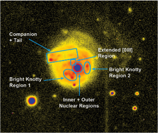
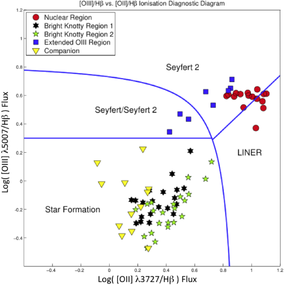
Figure 3: a) V-band image depicting the spatial regions from which the spaxels were drawn for the analysis in section 3.1.2. The false colour scheme was employed to maximise the contrast of distinct morphological features. b) Lamareille diagnostic diagram showing log([O III]/H$\beta$) versus log([O II]/H$\beta$) for regions in which these values are defined. The blue lines demarcate the diagnostic regions as defined by Lamareille (2010). The points separate out cleanly into star-formation and AGN-like processes, showing strong correlation between spatial location of the spaxel and the dominant ionization process at work in the region.

3.2 Integrated Emission Line Fluxes

In this section, we calculate the integrated flux for each of the three main emission lines in our spectra, both in specific regions of the interacting system and in the system as a whole. From this we estimate the global star-formation rates, H II mass and metallicity for those regions in which the diagnostic emission-line ratios indicate pure star formation and are not associated with AGN activity (see section  3.1.2).

The spatial regions adopted are identical to those used in our work on stellar continuum fitting and are described in section 3.3 below. Spaxels were summed from the nuclear region of the galaxy as defined in Fig. 6(region 6), while the two knotty regions, companion and extended [O III] region were all summed within the limits of the regions depicted in Fig. 7 (regions 3 & 4, 5 and 6 respectively).

The integrated line + continuum fluxes in each spatial region were obtained by summing the flux density over the relevant spectral regions for each line. A continuum band adjacent to the lines and with the same total spectral width, was then subtracted to yield the integrated emission line fluxes. Uncertainties were estimated from the noise in the continuum bands, with appropriate scaling to take account of the subtraction process. The H$\alpha$ luminosity was estimated by multiplying the H$\beta$ flux by 2.8 (the theoretical case-B Balmer decrement), assuming a luminosity distance of 770 Mpc.

We calculated the star formation rate (SFR) for each of the defined regions based on the relationship between H$\alpha$ and SFR described by Calzetti et al. (2007):

$${\rm SFR(M_{\odot}\,yr^{-1})}=5.3\times 10^{-42}L({\rm H}\alpha)_{corr}\,{\rm erg\,s^{-1}}.$$

We find a very high star-formation rate throughout the system, especially in the knotty blue regions described earlier. The uncertainty in the SFR quoted in Table 1 is based solely on the uncertainty in the H$\beta$ flux and does not take account of the significant uncertainty in the correction for intrinsic reddening in the galaxy (section  3.1.2). Nevertheless, the SFR is undoubtedly high, consistent with a gas-rich merger.

The H$\beta$ flux may also be used to calculate the H II mass of the galaxy using the relationship described by Pérez-Montero (2002):

$$M{\rm{}_{H\,II}(M_{\odot})}=1.485\times 10^{-35}L({\rm H}\alpha)_{corr}\times(n_{e}/100),$$

where $n_{e}$(cm^-3) is the electron density. As expected for a gas-rich merger, we find large reservoirs of ionised hydrogen, particularly in the knotty regions. As shown in section  3.2.1 below, this gas may be moving in large bulk flows through the system as a result of the merger process.

We include in Table 1 the gas-phase metallicities calculated using the iterative method of Kobulnicky & Kewley (2004); see also López-Sánchez & Esteban (2010). Most of the B1221$-$423 system possesses very similar O/H metallicity, between 8.4–8.8 for all regions examined assuming ‘lower branch’ metallicities, or around 9.0 for ‘upper branch’ metallicities. Without additional information from the [N II]/H$\alpha$ ratio, however, we are unable to determine which branch our object lies on.

Table 1: Integrated fluxes and derived quantities for selected regions of the MRC B1221$-$423 system (defined in section  3.3), corrected for reddening. Listed uncertainties are based on the estimated errors in the emission-line fits alone, and do not include uncertainties in the reddening correction. The two values given for the O/H abundance correspond to the lower- and upper-branch values respectively; see text.

			Flux ($10^{-16}$ erg s-1 cm-2)
Region	Spaxels	$A_{V}$	[O II]	H$\beta$	[O III]	Lamareille	$L({\rm H}\beta$)	SFR	$M_{\rm H\,II}$	12+log(O/H)
		mag.	$\lambda$3727		$\lambda$5007	(Fig. 3)	$10^{40}$ erg s-1	M⊙/yr	$10^{6}$ M⊙
Nucleus	16	2.5	$650\pm 15$	$49\pm 3$	$230\pm 4$	LINER/Sey	$34.9\pm 1.9$	—	—	—
Knotty reg.1	24	1	$71\pm 13$	$36\pm 4$	$14\pm 2$	SF	$25.3\pm 2.4$	$37.5\pm 1.3$	$70.8\pm 2.4$	8.51, 9.07
Knotty reg.2	30	2	$21\pm 3$	$8.9\pm 0.7$	$5.3\pm 0.6$	SF	$6.4\pm 0.5$	$9.5\pm 0.3$	$17.9\pm 0.5$	8.79, 9.03
Ext. [O III]	9	1.5	$13\pm 4$	$3.6\pm 3.1$	$12.3\pm 1.0$	Sey	$2.6\pm 2.4$	—	—	—
Companion	56	1	$10\pm 3$	$7.0\pm 0.7$	$7.6\pm 0.6$	SF	$5.0\pm 0.5$	$7.4\pm 0.3$	$14.0\pm 0.5$	8.44, 9.05
Whole system	396	varies	$790\pm 20$	$117\pm 6$	$298\pm 7$	All	$83\pm 4$	$>54$	$>103$	8.58, 9.05

3.2.1 Global Kinematics of the Ionized Gas

The kinematics of the gas and stars provides an important test of the merger hypothesis, yielding constraints on the possible geometry of the interaction. Safouris et al. (2003) used long-slit spectra taken at multiple position angles to estimate an overall rotational orientation and velocity for the system. Our full spectroscopic coverage across the face of the system allows us to take this further and infer the overall geometry of the interaction, as well as resolving the gaseous kinematics on smaller angular scales.

The reference frame adopted for the kinematic analysis was the redshift of the system ($z=0.1706$; Simpson et al. 1993). We computed the relative velocity of the ionized gas in each spaxel, adjusted to the heliocentric frame, and then created two-dimensional maps of the line-of-sight velocity as a function of spatial position across the system (Figure 4), using the usual colour conventions for recession and approach. It is, of course, also possible to define the reference velocity for each emission map in terms of the redshift of that emission line at the galactic nucleus. In doing so, it is immediately clear that there are significant differences between the two reference velocities. For a discussion of the difference between the systemic and nuclear emission-line redshifts, see Johnston et al. (2010).

The velocity maps resulting from our data show significant structure in each of the major emission lines in our wavelength range. Furthermore, each line shows a different velocity distribution, in some cases subtly different, and in others markedly so. The H$\beta$ velocity distribution shows a clearly defined rotational axis, with blueshifted regions to the southwest of the nucleus and redshifted regions to the northeast. Using the H$\beta$ data, we measure the position angle of the projected rotation axis to be $137^{\circ}\pm 5^{\circ}$ (see Fig. 4d). This differs slightly from the PA obtained by Safouris et al. (2003), who measured a PA of $118^{\circ}\pm 10^{\circ}$ with a more limited data set consisting of long-slit spectra. The apparent rotation is very smooth across the system, characteristic of a uniformly rotating disk or sphere of material. The largest relative velocity difference that we measure is $\sim$280 km s^-1. The fact that we see significant rotation through the entire system indicates that the companion is not orbiting in the plane of the sky, as it appears in optical images, but the rotation axis is significantly inclined to the line of sight.

In comparison with H$\beta$, the oxygen lines show greater complexity in their velocity structure. In [O II] we still see the same overall rotation as in H$\beta$ but the nuclear region shows more complexity. The most obvious deviation from the smooth H$\beta$ profile is the locally blueshifted region of gas wrapping around the host galaxy nucleus (see Fig. 4d), which we also observe in the [O III] emission. This feature appears to emerge out of the knotty region to the SW of the nucleus, skirting the nuclear region to the W and NW. We speculate that this structure may be associated with a large-scale flow of gas wrapping around from behind the nuclear region, moving up towards us on an orbital trajectory taking it around the nuclear region of the system. Alternatively, we may be seeing a region of local kinematic complexity in the gas, such as nuclear outflows, superimposed on the smooth underlying rotation profile. We note that the single Gaussians employed to fit these regions still provided an excellent fit to the emission lines, despite this apparent outflow structure. IFU data with higher spatial resolution will be used to investigate this in more detail.

We now digress briefly to consider how the kinematic results may affect our analysis in section 3.1.2. The fact that the different ionized species show different velocity structure implies that the emission originates from different spatial regions in the host system. We have therefore been careful to keep the interpretation of our line-ratio diagnostics in section 3.1.2 rather general. However, the sample of objects used to define the classification scheme in Lamareille (2010) might potentially be expected to possess similar ionization structure to MRC B1221$-$423. Given the scheme’s firm basis in empirical observation, valid over a diverse sample of objects, we believe that our general conclusions are justified. We now go on to discuss the kinematics described above in the context of plausible interaction geometries for this system.

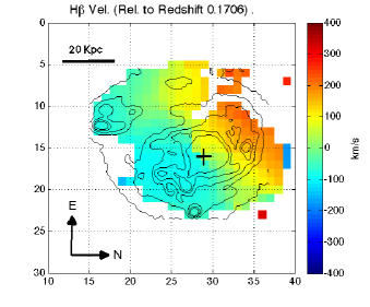
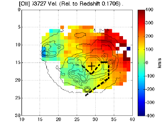
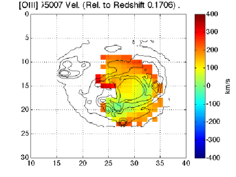
Figure 4: Colour-coded emission-line velocities for the system, relative to $z=0.1706$, overlaid with brightness contours from the $V$-band optical image. The axes refer to IFU spaxels, and a black cross denotes the position of the galactic nucleus. a) H$\beta$, showing a prominent rotation axis extending NW to SE through the system, and a smooth rotation profile. b) [O II]$\lambda$3727, with the projected rotation axis calculated from our IFU data using H$\beta$ emission superimposed as a solid line (PA = $137^{\circ}$); the rotation axis determined by Safouris et al. (2003) is shown as a dotted line (PA = $118^{\circ}$). c) [O II]$\lambda$3727, showing the blueshifted region described in the text, delimited with dotted lines. d) the [O III]$\lambda$5007, also showing a blue-shifted feature but no clear rotation.

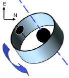
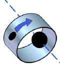
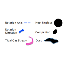
Figure 5: Two toy models for the orbital geometry of the MRC B1221$-$423 host and companion, inferred from the emission line velocity data. a) & b) show the two geometries for the companion’s orbit around the host allowed by the data, with the silver ’bands’ in place to make the orbital geometry clear. If the geometry depicted in b) is correct, then c) shows a possible explanation for the ‘disappearing’ tidal tail described in section 3.1.1, as well as the blueshifted feature seen wrapping around the nucleus in the oxygen lines (see figure 4d). In c), both of these features are generated by a gaseous tidal flow from the companion into the host.

3.2.2 Toy Models for the Interaction Geometry

The line-of-sight velocity data allow two possible rotational senses for the MRC B1221$-$423 system, and we now present toy models incorporating each. These models aim to describe qualitatively the most significant features observed in the kinematics and distribution of the gas. The first model is presented in Figure 5a. It shows the host nucleus, and the companion galaxy in orbit around it. The rotation axis extends through the host nucleus where most of the mass in the system is contained, running from the northwest to the southeast. In this scenario, the companion is moving towards us and down to the southwest, after having orbited around behind the system from our frame of reference. Referring back to Figure 2a,b, the H$\beta$ tidal tail would then arise as a result of being pulled out of the companion or host at or near their point of closest approach. The knotty star-formation regions could result from gas fed into the system or otherwise disturbed as the companion has moved around on its orbit.

There is a second viable alternative, broadly consistent with the data, that we could not rule out (Figure 5b,c). In this scenario, the companion is also moving towards us at present, but its orbit is directed around in front of the system towards the northeast. This picture is consistent with the velocity data, but possesses the additional advantage of being able to explain the observation that the tidal tail of H$\beta$ emission emanating from the companion disappears to the east of the host nucleus (see Figure 2b). In this model, the orbit of the tidal gas stream takes it out behind the host galaxy system, where it is possible that intervening dust could have blocked the emission along our line of sight. Hence we see the stream disappear from sight as it moves behind the galaxy, but then reappear as it moves back up towards us on its trajectory around the nuclear region. Such a gas flow might then be responsible for the blue-shifted region seen in the oxygen lines and depicted in Figure 4b, c & d, and may represent tidal gaseous accretion from the companion. Computational modelling of such interactions (e.g. Mihos & Hernquist 1996) shows that, ultimately, the tidal debris can then sink into the core of the host to fuel the AGN activity.

These toy models can account for the broad kinematic behaviour of the system. However, the kinematics rapidly increase in complexity as we probe smaller scales and regions towards the nucleus, and our simple models are clearly inadequate. Characterising the emission lines with multi-component Gaussians shows that there are significant asymmetries in the line profiles in the nuclear region, implying complex flows of gas driven by high-energy phenomena. The complexity of these lines will require detailed dynamical modelling and is beyond the scope of this paper.

3.3 Modelling the Stellar Continuum

Tidal disturbances caused by interactions between galaxies have often been linked to episodes of widespread enhanced star formation (e.g., Sanders et al. 1988, Mihos & Hernquist 1996, Sanders & Mirabel 1996, Veilleux 2001). Thus, the ages of stellar populations have the potential to shed light on the interaction history of galaxies and, in turn, on the sequence of events leading to merger-induced AGN triggering. To investigate the history of the MRC B1221$-$423 interaction, we have modelled the ages of the stellar populations in the system using combinations of Synthesised Stellar Populations (SSPs).

3.3.1 The Fitting Procedure

We used published isochrone spectral synthesis data from Bruzual & Charlot (2003) for our SSP models. Each SSP represents a synthesised spectral energy distribution from an idealised population of stars that formed together in an instantaneous burst of star formation. We assumed a Salpeter initial mass function (Salpeter 1955) for the models, with masses ranging between 0.1–100 M_⊙, and solar metallicity. A total of ten distinct SSPs were used in the fitting procedure, with evolved ages of 5, 25, 100, 290, 640, 900, 1400, 2500, 5000 and 11000 Myr.

We constructed synthesised populations from these basis SSPs to model our system by forming linear combinations of the old 11 Gyr SSP with each of the nine younger SSPs, in varying proportions. The result was an array of model populations, with each column corresponding to a particular combination of the 11 Gyr population with one of the younger populations, and each row corresponding to the relative proportion of the younger population, increasing from 0% to 100% in 10% increments. This allowed us to model the base population of the galaxy ($\sim$11 Gyr population) plus one major starburst of a given age across the system. Sparse temporal coverage at the older end of the SSP spectrum is justified on the basis that populations of this age will principally contain low mass stars that evolve only slowly with time.

We binned our datacube into ten distinct spatial regions to increase the signal-to-noise ratio of the spectra for the fitting procedure. The spatial extent of the binning regions was determined by features discernible in optical images, such as the nucleus or star-formation complexes (Figure 6). This was done to maximise discrimination between different populations; distinct optical features in the system are more likely to possess similar star-formation histories. As described in section 3.1.2, the spectra were corrected for reddening intrinsic to the system using the Calzetti formulation. In the fitting procedure employed here, however, the estimates derived by Johnston et al. (2010) were used as a starting point for determining the reddening parameter $A_{V}$.

We normalised and fitted each of the two-component SSP models in our array to each of our spatially binned spectra, and then identified the best reduced-$\chi^{2}$ fit(s) for each binned region. By careful comparison of those models yielding the best $\tilde{\chi}^{2}$ fits, we were able to identify population components that best characterised the binned spectra. We verified that two-component models provided an adequate description of the stellar populations in each binned region. Adding a third component did not improve $\tilde{\chi}^{2}$, nor was the additional component ever assigned more than 2% of the total flux. Thus, the two-component model was adequate to describe most of the spectra, with the exception of the regions containing the host nucleus and companion, which are discussed further below.

3.3.2 Results of Synthesised Stellar Population Modelling

The overlaid spectrum plots shown in Fig. 8(a),(c) and (e) are representative of our fitting results, and demonstrate that excellent fits can be obtained for the binned spectra over the entire wavelength range. The models closely trace out features in the observed spectra and follow both the detailed structure of specific spectral features, as well as the more general shape of the spectra. An examination of the $\tilde{\chi}^{2}$ array plots for each region (Fig. 8(b),(d) and (f)) shows that in most cases, a small range of ages is strongly preferred for a given region, although the young component fraction is less well defined. As the principal aim of the modelling is to determine the approximate ages of the underlying stellar populations, the fact that the proportions are less well constrained than the ages does not significantly affect our conclusions.

There is a degree of degeneracy between the proportion and age evident in the $\tilde{\chi}^{2}$ plots, with the best $\tilde{\chi}^{2}$ values tending to fall across diagonal bands, corresponding to different relative proportions of younger and older stars. In cases where the $\tilde{\chi}^{2}$ plot showed a range of potential age combinations with similar $\tilde{\chi}^{2}$ values, the overlaid plots were manually inspected to identify the best-fit model. Models providing a superior fit to specific spectral features were accepted as more likely to characterise a population than models that followed only the broad spectral shape.

The results of our analysis are shown in Table 2. They suggest that each of the populations comprising the ten regions in Fig. 6 has undergone a significant star formation episode in the last 1000 Myr, providing evidence for widespread disturbance to the system during this period. The ages of the best-fit models are observed to preferentially inhabit certain age bins, notably the bins corresponding to the 640 Myr and 100 Myr starburst populations. Those falling into the 640 Myr group include regions 1, 5, 7 and 10. The 100 Myr group consists of regions 6, 8 and 9.

Region No.	Region	Young Comp.	Young
	Description	Age [Myr]	Comp. [%]
Region 1	Companion	640	80
Region 2	Tidal Tail	25	30
Region 3	Tidal Tail	25	30
Region 4		900	100
Region 5		640	60
Region 6	Host Nucleus	900, 640, 100	Varies
Region 7	Knotty Region 1	640	100
Region 8	Knotty Region 2	100	40
Region 9		100	40
Region 10		640	40

Table 2: Best-fit ages and luminosity contribution percentages of young stellar burst populations in MRC B1221$-$423, associated with the full-coverage binning regions in Fig. 6.

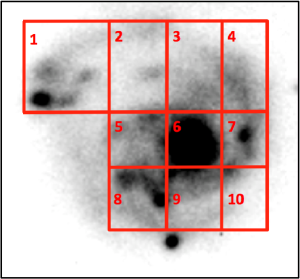
Figure 6: Full-coverage spatial binning regions for isochrone synthesis modelling, with best-fit parameters presented in Table 2

Region No.	Region	Young Comp.	Young
	Description	Age [Myr]	Comp. [%]
Region 1	Tidal Tail (V-Band)	25	30
Region 2	Tidal Tail (H$\beta$)	25, 640	30, 2
Region 3	Knotty Reg. 1	640	100
Region 4	Knotty Reg. 2	100	40
Region 5	Companion	640	100
Region 6	Extended [OIII]	900	70
Region 7	Inner Nucleus	640, 5	90, 2

Table 3: Best-fit ages and luminosity contributions of young stellar burst populations in MRC B1221$-$423, associated with morphological feature-specific binning regions in Fig. 7

Figure 7: Morphological feature-specific spatial binning regions for isochrone synthesis modelling, with best-fit parameters presented in Table 3

We repeated the fitting procedure with the more tightly defined regions in Fig. 7. This allowed us to zoom in and examine the specific morphological features identified in the V-band image. The results for this second set of regions are given in Table 3 and show that restricting the spatial extent of the fitting regions does not significantly alter the age of the fit in cases where direct comparison between the fit regions could be made.

We now discuss the models, with a particular focus on the interaction history of this system. The tidal tail region of the companion (Fig. 7, binning regions 1 and 2) is inherently dim, but the binned spectra still provide adequate signal-to-noise levels. Young populations clearly provide a superior fit to these regions, with a substantial contribution from stars dated at $\sim$25 Myr. This is not unexpected, since star formation has often been observed in the gaseous tidal tails of galaxies (e.g., Jarrett et al. 2006).

The host nucleus (Fig. 8(e)) and companion spectra show evidence for more complex underlying stellar populations than the other regions. Both show significant features that are not fully characterised by any combination of the two-component models, though several combinations provide close fits. More specifically, two-component models were unable to fit all of the main spectral features. It is likely that these regions have either seen multiple starburst episodes, or are currently undergoing a significant amount of star formation. Both of these scenarios may apply, and this is consistent with the picture of a prolonged period of interaction between the two galaxies, as we would expect if the companion galaxy has made multiple close passes. See, for example, the behaviour exhibited by the NGC 1512/1510 system (Koribalski & López-Sánchez 2009), and IRAS 08339+6517 (López-Sánchez et al. 2006).

Another feature of note is that the stellar population in the extended [O III] region described in section 3.1.1 (see also Fig. 7, region 6) shows no sign of a very young component. Given the strength of the [O III] emission from this region, this suggests that the ionization mechanism is not star formation, as discussed in section 3.1.2.

In section 3.1.1, it was suggested that one plausible cause for the fact that we see separate tidal tails in H$\beta$ emission and the V-band continuum is that these features could have been drawn out on consecutive orbits, with the first orbit producing the V-band tail, which subsequently formed stars and had the remainder of its gas stripped away. The H$\beta$ tidal tail may then have been created on the most recent encounter, with star formation just commencing. If correct, the population ages of these two features should differ by an amount approximately equal to the orbital period of the companion, estimated to be $\sim 10^{8}$ years (Johnston et al. 2010). However, we do not see any difference between the fits in the two regions: both share a significant and very young population of $\sim$25 Myr. The age of the stars in these features indicate that these features were created during the most recent close encounter, and that prodigious star formation is occurring in the tidal wake of the companion.

Finally, a potentially interesting result peculiar to the fits derived for region 6 in Fig. 8(d) is that by increasing the reddening parameter $A_{V}$ from 2.2 to 3.2, the fitting routine will fit populations as young as 5 Myr. This possible young population only constitutes a very small fraction of the SSP combination, but a component of this age would be consistent with the findings of Johnston et al. (2010), who fit a young 10 Myr population to the broadband spectral energy distribution in the host nucleus.

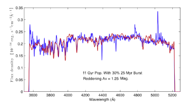
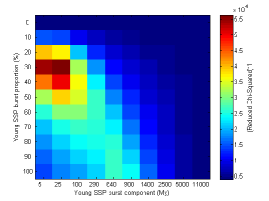
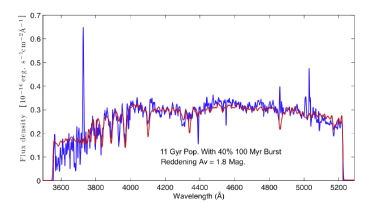
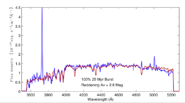
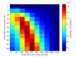
Figure 8: Model stellar population fits for selected binning regions of the MRC B1221$-$423 system shown in Fig. 6, with panels (a) & (b) above calculated from binning region #2 (tidal tail), panels (c) & (d) from binning region #8 (knotty star-burst region), and panels (e) & (f) from binning region #6 (host nucleus). The blue trace represents the actual binned data (including emission features not modelled by the SSPs), while the red trace shows the spectrum generated by the best-fitting combination of SSP models. The colour plots to the right show the inverse $\tilde{\chi}^{2}$ score for each SSP combination tried (see section 3.3.1). Higher values indicate closer fits of the model to the data.

4 Discussion and Conclusions

We have presented an IFU study of MRC B1221$-$423, a system hosting a young CSS source currently undergoing a minor merger. Our main findings are:

• strong emission from H$\beta$, [O III] and [O II] throughout the system, with spatial distributions suggestive of both AGN-like processes and extensive ongoing star formation

• diagnostic emission-line ratios indicating that AGN and star-formation processes are associated with distinct morphological features visible in broadband images

• smooth, rotation-like velocity profiles across the system in H$\beta$, with more complex kinematic behaviour observed in [O II], allowing us to develop toy models describing the interaction geometry of the host and companion galaxies

• stellar population ages derived from SSP modelling indicating the existence of distinct stellar populations of various ages occupying spatially distinct regions in the system.

The observed distribution of ionized H$\beta$ and [O II] emission throughout the system is highly suggestive of widespread ongoing star formation, while the [O III] emission appears to trace the presence of higher excitation activity associated with the AGN. Although some of the [O III] emission may be coming from highly-ionised areas within star-formation regions, some form of AGN-induced ionisation is favoured by the diagnostic line-ratio analysis in section 3.2.1. The line emission is spatially correlated with the nuclear region of the host, the companion galaxy, and blue knotty regions seen in the $V$-band optical image. These sites of active star formation suggest recent, widespread disturbance and/or injections of gas into the system. In particular, the association of this gas with what appears to be a tidal tail linking the companion and host galaxy may provide evidence of the sequence of events leading to the widespread star formation. We put forward two plausible explanations for this apparent tidal structure:

1. that the companion has dragged the gas out as it has passed through the outer envelope of the host, or

2. that the gas is being tidally stripped from the companion by the host.

In either case, structures of this type might broadly be expected in light of hierarchical merger simulations (e.g. Tissera et al. 2002). Modelling also shows that much of this gas will eventually sink into the nuclear regions of the host (e.g., Hernquist & Mihos 1995). Thus, the ample reserves of gas in this system clearly have the potential to fuel current and future AGN activity.

The kinematic behaviour of the gas in the system was examined via the radial velocities of each of the major lines within our spectral coverage. On the broadest spatial scales, the data show a smooth rotation of the system inclined to our line of sight. There is an ambiguity in the orbital geometry of the system that we were unable to resolve. We have, however, been able to use the data to arrive at two possible toy models for the geometry of the interaction, illustrated in Figure 5. These models provide a basic geometrical picture of the merger event, are able to account for the basic morphological and kinematic structures, including the tidal shells visible in V-band images, the structure of the tidal tail joining companion and host, and the streams of gas apparent in our kinematic analysis. The higher-excitation oxygen lines reveal a more complex kinematic picture than that revealed in H$\beta$, particularly in the nuclear regions. The nature of this complexity might perhaps shed further light on the dynamics of the interaction, but this will require detailed modelling beyond the scope of the current work. Overall, the rotational kinematics are consistent with a minor merger interaction, first posited for this system by Safouris et al. (2003), and built upon by Johnston et al. (2005, 2010).

Our isochrone synthesis modelling in section 3.3 shows evidence for stellar populations of different ages inhabiting spatially distinct regions of the host and companion. We find that population ages throughout the system cluster about specific values, particularly 100 Myr and 640 Myr, albeit with coarse temporal resolution. There is some evidence hinting at a young population of 5 Myr in the nuclear region of the host, but higher spatial resolution will be required to confirm this. The ages derived in our study differ from some of those obtained by Johnston et al. (2005, 2010). However, given the significant differences in spectral and spatial coverage between the two techniques, this is perhaps not surprising.

Metallicities derived across the MRC B1221$-$423 system are similar for most regions (see Table  1). However, the fact that the metallicity for the companion is marginally the lowest (notwithstanding the 0.1–0.2 dex errors typical of the method used), followed by that for the region containing the significant 100 Myr-old stellar population, is consistent with the ages and sequence of events we propose below.

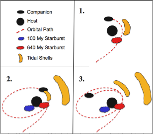
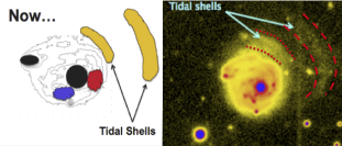
Figure 9: Proposed sequence of events in the triggering of MRC B1221$-$423, based on results described here, and by Johnston et al. (2010), Johnston et al. (2005), and Safouris et al. (2003). The widespread ongoing star formation, the prominent starburst populations at 640 Myr and 100 Myr, the two shells of tidally disrupted material visible in broadband images, the tidal tail being pulled out by the companion and the recently triggered CSS source are all consistent with the sequence of events associated with the minor merger scenario proposed in this figure.

Given the data accumulated for this system from photometry, spectroscopy and radio imaging, we now present a possible timeline and sequence of events leading from the initial interaction of the two galaxies through to the present epoch. The approximate orbital period of the companion was estimated by Johnston et al. (2010) to be $\sim 10^{8}$ years. We now suggest that this estimate may be too low. If the companion was initially captured into a highly eccentric orbit of period $\sim$3-5$\times 10^{8}$ years, bursts of intense star formation (identified by our stellar population modelling) may have been triggered by consecutive strong interactions near the periapses of the companion’s orbit. On this basis, we propose the following sequence of events, depicted schematically in Figure 9:

1) The companion makes an initial close pass by the host galaxy, interacting strongly with it. Gas is either stripped from the companion by the host, or gas already within the host is dynamically disturbed. In either case, it subsequently begins forming stars—the 640 Myr-old starburst. Some gas also begins to sink down into the nuclear region of the host. A shell of stars is thrown out of the host, the companion loses orbital energy, and becomes trapped into an eccentric orbit.

2) The companion then moves out on its orbit to apogalacticon and then back to perigalacticon once again, taking somewhere on the order of $\sim$3$\times 10^{8}$ years. The ensuing interaction triggers a second major episode of gas stripping/star formation—the 100 Myr-old starburst—and throws out a second shell of stars. The tidal tail visible in optical images begins to be pulled out of the host or companion at this stage. Some of the stripped gas sinks to the core of the host galaxy, fuelling the supermassive black hole and triggering the radio-loud AGN.

3) We find the system in its current state about 100 Myr after this latest perigalacticon, and can compare it to the false-colour optical image in Figure 9. We can identify the two shells of stars pulled out of the system, and stellar populations resulting from star bursts corresponding to the periods of most intense interaction approximately 100 Myr and 640 Myr ago. The CSS radio source has recently been switched on, after the gas has had $\sim$100 Myr to sink into the nuclear regions, in approximate agreement with the timescales over which such processes are thought to occur (e.g., Lin, Pringle & Rees 1988). Johnston et al. (2010) show that the CSS source is potentially undergoing a dramatic interaction with a dense surrounding environment — the gas stripped from the companion that has been drawn towards the nucleus of the host galaxy.

Projecting into the future, the companion is expected to continue to lose orbital energy and merge fully with the host.

References

- Ballantyne et al. (2006) Ballantyne, D. R., Everett, J. E., & Murray, N. 2006a, ApJ, 639, 740
- Barai et al. (2011) Barai, P., Martel, H., & Germain, J. 2011, ApJ, 727, 54
- Barnes & Hernquist (1991) Barnes, J.E. & Hernquist, L. 1991, ApJ, 370, L65
- Best et al. (1996) Best, P. N., Longair, M. S., & Röttgering, H. J. A. 1996, MNRAS, 280, L9
- Bruzual & Charlot (2003) Bruzual, G. & Charlot, S. 2003, MNRAS, 344, 1000
- Calzetti (2000) Calzetti, D. et al, 2000, ApJ, 533, 682
- Calzetti (2007) Calzetti, D. et al, 2007, ApJ, 666, 870
- Cisternas et al. (2011) Cisternas, M., Jahnke, K., & Inskip, K. J. et al. 2011, ApJ, 726, 57
- Croom (2012) Croom, S.M. et al., 2012, MNRAS, 421, 872
- Di Matteo et al. (2005) Di Matteo, T., Springel, V., & Hernquist, L. 2005, Nature, 433, 604
- Fabian (1999) Fabian, A.C., 1999, MNRAS, 308, L39
- Ferrarese & Merritt (2000) Ferrarese, L., & Merritt, D. 2000, ApJ, 539, L9
- Gabor et al. (2009) Gabor, J. M., et al. 2009, ApJ, 691, 705
- Gebhardt (2000) Gebhardt, K. et al. 2000, ApJ, 539, L13
- Germain et al. (2009) Germain, J., Barai, P., & Martel, H. 2009, ApJ, 704, 1002
- Ginzburg & Syrovatskii (1965) Ginzburg, V.L., Syrovatskii, S.I. (1965): Ann. Rev. A. & A. 3, 297
- Grogin et al. (2005) Grogin, N. A., et al. 2005, ApJ, 627, L97
- Hasinger (2008) Hasinger, G. 2008, A&A, 490, 905
- Hernquist & Mihos (1995) Hernquist, L., & Mihos, J. C. 1995, ApJ, 448, 41
- Hillas (1984) Hillas, A. M., ARAA, 22, 425 (1984)
- Hopkins & Hernquist (2009) Hopkins, P. F. & Hernquist, L. 2009, ApJ, 694, 599
- Jafelice et al. (1992) Jafelice, L. C., & Opher, R. 1992, MNRAS, 257, 135
- Jarrett et al. (2006) Jarrett T. et al., 2006, AJ, 131, 261
- Johnston et al. (2010) Johnston, H. M., Broderick, J. W., Cotter, G., Morganti, R. & Hunstead, R. W., 2010, MNRAS, 407, 721
- Johnston et al. (2005) Johnston, H. M., Hunstead R. W., Cotter G., Sadler E. M., 2005, MNRAS, 356, 515
- King (2003) King, A. 2003, ApJ, 596, L27
- Kobulnicky & Kewley (2004) Kobulnicky H. A., Kewley L. J., 2004, ApJ, 617, 240
- Koss et al. (2010) Koss, M., Mushotzky, R., Veilleux, S., & Winter, L. 2010, ApJ, 716, L125
- Koribalski, B.S. & Lopez-Sanchez (2009) Koribalski, B.S. & López-Sánchez, Á.R., 2009, MNRAS, 400, 1749
- Kronberg et al. (2001) Kronberg, P. P., Dufton, Q. W., Li, H., & Colgate, S. A. 2001, ApJ, 560, 178
- Lamareille (2010) Lamareille F., 2010, A&A, 509, A53
- Le Fèvre et al. (2003) LeFèvre O. et al., 2003, in Iye M., Moorwood A. F. M., eds, SPIE, Volume 4841, Commissioning and performances of the VLT-VIMOS instrument, p. 1670
- Li et al. (2006) Li, C., Kauffmann, G., Wang, L., White, S. D. M., Heckman, T. M., & Jing, Y. P. 2006, MNRAS, 373, 457
- Lin et al. (1988) Lin, D.N.C., Pringle, J.E. & Rees, M.J. 1988. Ap. J. 328:103
- Longair et al. (1995) Longair, M. S., Best, P. N., & Röttgering, H. J. A. 1995, MNRAS, 275, L47
- Lopez-Sanchez et al. (2006) López-Sánchez, Á.R., Esteban, C. & Garcia-Rojas, J., 2006, A&A, 448, 997
- Lopez-Sanchez et al. (2010) López-Sánchez, Á.R., 2010 A&A, 521, 63
- Lopez-Sanchez et al. (2010b) López-Sánchez, Á.R., Esteban, C.,2010 A&A, 517, 85
- Lotz et al. (2011) Lotz J. M., Jonsson P., Cox T. J., Croton D., Primack J. R., Somerville R. S., Stewart K., 2011, ApJ, 742, 103
- Lutz et al. (2010) Lutz, D., Mainieri, V., & Rafferty, D. et al. 2010, ApJ, 712, 1287
- Mezcua et al. (2012) Mezcua, M., Chavushyan, V. H., Lobanov, A. P. & León-Tavares, J. 2012, A&A, 544, 36
- Mihos & Hernquist (1996) Mihos, J.C. & Hernquist, L. 1996, ApJ, 464, 641
- Miller et al. (2003) Miller, C. J., Nichol, R. C., Gomez, P. L., Hopkins, A. M., & Bernardi, M. 2003, ApJ, 597, 142
- O’Dea (1998) O’Dea, C. P., 1998, PASP, 110, 493
- Pérez-Montero (2002) Pérez-Montero E., 2002, PhD thesis, Universidad Autónoma de Madrid
- Press et al. (2007) Press, W.H., Teukolsky, S.A., Vetterling, W.T., Flannery, B.P. 2007. Numerical Recipes: The Art of Scientific Computing, Third Edition : Cambridge University Press.
- Safouris et al. (2003) Safouris V., Hunstead R. W., Prouton O. R., 2003, Proc. Astron. Soc. Aust., 20, 1
- Salpeter (1955) Salpeter, E. E. 1955, ApJ, 121, 161
- Sánchez et al. (2012) Sánchez, S.F. et al., 2012, A&A, 538, A8
- Sanders et al. (1996) Sanders, D. B., & Mirabel, I. F. 1996, ARA&A, 34, 749
- Sanders et al. (1988) Sanders, D. B., et al. 1988a, ApJ, 325, 74
- Schlegel et al. (1998) Schlegel D. J., Finkbeiner D. P., Davis M., 1998, ApJ, 500, 525
- Scodeggio et al. (2005) Scodeggio, M., et al. 2005, PASP, 117, 1284
- Silk & Rees (1998) Silk, J., & Rees, M. J. 1998, A&A, 331, L1
- Simpson et al. (1993) Simpson, C., Clements, D. L., Rawlings, S., & Ward, M. 1993 MNRAS, 262, 889
- Stewart (2009) Stewart, K. R. 2009, Galaxy Evolution: Emerging Insights and Future Challenges (ASP Conf. Ser. 419), ed. S. Jogee, I. Marinova, L. Hao, & G. A. Blanc (San Francisco, CA: ASP), 243
- Taniguchi et al. (1999) Taniguchi, Y. 1999, ApJ, 524, 65
- Tissera et al. (2002) Tissera P. B., Dom nguez-Tenreiro R., Scannapieco C., S iz A., 2002, MNRAS, 333, 327
- Veilleux (2001) Veilleux, S. 2001, in Starburst Galaxies: Near and Far, ed. L. Tacconi & D. Lutz (Heidelberg: Springer), 88-95
- Zaritsky (1997) Zaritsky, D., Smith, R., Frenk, C., & White, S. D. M. 1997, ApJ, 478, 39