Gaussian beam methods for the Helmholtz equation

Abstract.

In this work we construct Gaussian beam approximations to solutions of the high frequency Helmholtz equation with a localized source. Under the assumption of non-trapping rays we show error estimates between the exact outgoing solution and Gaussian beams in terms of the wave number $k$, both for single beams and superposition of beams. The main result is that the relative local $L^{2}$ error in the beam approximations decay as $k^{-N/2}$ independent of dimension and presence of caustics, for $N$-th order beams.

1. Introduction

In this article we are interested in the accuracy of Gaussian beam approximations to solutions of the high frequency Helmholtz equation with a source term,

(1) $$L_{n}u=_{def}\Delta u+(i\alpha k+k^{2})n^{2}u=f,\qquad x\in\mathbb{R}^{d}.$$

Here $k>0$ is the wave number, assumed to be large, $n(x)$ is the index of refraction and $f(x;k)$ is a source function which in general also depends on $k$. We assume that both $f(x;k)$ and $n(x)-1$ vanish for $|x|>R$. The nonnegative parameter $\alpha$ represents absorption. It is zero in the limit of zero absorption, where $L^{2}$ solutions of (1) become solutions satisfying the standard radiation condition.

The Helmholtz equation (1) is widely used to model wave propagation problems in application areas like electromagnetics, geophysics and acoustics. Numerical simulation of Helmholtz becomes expensive when the frequency of the waves is high. In direct discretization methods a large number of grid points is then needed to resolve the wave oscillations, and the computational cost to maintain constant accuracy grows algebraically with the frequency. The Helmholtz equation is typically even more difficult to handle in this regime than time-dependent wave equations, as numerical discretizations lead to large indefinite and ill-conditioned linear systems of equations, for which it is difficult to find efficient preconditioners [12]. At sufficiently high frequencies direct simulations are not feasible.

As an alternative one can use high frequency asymptotic models for wave propagation, such as geometrical optics [29, 11, 44], which is obtained when the frequency tends to infinity. The solution of the partial differential equation (PDE) is assumed to be of the form

(2) $$u=ae^{ik\phi},$$

where $\phi$ is the phase, and $a$ is the amplitude of the solution. In the limit $k\to\infty$ the phase and amplitude are independent of the frequency and vary on a much coarser scale than the full wave solution. They can therefore be computed at a computational cost independent of the frequency. However, a main drawback of geometrical optics is that the model breaks down at caustics, where rays concentrate and the predicted amplitude $a$ becomes unbounded.

Gaussian beams form another high frequency asymptotic model which is closely related to geometrical optics. However, unlike geometrical optics, the phase $\phi$ is complex-valued, and there is no breakdown at caustics. The solution is still assumed to be of the form (2), but it is concentrated near a single ray of geometrical optics. To form such a solution, we first pick a ray and solve systems of ordinary differential equations along it to find the Taylor expansions of the phase and amplitude in variables transverse to the ray. Although the phase function is real-valued along the central ray, its imaginary part is chosen so that the solution decays exponentially away from the central ray, maintaining a Gaussian-shaped profile. For the simplest first order beams the phase $\phi$ is a second order Taylor expansion, while the amplitude $a$ is a zeroth order expansion. For wave equations one can use time as a parameter for the rays, and the expressions for the phase and amplitude are

(3) $$\phi(t,y)=\phi_{0}(t)+(y-x(t))\cdot p(t)+\frac{1}{2}(y-x(t))\cdot M(t)(y-x(t)),\qquad a(t,y)=a_{0}(t)$$

where $x(t)$ is the geometrical optics ray, $p(t)$ is the direction of the ray and the second derivative matrix $M(t)$ encodes the width and curvature of the beam; $M$ has a positive definite imaginary part which ensures the beam has a Gaussian shape. In the Helmholtz case, since there is no longer a distinguished variable with level sets transverse to the rays, one uses Taylor expansion in the plane orthogonal to the ray direction. Higher order beams are constructed through higher order Taylor expansions in (3).

The existence of Gaussian beam solutions to the wave equation has been known since sometime in the 1960’s, first in connection with lasers, see Babič and Buldyrev [2]. Later, they were used in the analysis of propagation of singularities in PDEs by Hörmander [21] and Ralston [39]. In the context of the Schrödinger equation first order beams correspond to classical coherent states. Higher order versions of these have been introduced to approximate the Schrödinger equation in quantum chemistry by e.g. Heller [16], Hagedorn [14], Herman and Kluk [17].

More general high frequency solutions that are not necessarily concentrated on a single ray can be described by superpositions of Gaussian beams. This idea was first introduced by Babič and Pankratova in [3] and was later proposed as a method for approximating wave propagation by Popov in [41]. Letting the beam parameters depend on their initial location $z$, such that $x=x(t;z)$, $p=p(t;z)$ etc., and $a=a(t,y;z)$, $\phi=\phi(t,y;z)$, the approximate solution for an initial value problem can be expressed with the superposition integral

(4) $$u(t,y)=\left(\frac{k}{2\pi}\right)^{\frac{d}{2}}\int_{K_{0}}a(t,y;z)e^{ik\phi(t,y;z)}dz\ ,$$

where $K_{0}$ is a compact subset of ${\mathbb{R}}^{d}$.

It should be mentioned that there are other related Gaussian beam like approximations. In the thawed Gaussian approximation [15] the phase $\phi$ is always a second order polynomial. Higher order is obtained by instead taking a higher order polynomial in the amplitude, to correct also for errors in the phase. Frozen Gaussian approximations [16, 17] also use a second order polynomial for the phase $\phi$, but with a fixed size of the second derivative ($M(t)$=constant). Single frozen Gaussians are therefore not asymptotic solutions to the wave equation. However, superpositions of frozen Gaussians are and they can be thought of as an efficient linear basis for the wave equation.

Numerical methods based on Gaussian beam superpositions go back to the 1980’s with work by Popov, [41, 27], Cerveny [10] and Klimeš [30] for high frequency waves and e.g. Heller, Herman, Kluk [16, 17] in quantum chemistry. In the past decade there was a renewed interest in such methods for waves following their successful use in seismic imaging and oil exploration by Hill [18, 19]. Development of new beam based methods are now the subject of intense interest in the numerical analysis community and the methods are being applied in a host of applications, from the original geophysical applications to gravity waves [46], the semiclassical Schrödinger equation [13, 24, 31], and acoustic waves [45]. See also the survey of Gaussian beam methods in [23]. Individual beams are normally computed in a Lagrangian fashion by solving ODEs along the central rays. The superposition is then replaced by a discrete summation of beams. There are also more recent numerical techniques based on Eulerian formulations of the problem [32, 24, 25, 31, 42]. In these methods a PDE is derived for the parameters in the beams, i.e. the quantities in the ODEs. This is coupled with a level-set PDE for the ray dynamics. With the Eulerian formulation the result is no longer a superposition of asymptotic solutions to the wave equation! For superpositions over subdomains moving with the Hamiltonian flow, it was shown directly in [34, 35] that they are asymptotic solutions without reference to standard Gaussian beams. Numerical approaches for treating general high frequency initial data for superposition over physical space were considered in [47, 1] for the wave equation.

In this paper we study the accuracy in terms of $k$ of Gaussian beams and superpositions of Gaussian beams for the Helmholtz equation (1). This would give a rigorous foundation for beam based numerical methods used to solve the Helmholtz equation in the high frequency regime. In the time-dependent case several such error estimates have been derived in recent years: for the initial data [45], for scalar hyperbolic equations and the Schrödinger equation [34, 35, 36], for frozen Gaussians [43, 33] and for the acoustic wave equation with superpositions in phase space [7]. The general result is that the error between the exact solution and the Gaussian beam approximation decays as $k^{-N/2}$ for $N$-th order beams in the appropriate Sobolev norm. There are, however, no rigorous error estimates of this type available for the Helmholtz equation. What is known is how well the beams asymptotically satisfy the equation, i.e. the size of $L_{n}u$ for a single beam. Let us also mention an estimate of the Taylor expansion error away from caustics, [38].

The analysis of Gaussian beam superpositions for Helmholtz presents a few new challenges compared to the time-dependent case. First, it must be clarified precisely how beams are generated by the source function and how the Gaussian beam approximation is extended to infinity. This is done in §2 and §3 for a compactly supported source function that concentrates on a co-dimension one manifold. Second, additional assumptions on the index of refraction $n(x)$ are needed to get a well-posed problem with $k$-independent solution estimates and a well-behaved Gaussian beam approximation at infinity. The conditions we use are that $n(x)$ is non-trapping and that there is an $R$ for which $n(x)$ is constant when $|x|>R$.

In §4 we consider the difference between the Gaussian beam approximation and the exact solution to the radiation problem with the corresponding source function. Here we are interested in behavior of the local $L^{2}$ norm $||u_{GB}-u||_{L^{2}(|x|<R)}$ as $k\to\infty$. This depends on the well-posedness of the radiation problem. There are a variety of estimates that apply here [40, 8], but the Laplace-transform based estimates of Vainberg [48, 49] suffice for our purposes. In §5 we compare the Gaussian beam approximation with the result of stationary phase expansion of the exact solution in a simple example.

Sections §6 and §7 are devoted to superpositions of beams with fundamental source terms. Our main result is Theorem 6.1 where we are able to show that the error between superposition of $N$-th order beams and the exact outgoing solution decays as $k^{-N/2}$ independent of dimension and presence of caustics. This is consistent with the optimal results of [36] in the time-dependent setting. Finally, §7 gives an example of how beams can be constructed for more general source functions.

2. Construction of Gaussian beams

In this section we construct the Gaussian beam solutions for (1) when $f$ is compactly supported on a co-dimension one manifold. This construction has become standard (see, for example, [39] or [28]) and we review some details here which will be used later. The form of the beam solutions is

(5) $$u(x;k)=e^{ik\phi(x)}(a_{0}(x)+a_{1}(x)k^{-1}+\cdots+a_{\ell}(x)k^{-\ell}).$$

Each beam concentrates on a geometrical optics ray $\gamma=\{x(s):s\in\mathbb{R}\}$, which is the spatial part of the bicharacteristics $(x(s),p(s))$ defined by the flow for the Hamiltonian $H(x,p)=|p|^{2}-n^{2}(x)$

(6) $$\dot{x}=2p,\quad\dot{p}=-\nabla_{x}n^{2}(x).$$

We assume that there is a number $R>0$ such that the (smooth) index of refraction satisfies $n(x)\equiv 1$ when $|x|>R$ and that the source function $f$ is compactly supported in $\{|x|<R\}$. Here we also restrict the construction of the Gaussian beam solution to the larger region $|x|\leq 6R$. The essential additional hypothesis for our construction is that the index of refraction does not lead to trapped rays. The precise non-trapping condition is that there is an $L$ such that $|x(L)|>2R$ for all solutions with $|x(0)|<R$ and $H(x(0),p(0))=0$. Note that this implies that $|x(s)|>2R$ for $s>L$ since rays are straight lines when $n(x)\equiv 1$.

Applying $L_{n}$ in (1) to (5) we have

(7) $$L_{n}u=e^{ik\phi}\sum_{j=-2}^{\ell}c_{j}(x)k^{-j},$$

where

$$c_{-2} =(n^{2}-|\nabla_{x}\phi|^{2})a_{0}=_{def}E(x)a_{0},$$

$$c_{-1} =i\alpha n^{2}a_{0}+\nabla_{x}\cdot(a_{0}\nabla_{x}\phi)+\nabla_{x}a_{0}\cdot\nabla_{x}\phi+Ea_{1},$$

$$c_{j} =i\alpha n^{2}a_{j+1}+\nabla_{x}\cdot(a_{j+1}\nabla_{x}\phi)+\nabla_{x}a_{j+1}\cdot\nabla_{x}\phi+Ea_{j+1}+\Delta_{x}a_{j},\quad\ j=0,1,\ldots,\ell.$$

ODEs for $S(s)=\phi(x(s))$, $M(s)=D^{2}\phi(x(s))$ and $A_{0}(s)=a_{0}(x(s))$ arise from requiring that $c_{-2}$ vanishes to third order on the ray $x(s)$, and that $c_{-1}$ vanishes to first order on the ray. It leads to the equations

(8) $$\dot{S}=2n^{2}(x(s))\qquad\dot{M}=D^{2}(n^{2})(x(s))-2M^{2}\qquad\dot{A}_{0}=-{\rm tr}(M(s))A_{0}-\alpha n^{2}(x(s))A_{0}.$$

This amounts to constructing a “first order” beam. Higher order beams can be constructed by requiring $c_{-2}$ vanishes to higher order on $\gamma$. Then one can require that the $c_{j}$’s with $j>-2$ also vanish to higher order, and obtain a recursive set of linear equations for the partial derivatives of $a_{0},a_{1},\ldots,a_{\ell}$. More precisely, for an $N$-th order beam $\ell=\lceil N/2\rceil-1$ in (5) and $c_{j}(x)$ should vanish to order $N-2j-2$ when $-2\leq j\leq\ell-1$.

For initial data, we let $S(0)=0$ and choose $M(0)$ so that

(9) $$M(0)=M(0)^{\top},\qquad M(0)\dot{x}(0)=\dot{p}(0),\qquad\text{${\rm Im}\{M(0)\}$ is positive definite on $\dot{x}(0)^{\perp}$}.$$

Then for all $s$ the matrix $M(s)$ inherits the properties of $M(0)$: $M(s)\dot{x}(s)=\dot{p}(s)$, $M(s)=M(s)^{\top}$, and ${\rm Im}\{M(s)\}$ is positive definite on the orthogonal complement of $\dot{x}(s)$, see [39]. For the amplitude we take $A_{0}(0)=1$. We can solve the ODE for $A_{0}$ explicitly, and obtain

$$A_{0}(s)=\exp\left(-\int_{0}^{s}(\alpha n^{2}(x(\tau))+{\rm tr}(M))d\tau\right).$$

The phase $\phi$ in (5) can be any function satisfying $\phi(x(s))=S(s)$, $\nabla\phi(x(s))=p(s)$ and $D^{2}\phi(x(s))=M(s)$. However, to write down such a function we need to have $s$ as a function of $x$. Since we have $\dot{x}(s)\neq 0$, $x(s)$ traces a smooth curve $\gamma$ in $\mathbb{R}^{d}$, and the non-trapping hypothesis implies that this curve is a straight line when $|s|>L$. We let

$$\Omega(\eta)=\{x\,:\,|x|\leq 6R\ \text{\rm and}\ |x-\gamma|\leq\eta\},$$

be the tubular neighborhood of $\gamma$ with radius $\eta$ in the ball $\{|x|\leq 6R\}$. By choosing $\eta$ small enough, we can uniquely define $s=s(x)$ for all $x\in\Omega(\eta)$ such that $x(s)$ is the closest point on $\gamma$ to $x$, provided $\gamma$ has no self-intersections. We then define the phase function $\phi$ and amplitude $A$ on $\Omega$ for first order beams by

(10) $$\phi(x)=S(s)+p(s)\cdot(x-x(s))+\frac{1}{2}(x-x(s))\cdot M(s)(x-x(s)),\qquad A(x)=A_{0}(s),$$

with $s=s(x)$. Note that $s(x)$ is constant on planes orthogonal to $\gamma$ intersected with $\Omega(\eta)$. Since $\gamma$ can have only finitely many self-intersections, we can cut $\gamma$ into segments without self-intersections, and define $s(x)$ on a tubular neighborhood each segment, ignoring the endpoints. For this reason self-intersections will not create difficulties, and without loss of generality we will assume that $\gamma$ has no self-intersections in what follows. The construction of the Gaussian beam phase and amplitude for higher order beams is carried out in a similar way [39].

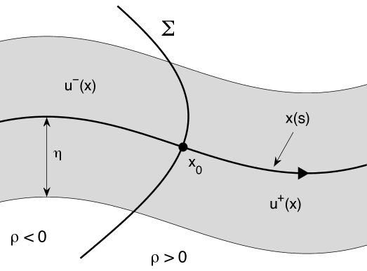
Figure 1. Notation for the source in two dimensions. The gray area indicates $\Omega(\eta)$.

2.1. Source

To introduce the source functions that we will consider in this article let $\rho$ be a function such that $|\nabla\rho|=1$ on $\{x:\rho(x)=0\}$, and define $\Sigma$ to be the hypersurface $\{x:\rho(x)=0\}$. Given $x_{0}\in\Sigma$, we let $(x(s),p(s))$ be the solution of (6) with $(x(0),p(0))=(x_{0},n(x_{0})\nabla\rho(x_{0}))$. Since we assume no trapped rays and $n(x)\equiv 1$ when $|x|>R$, $x(s)$ and $p(s)$ are defined for $s\in\mathbb{R}$, and we set $\gamma=\{x(s),s\in\mathbb{R}\}$. Then we can assume that $s(x)$ is defined on the tubular neighborhood $\Omega(\eta)$ of $\gamma$ as above (assuming no self-intersections). We begin with a beam $u(x,k)$ concentrated on $\gamma$, and defined on $\Omega(\eta)$. If $u$ is first order, we can define it by (10). Then we define $u^{+}$ to be the restriction of $u$ to $\{x:\rho(x)\geq 0\}$. In order to have a source term which is a multiple of $\delta(\rho)$, we need a second beam $u^{-}(x,k)$ defined on $\{x:\rho(x)\leq 0\}$ which is equal to $u^{+}$ on $\Sigma$ for all $k$. Hence, writing $u^{+}(x,k)=A^{+}(x,k)e^{ik\phi^{+}(x)}$ and $u^{-}(x,k)=A^{-}(x,k)e^{ik\phi^{-}(x)}$, we must have $\phi^{+}=\phi^{-}$ and $A^{+}=A^{-}$ on $\Sigma$. Those requirements and $c_{j}=0,\ j=-2,\ldots,\ell$ at $x_{0}$ determine the Taylor series in the transverse variables at $x_{0}$ for $\phi^{-}$ and $A^{-}$. To see this suppose that $u^{-}$ is going to be a beam of order $N$ and that the coordinates on $\Omega(\eta)$ are given by $(s,y)$ where $s=s(x)$ and $y=(y_{1},\ldots,y_{d-1})$ is transversal. Then, provided $\eta$ is chosen small enough, $\Sigma$ is given by $s=\sigma(y)$ with $\sigma(0)=0$ and $\nabla\sigma(0)=0$. To determine the Taylor series in $y$ for $\phi^{-}(s,y)$ at $s=0$ one differentiates the equation $\phi^{-}(\sigma(y),y)=\phi^{+}(\sigma(y),y)$ with respect to $y$ and evaluates at $y=0$. When partial derivatives of $\phi^{-}$ with respect to $s$ appear in this calculation, they are determined by the requirement that $c_{-2}$ vanishes on $x(s)$ to order $N+2$. The Taylor series for $A^{-}$ in the transverse variables at $x_{0}$ is determined in the same way from $A^{-}(\sigma(y),y,k)=A^{+}(\sigma(y),y,k)$ for all $k$. To construct $u^{-}$, we use those Taylor series as data at $s=0$ in solving the equations $c_{j}=0,\ j=-2,\ldots,\ell$ along $x(s)$. Since for an $N$-th order beam we only require that $c_{j}$ vanishes on $x(s)$ to order $N-2j-2$, we can still require that $\phi^{+}=\phi^{-}$ and $A^{+}=A^{-}$ exactly at points on $\Sigma$. Extending $u^{+}$ to be zero in $\{x:\rho(x)<0\}$ and $u^{-}$ to be zero in $\{x:\rho(x)>0\}$, we define $u_{GB}=u^{+}+u^{-}$. Then we have, setting $A=A^{+}=A^{-}$ on $\Sigma$,

(11) $$L_{n}u_{GB} =\left[ik\left({\partial\phi^{+}\over\partial\nu}-{\partial\phi^{-}\over\partial\nu}\right)A+{\partial A^{+}\over\partial\nu}-{\partial A^{-}\over\partial\nu}\right]e^{ik\phi^{+}}\delta(\rho)+f_{GB}=_{def}g_{0}\delta(\rho)+f_{GB},$$

where $\nu(x)=\nabla\rho(x)$, the unit normal to $\Sigma$. We consider the singular part of $L_{n}u_{GB}$ in (11), i.e. $g_{0}\delta(\rho)$, to be the source term and $f_{GB}$ to be the error from the Gaussian beam construction. Note that

(12) $$f_{GB}=e^{ik\phi^{+}(x)}\sum_{j=-2}^{\ell}c^{+}_{j}(x)k^{-j}+e^{ik\phi^{-}(x)}\sum_{j=-2}^{\ell}c^{-}_{j}(x)k^{-j},$$

where the $c_{j}^{+}(x)$ are extended to be zero when $\rho(x)<0$ and the $c_{j}^{-}(x)$ are extended to be zero when $\rho(x)>0$. For first order beams $\ell=0$ and (8) implies $c^{\pm}_{-2}(x)$ and $c^{\pm}_{-1}(x)$ are $O(|x-x(s(x))|^{3})$ and $O(|x-x(s(x))|)$ respectively. Finally we restrict the support of $u_{GB}$ to $\Omega(\eta)$ by multiplying it by a smooth cutoff function supported in $\Omega(\eta)$ which is identically one on the smaller neighborhood $\Omega(\eta/2)$. The cutoff function modifies $A^{\pm}$, and $f_{GB}$, outside $\Omega(\eta/2)$, but its contribution to (11) is exponentially small in $k$ (see [36]), and we will disregard it from here on.

2.2. Estimate of $f_{GB}$

From the non-trapping condition, it follows that the length of a ray inside $\Omega(\eta)$ is bounded independently of starting point in $|x|\leq R$. By construction, $c_{\ell}^{\pm}(x)$ is bounded and

(13) $$c^{\pm}_{j}(x)=\sum_{|\beta|=N-2j-2}d^{\pm}_{\beta,j}(x)(x-x(s))^{\beta},\qquad j=-2,\ldots,\ell-1,$$

where $d^{\pm}_{\beta,j}(x)$ are bounded on $\Omega(\eta)$. Hence,

$$|c^{\pm}_{j}(x)|\leq C_{j}|x-x(s)|^{N-2j-2},\qquad x\in{\Omega(\eta)}.$$

Choosing $\eta$ sufficiently small, the construction also ensures that

(14) $${\rm Im}\{\phi^{\pm}\}(x)\geq c|x-x(s)|^{2},\qquad x\in{\Omega(\eta)},$$

see [36]. From the bound

(15) $$s^{p}e^{-as^{2}}\leq C_{p}a^{-p/2}e^{-as^{2}/2},\qquad C_{p}=(p/e)^{p/2},$$

with $p=N-2j-2$, $a=kc$ and $s=|x-x(s)|$ we then get for $x\in{\Omega(\eta)}$,

$$|f_{GB}(x)| \leq e^{-k{\rm Im}\{\phi^{\pm}\}(x)}\sum_{j=-2}^{\ell}|c^{\pm}_{j}(x)|k^{-j}\leq e^{-kc|x-x(s)|^{2}}\sum_{j=-2}^{\ell}C_{j}|x-x(s)|^{N-2j-2}k^{-j}$$

(16) $$\leq Ce^{-k{c}|x-x(s)|^{2}/2}\sum_{j=-2}^{\ell}k^{-N/2+j+1}k^{-j}\leq Ce^{-kc|x-x(s)|^{2}/2}k^{-N/2+1}.$$

We note that the constant is uniform in $|x|\leq 6R$ and in particular for first order beams $f_{GB}$ will be $O(k^{1/2}e^{-k\tilde{c}|x-x(s)|^{2}})$.

3. Extension of Gaussian beam solutions to infinity

In this section we extend $u_{GB}(x)$ defined on $|x|\leq 6R$ to an outgoing solution $\tilde{u}_{GB}(x)$ in $\mathbb{R}^{d}$. For estimates on the validity of the approximation it is essential to do this so that

$${\tilde{f}_{GB}=_{def}L_{n}\tilde{u}_{GB}-g_{0}\delta(\rho)},$$

is supported in $|x|<6R$ and is $o(k)$.

The main step in the extension is a simplified version of the procedure used in [37]. Let $G_{\lambda}(x)$ be the Green’s function for the Helmholtz operator $\Delta+\lambda^{2}$, where $\lambda$ may be complex valued. When $\alpha\geq 0$, define

(17) $$k_{\alpha}:=\sqrt{k^{2}+ik\alpha}.$$

Then $L_{1}=\Delta+i\alpha k+k^{2}=\Delta+k_{\alpha}^{2}$, and $G_{k_{\alpha}}$ is uniquely determined when $\alpha>0$ as the inverse of the self-adjoint operator $L_{1}$; for $\alpha=0$ it can be defined either as $\lim_{\alpha\downarrow 0}G_{k_{\alpha}}$ or by radiation conditions. In the case $d=3$,

$$G_{{k_{\alpha}}}(x)=-(4\pi)^{-1}\left(\frac{e^{ik_{\alpha}|x|}}{|x|}\right).$$

To extend $u_{GB}$ we introduce the cutoff function $\eta_{a}(x)$ in $C^{\infty}(\mathbb{R}^{d})$ with parameter $a\geq 1$:

$$\eta_{a}(x)=\left\{\begin{array}[]{ll}1&|x|<(a-1)R\\ 0&|x|>aR\end{array}\right.$$

(see Figure 2) and define

Figure 2. The cut off functions $\eta_{3}(x)$ and $\eta_{5}(x)$.

(18) $$\tilde{u}_{GB}=\eta_{3}(x)u_{GB}(x)+\int G_{{k_{\alpha}}}(x-y)\eta_{5}(y)L_{n}[(1-\eta_{3}(y))u_{GB}(y)]dy.$$

We also assume that $R$ is chosen large enough such that the support of $g_{0}\delta(\rho)\subset\Sigma\cap{\Omega(\eta)}$ is inside $\{|x|<R\}$.

Consider first $L_{n}\tilde{u}_{GB}$ in the region $\{|x|\geq R\}$. Since $L_{n}=L_{1}$ as well as $g_{0}\delta(\rho)=0$ in this region and $\eta_{5}\equiv 1$ on the support of $\eta_{3}$,

$${\tilde{f}_{GB}(x)} =L_{n}\tilde{u}_{GB}(x)=\eta_{5}(x)L_{n}[\eta_{3}(x)u_{GB}(x)]+\eta_{5}(x)L_{n}[(1-\eta_{3}(x))u_{GB}(x)]$$

$$=\eta_{5}(x)L_{n}u_{GB}{=\eta_{5}(x){f}_{GB}(x)}.$$

Since $\eta_{5}$ is supported on $|x|<5R$, it follows that $\tilde{f}_{GB}$ vanishes for $|x|>5R$.

Consider next the region$\{|x|\leq R\}$ and let $v=\tilde{u}_{GB}-\eta_{3}u_{GB}$, i.e. the integral term in (18). Since, $\eta_{3}=1$ on $|x|<R$, we have in this region

$$\tilde{u}_{GB}-u_{GB}=v,\qquad\tilde{f}_{GB}-f_{GB}=L_{n}v.$$

In view of the estimate of $f_{GB}$ it now suffices to show that for $|x|\leq R$, $\partial_{x}^{\beta}v$ decays rapidly when $k\to\infty$, for all multi-indices, $|\beta|\leq 2$.

By the definition of the two cut-off functions, we have for $|x|\leq R$

$$v(x) =\int_{\mathbb{R}^{d}}G_{{k_{\alpha}}}(x-y)\eta_{5}(y)L_{n}[(1-\eta_{3}(y))u_{GB}(y)]dy$$

$$=\int_{2R\leq|y|\leq 5R}G_{k_{\alpha}}(x-y)\eta_{5}(y)L_{1}[(1-\eta_{3}(y))u_{GB}(y)]dy.$$

The fundamental solution $G_{k_{\alpha}}$ has the form

$$G_{{k_{\alpha}}}(x)={e^{i{k_{\alpha}}|x|}\over|x|^{(d-1)/2}}w(x;{k_{\alpha}}),$$

where $w$ and its derivatives in $x$ are bounded by $|k_{\alpha}|^{\frac{d-3}{2}}\leq Ck^{\frac{d-3}{2}}$ on compact subsets of $|x|\geq R$, see Appendix. Since $n(x)\equiv 1$ for $|x|>R$, in that region $x(s)$ is a straight line and $\nabla_{x}\phi^{\pm}(x(s))$ is a constant unit vector. Since $x(s)$ is going out of $|x|\leq R$ when it crosses $|x|=R$, at $x(s)=y$ with $|y|\geq 2R$ the phases in $u_{GB}$ satisfy $\nabla_{x}\phi^{\pm}(x(s))\cdot y\geq\cos(\pi/6)|y|$. Likewise when $|x|\leq R$ and $|y|\geq 2R$, $(y-x)\cdot y\geq|y||y-x|\cos(\pi/6)$ (see Figure 3). The form of $u_{GB}$ (see (5)) gives the integrand in (18) the form $e^{ik\psi}b(y,k)$ with $\psi(y)=\phi^{\pm}(y)+{(k_{\alpha}/k)}|x-y|$ and $b$ smooth in $y$, bounded together with its derivatives by $Ck^{\frac{d-3}{2}}$. Note that

$$\nabla_{y}\psi=\frac{k_{\alpha}}{k}\frac{y-x}{|y-x|}+\nabla_{y}\phi^{\pm}.$$

The preceding remarks show that, when $|x|\leq R$ and $k$ large, $\nabla_{y}\psi$ does not vanish on the support of the integrand in (18). Hence we can use the identity

$$e^{ik\psi}={\overline{{\nabla}_{y}\psi}\over ik|{\nabla}_{y}\psi|^{2}}\cdot{\nabla}_{y}(e^{ik\psi})$$

and integrate by parts to show that $v$ and its derivatives are order $k^{-m}$ for any $m$.

This completes the verification of the extension. We have shown that

(19) $$\tilde{f}_{GB}(x)={\eta_{5}(x)[f_{GB}(x)+r(x)]},\qquad||r||_{L^{2}(|x|<5R)}=O(k^{-m}).$$

Hence, the size of $\tilde{f}_{GB}$ is of the same order as the size of $f_{GB}$, which is $O({k^{-N/2+1}}e^{-k\tilde{c}|x-x(s)|^{2}})$. Moreover,

(20) $$||u_{GB}-\tilde{u}_{GB}||_{L^{2}(|x|<R)}={O(k^{-m}),}$$

for any $m$. Note that, since $\tilde{u}_{GB}$ is represented by $G_{\alpha,k}$ for $|x|$ large, it is square-integrable ($\alpha>0$) or outgoing ($\alpha=0$).

Figure 3. Maximum angle.

4. The Error Estimate for $u_{GB}$

In this section we will use an estimate showing that the radiation problem is well-posed due to Vainberg [48] and [49]. This will give estimates on the accuracy of $u_{GB}$ as an approximation to the exact solution in the region $|x|\leq R$. Vainberg starts with the initial value problem for wave equation in $\mathbb{R}^{d}_{x}\times\mathbb{R}_{t}$

$$v_{tt}-n^{-2}\Delta v=0,\quad v(0)=0,\quad v_{t}(0)=-n^{-2}g$$

and takes the Fourier-Laplace transform

(21) $$u(x,k)=\int_{0}^{\infty}e^{i\lambda t}v(t,x)dt$$

to get the solution to

$$\Delta u+\lambda^{2}n^{2}u=g$$

satisfying radiation conditions. Taking advantage of finite propagation speed, and the propagation of singularities to infinity, he can estimate $u$ on bounded regions from the integral representation (21), when $g$ has bounded support and the nontrapping condition holds. In the notation of [48], $u=[{{\mathcal{R}}}_{\lambda}](n^{-2}g)$, where ${{\mathcal{R}}}_{\lambda}$ is the operator

$${{\mathcal{R}}}_{\lambda}=(\lambda^{2}+n^{-2}\Delta)^{-1}.$$

This is defined for complex $\lambda$ as the analytic continuation of ${{\mathcal{R}}}_{\lambda}$ restricted to the space $H^{m}_{a}$ with range in the space $H^{m}(|x|<b)$. The estimates take the following form: there are constants $C$ and $T$ such that

(22) $$||{{\mathcal{R}}}_{\lambda}g||_{m+2-j,{(b)}}\leq C|\lambda|^{1-j}e^{T|{\rm Im}\,\lambda|}||g||_{m,a},\ 0\leq j\leq 3.$$

Here the norms are standard Sobolev norms on $H^{m}_{a}(\mathbb{R}^{d})$, the closure of $C^{\infty}_{c}(|x|<a)$ in $||\cdot||_{m}$, and $H^{m}(|x|<b)$. One can assume that $b<a$. The admissible set of $\lambda$ here is the set

$$U_{c_{1},c_{2}}=\{\lambda\in\mathbb{C}:|\hbox{Im }\lambda|<c_{1}\log|\hbox{Re }\lambda|-c_{2}\}$$

for some $c_{1},c_{2}>0$. If $d$ is even, then one has to add the condition

$$-\pi/2<\text{arg}\,\lambda<3\pi/2.$$

This is Theorem 3 for $d$ odd and Theorem 4 for $d$ even in [48].

Here we will apply (22) with $g=n^{-2}\tilde{f}_{GB}$, $a=6R$, $b=R$ and $\lambda{=k_{\alpha}}\in\mathbb{C}$ with $k_{\alpha}$ defined in (17). This makes $n^{2}{{\mathcal{R}}}_{k_{\alpha}}g=\tilde{u}_{GB}-u_{E}$, where $u_{E}$ is the exact solution to the radiation problem (1) with $f=g_{0}\delta(\rho)$ defined in (11). Taking $m=0$ and $j=2$, we have

(23) $$||{\tilde{u}_{GB}}-u_{E}||_{L^{2}(|x|<R)}\leq C|{k_{\alpha}}|^{{-1}}e^{T|{\small\rm Im}\;k_{\alpha}|}||\tilde{f}_{GB}||_{L^{2}}.$$

Note that $|k_{\alpha}|=k\left(1+(\alpha/k)^{2}\right)^{1/4}$ and

$$|\text{Im}\;k_{\alpha}|=\frac{\alpha}{\sqrt{2}}\left(\left(1+(\alpha/k)^{2}\right)^{1/2}-1\right)^{1/2},\qquad|\text{Re}\;k_{\alpha}|=\frac{k}{\sqrt{2}}\left(\left(1+(\alpha/k)^{2}\right)^{1/2}+1\right)^{1/2}.$$

Hence $|\text{Im}\;k_{\alpha}|\leq C$, ${k_{\alpha}}\in U_{c_{1},c_{2}}$ for some $c_{1},c_{2}>0$ and $|k_{\alpha}|>k$, so

(24) $$||u_{GB}-u_{E}||_{L^{2}(|x|<R)}\leq C|k|^{-1}||\tilde{f}_{GB}||_{L^{2}}+||\tilde{u}_{GB}-u_{GB}||_{L^{2}(|x|<R)},$$

uniformly in terms of $\alpha$. The estimates in (19) and (20) ensure that

(25) $$||u_{GB}-u_{E}||_{L^{2}(|x|<R)}\leq C|k|^{-1}||f_{GB}||_{L^{2}(|x|<5R)}.$$

We observe here that since (19) and (20) hold uniformly for all beam starting points $x_{0}\in\Sigma$ the estimate (25) will also hold for linear superpositions of beams, which we will discuss further below, see (35). Moreover, from (16) and the estimate (47) derived below, we obtain

$$||f_{GB}||^{2}_{L^{2}(|x|<5R)} \leq Ck^{-N+2}\int_{{\Omega(\eta)}}e^{-2k\tilde{c}|x-x(s)|^{2}}dx\leq Ck^{-N+2+(1-d)/2}.$$

This finally shows that for a single beam $u_{GB}$,

$$||u_{GB}-u_{E}||_{L^{2}(|x|<R)}\leq Ck^{-N/2-\sigma_{d}},\qquad\sigma_{d}=\frac{d-1}{4}.$$

Note that the factor $k^{-\sigma_{d}}$ corresponds to the size of the $L^{2}$ norm of the beam itself in $d$ dimensions, $||u_{GB}||_{L^{2}(|x|<R)}\sim k^{-\sigma_{d}}$, showing that the relative error of the beam is bounded by $k^{-N/2}$.

5. An Example

Using the notation $x=(x_{1},x^{\prime})=(x_{1},x_{2},x_{3})$, the outgoing solution to

$$\Delta u+k^{2}u=2ike^{-k|x^{\prime}|^{2}/2}\delta(x_{1})$$

is given by

(26) $$u(x,k)={-2ik\over 4\pi}\int_{\mathbb{R}^{2}}{e^{ik|x-(0,y^{\prime})|-k|y^{\prime}|^{2}/2}\over|x-(0,y^{\prime})|}dy^{\prime}.$$

In this section we compare the approximation that one gets by using the method of stationary phase on this integral to the approximation given by $u_{GB}$. The stationary phase approximation is not uniform in $x^{\prime}$, and for $x^{\prime}\neq 0$ it simply gives $u(x_{1},x^{\prime},k)=O(k^{-N})$ for all $N$. However, when $x^{\prime}=0$, it gives $u_{GB}(x_{1},0)$.

The procedure for constructing $u^{+}$ given earlier with the source $2ike^{-|x^{\prime}|^{2}/2}\delta(x_{1})$, gives $x(s)=(2s,0,0)$, $p(s)=(1,0,0)$, $S(s)=2s$, $M(s)={i\over 1+2is}P$ and $A(s)=(1+2is)^{-1}$, where $P$ is the orthogonal projection on $\hat{e}_{1}^{\perp}$. For $u^{-}$ one gets the same results with $s$ replaced by $-s$ and $p(s)$ replaced by $-p(s)$. The definition of $s(x)$ gives $s(x)=|x_{1}|/2$, and we have

(27) $$u_{GB}(x,k)=(1+i|x_{1}|)^{-1}e^{ik\phi},\hbox{ where }\phi=|x_{1}|+{i\over 2(1+i|x_{1}|)}|y^{\prime}|^{2}.$$

To apply stationary phase to (26) assume that $x_{1}\neq 0$. Then the phase is given by $\psi(x,y^{\prime})=|x-(0,y^{\prime})|+i|y^{\prime}|^{2}/2$ and

$$\psi_{y^{\prime}}={y^{\prime}-x^{\prime}\over|x-(0,y^{\prime})|}+iy^{\prime}.$$

That vanishes and is real only when $y^{\prime}=x^{\prime}=0$. Then one has

$$\psi_{y^{\prime}y^{\prime}}|_{x^{\prime}=y^{\prime}=0}=\left({1\over|x_{1}|}+i\right)I_{2\times 2}.$$

The stationary phase lemma ([22]) gives

(28) $$u(x_{1},0)={2\pi\over k}(\hbox{det}(-i\psi_{y^{\prime}y^{\prime}}(x_{1})))^{-1/2}\left({-2ik\over 4\pi}{e^{ik|x_{1}|}\over|x_{1}|}+O(1)\right).$$

Since

$$\hbox{det}(-i\psi_{y^{\prime}y^{\prime}}(x_{1}))=\left({-i\over|x_{1}|}+1\right)^{2},$$

and the choice of square root leads to

$$\left(\left({-i\over|x_{1}|}+1\right)^{2}\right)^{-1/2}=\left({-i\over|x_{1}|}+1\right)^{-1},$$

one sees that the leading term in (28) is exactly (27).

6. Error Estimates for Superpositions

Given a point $z\in\Sigma$, we relabel the primitive source term $g_{0}$ in (11) as

(29) $$g(x,z,k)=[ik\zeta_{1}(x)+\zeta_{2}(x)]e^{-k|x-z|^{2}/2}\delta(\rho),$$

where $\zeta_{j}\in C_{c}^{\infty}$ and $\zeta_{1}(x)=1$ on a neighborhood of $x=z$. Denoting the resulting beam as $u_{GB}(x;z)$, the error estimate (24) is uniform in $z$ as long as $z$ remains in a compact subset of $|x|<R$, for instance $|z|\leq R/2$. If we let $z$ range over $\Sigma$, we can form

(30) $$g(x,k)\delta(\rho)=\left(\frac{k}{2\pi}\right)^{(d-1)/2}\int_{\Sigma}g(x,z,k)h(z)dA_{z},$$

and

(31) $$u(x)=\left(\frac{k}{2\pi}\right)^{(d-1)/2}\int_{\Sigma}u_{GB}(x;z)h(z)dA_{z}$$

is an approximation to the exact solution for the source $g(x,k)\delta(\rho)$ satisfying the estimate (24).

We now state the main result of error estimates for superposition (31).

Theorem 6.1.

Assume that $n(x)$ is smooth, non-trapping, positive and equal to 1 when $|x|>R$. Let $u_{E}$ be the exact solution to (1) with the source $f=g(x,k)\delta(\rho)$ in (30), and $u$ be the Gaussian beam superposition defined in (31) based on $N$-th order beams. We then have the following estimate

(32) $$\|u-u_{E}\|_{L^{2}(|x|\leq R)}\leq{Ck^{-N/2},}$$

where $C$ is independent of $k$ but may depend on $R$.

In order to simplify the notation, we specify $\rho(x)=x_{1}$ and $y=(0,z)$ for $z\in\Sigma\subset\mathbb{R}^{d-1}$. The superposition thus can be written as

(33) $$u(x)=\left(\frac{k}{2\pi}\right)^{(d-1)/2}\int_{\Sigma}u_{GB}(x;z)h(z)dz,$$

and the residual

(34) $$L_{n}{u}-L_{n}u_{E}=f(x)=\left(\frac{k}{2\pi}\right)^{(d-1)/2}\int_{\Sigma}f_{GB}(x;z)h(z)dz.$$

By the definition of $u_{E}$ and the source $g(x,k)\delta(\rho)$, the residual $f$ contains only regular terms. We can therefore extend the superposition $u$ to $\tilde{u}$ in the same way as in §3, and define $\tilde{f}=L_{n}\tilde{u}-L_{n}u_{E}$. As observed above, (19) and (20) hold uniformly for all $z\in\Sigma$, and the same steps as in §4 therefore lead to an estimate corresponding to (25), namely

(35) $$||u-u_{E}||_{L^{2}(|x|\leq R)}\leq Ck^{-1}||f||_{L^{2}(|x|<5R)}.$$

We let $x(s;z)$ be the ray originating in $z$, $x(0,z)=z$ and we denote by $\Omega(\eta;z)$ the corresponding tubular neighborhood of radius $\eta$, in the ball $\{|x|\leq 5R\}$. By choosing $\eta>0$ sufficiently small, we can thus ensure that $s=s(x;z)$ is well defined on $\Omega(\eta;z)$. In what follows we denote $x(s(x,z);z)$ by $\gamma$ or $\gamma(x;z)$. Moreover, we introduce the cutoff function $\varrho_{\eta}(x)\in C^{\infty}({\mathbb{R}}^{d})$ as

(38) $$\varrho_{\eta}(x)\geq 0\quad\mbox{ and }\quad\varrho_{\eta}(x)=\left\{\begin{array}[]{ll}1\mbox{ for }|x|\leq\eta/2,\\ 0\mbox{ for }|x|\geq\eta,\end{array}\right.$$

such that $\varrho_{\eta}(x-\gamma(x;z))$ is supported on $\Omega(\eta;z)$ and is identically one on $\Omega(\eta/2;z)$. The form (12) of $f_{GB}(x;z)$ will then be

$$f_{GB}(x;z) =\left(e^{ik\phi^{+}(x;z)}{\sum_{j=-2}^{\ell}}c^{+}_{j}(x;z)k^{-j}+e^{ik\phi^{-}(x;z)}{\sum_{j=-2}^{\ell}}c^{-}_{j}(x;z)k^{-j}\right)\varrho_{\eta}\left(x-\gamma\right)+O(k^{-\infty})$$

$$=\sum_{\alpha}k^{j_{\alpha}}e^{ik\phi_{\alpha}(x;z)}d_{\alpha}(x;z)(x-\gamma)^{\beta_{\alpha}}\varrho_{\eta}\left(x-\gamma\right)+O(k^{-\infty}),\qquad$$

with bounds

$${|\beta_{\alpha}|\leq N+2,\qquad 2j_{\alpha}\leq{2-N+|\beta_{\alpha}|}.}$$

The sum over $\alpha$ is finite, $d_{\alpha}$ involves the functions $d_{\beta,j}^{\pm}$ in (13) and $\phi_{\alpha}$ is either $\phi^{+}$ or $\phi^{-}$. Moreover, $O(k^{-\infty})$ indicates terms exponentially small in $1/k$. After neglecting these terms and using (34) it follows that we can bound the $L^{2}$ norm of $f$ by

$$\|f\|^{2}_{L^{2}(|x|\leq 5R)} \leq Ck^{d-1}\sum_{\alpha}\left\|\int_{\Sigma}{k^{\frac{2-N+|\beta_{\alpha}|}{2}}}e^{ik\phi_{\alpha}}d_{\alpha}(x-\gamma)^{\beta_{\alpha}}\varrho_{\eta}hdz\right\|^{2}_{L^{2}(|x|\leq 5R)}$$

$$={Ck^{d-N}}\sum_{\alpha}\int_{|x|\leq 5R}\int_{\Sigma}\int_{\Sigma}I_{\alpha}(x,z,z^{\prime})dzdz^{\prime}dx,$$

where the terms $I_{\alpha}$ are of the form

$$I_{\alpha}(x,z,z^{\prime}) =k^{1+|\beta|}e^{ik\psi(x,z,z^{\prime})}g(x;z^{\prime})\overline{g(x;z)}$$

$$\qquad\times\left(x-\gamma\right)^{\beta}\left(x-\gamma^{\prime}\right)^{\beta}\varrho_{\eta}\left(x-\gamma\right)\varrho_{\eta}\left(x-\gamma^{\prime}\right),\quad|\beta|\leq 3.$$

Here $g(x;z)=d_{\alpha}(x;z)h(z)$ and

(39) $$\psi(x,z,z^{\prime}):=\phi(x;z^{\prime})-\overline{\phi(x;z)},$$

with $\phi$ being either of $\phi^{\pm}$. The function $g$ and its derivatives are bounded,

(40) $$\sup_{z\in\Sigma,x\in{\Omega(\eta;z)}}|\partial_{x}^{\lambda}g(x;z)|\leq C_{\lambda},$$

for any $|\lambda|\geq 0$.

Let $\chi_{j}(x,z,z^{\prime})\in C^{\infty}$ be a partition of unity such that

$$\chi_{1}(x,z,z^{\prime})=\begin{cases}1,&{\rm when}\ |\gamma(x,z)-\gamma(x,z^{\prime})|>\theta|z-z^{\prime}|,\\ 0,&{\rm when}\ |\gamma(x,z)-\gamma(x,z^{\prime})|<\frac{1}{2}\theta|z-z^{\prime}|\end{cases}$$

and $\chi_{1}+\chi_{2}=1$. Moreover, let

$$I_{1}=\chi_{1}(x,z,z^{\prime})I_{\alpha}(x,z,z^{\prime}),\qquad I_{2}=\chi_{2}(x,z,z^{\prime})I_{\alpha}(x,z,z^{\prime}),$$

so that $I_{\alpha}(x,z,z^{\prime})=I_{1}+I_{2}$.

The rest of this section is dedicated to establishing the following inequality

(41) $$\left|\int_{|x|\leq 5R}\int_{\Sigma}\int_{\Sigma}I_{j}(x,z,z^{\prime})dxdzdz^{\prime}\right|\leq Ck^{2-d}$$

for $j=1,2$. With this estimate we have $\|f\|_{L^{2}(|x|\leq 5R)}\leq{Ck^{1-N/2}}$, which together with (35) lead to the desired estimate (32).

A key ingredient in establishing estimate (41) is a slight generalization of the non-squeezing lemma obtained in [36]. It says that the distance in phase space between two smooth Hamiltonian trajectories at two parameter values $s$ that depends smoothly on the initial position $z$, will not shrink from its initial distance, even in the presence of caustics. The lemma is as follows:

Lemma 6.2 (Non-squeezing lemma).

Let $X=(x(s;z),p(s;z))$ be the bi-characteristics starting from $z\in\Sigma$ with $\Sigma$ bounded. Assume that $p(0;z)\in C^{2}(\Sigma)$ is perpendicular to $\Sigma$ for all $z$, that $|p(0;z)|=n(z)$ and that $\inf_{z}n(z)=n_{0}>0$. Let $S(z)$ be a Lipschitz continuous function on $\Sigma$ with Lipschitz constant $S_{0}$. Then, there exist positive constants $c_{1}$ and $c_{2}$ depending on $L$, $S_{0}$ and $n_{0}$, such that

(42) $$c_{1}|z-z^{\prime}|\leq|p(S(z);z)-p(S(z^{\prime});z^{\prime})|+|x(S(z);z)-x(S(z^{\prime});z^{\prime})|\leq c_{2}|z-z^{\prime}|\ ,$$

for all $z,z^{\prime}\in\Sigma$ and $|S(z)|,|S(z^{\prime})|\leq L$.

Proof.

With the assumptions given here, the non-squeezing lemma proved in [36] states that there are positive constants $0<d_{1}\leq d_{2}$ such that

(43) $$d_{1}|z-z^{\prime}|\leq|p(s;z)-p(s;z^{\prime})|+|x(s;z)-x(s;z^{\prime})|\leq d_{2}|z-z^{\prime}|\ ,$$

for all $z,z^{\prime}\in\Sigma$ and $|s|\leq L$, i.e. essentially the case $S(z)\equiv$ constant. Since the Hamiltonian for the flow (6) is regular for all $p$, $x$, and the initial data $p(0;z)$ is $C^{2}(\Sigma)$, the derivatives $\partial^{\alpha}_{s,z}x$ and $\partial^{\alpha}_{s,z}p$ with $|\alpha|\leq 2$ are all bounded on $[-L,L]\times\Sigma$ by a constant $M$. Then, for the right inequality in (42), we have

$$|p(S(z);z)-p(S(z^{\prime});z^{\prime})|+|x(S(z);z)-x(S(z^{\prime});z^{\prime})|$$

$$\leq{} |p(S(z);z)-p(S(z^{\prime});z)|+|p(S(z^{\prime});z)-p(S(z^{\prime});z^{\prime})|$$

$$+|x(S(z);z)-x(S(z^{\prime});z)|+|x(S(z^{\prime});z)-x(S(z^{\prime});z^{\prime})|$$

$$\leq{} 2M|S(z)-S(z^{\prime})|+d_{2}|z-z^{\prime}|\leq(2MS_{0}+d_{2})|z-z^{\prime}|=:c_{2}|z-z^{\prime}|,$$

by (43) and the Lipschitz continuity of $S(z)$. For the left inequality in (42),

(44) $$|x(S(z);z)-x(S(z^{\prime});z^{\prime})|+|p(S(z);z)-p(S(z^{\prime});z^{\prime})|$$

$$\geq{} |p(S(z);z)-p(S(z);z^{\prime})|-|p(S(z);z^{\prime})-p(S(z^{\prime});z^{\prime})|$$

$$+|x(S(z);z)-x(S(z);z^{\prime})|-|x(S(z);z^{\prime})-x(S(z^{\prime});z^{\prime})|$$

$$\geq{} d_{1}|z-z^{\prime}|-|p(S(z);z^{\prime})-p(S(z^{\prime});z^{\prime})|-|x(S(z);z^{\prime})-x(S(z^{\prime});z^{\prime})|$$

$$\geq{} d_{1}|z-z^{\prime}|-2M|S(z)-S(z^{\prime})|,$$

where we again used (43). Next we will estimate $|S(z)-S(z^{\prime})|$ using $|x(S(z^{\prime});z^{\prime})-x(S(z);z)|$. From Taylor expansion of $x$ around $z$, and the fact that $x_{s}=2p$, we have

$$x(S(z^{\prime});z^{\prime})-x(S(z);z)=2p(S(z);z)(S(z)-S(z^{\prime}))+D_{z}x(S(z);z)(z^{\prime}-z)+R(z,z^{\prime}),$$

where

(45) $$|R(z,z^{\prime})|\leq M\left(|S(z)-S(z^{\prime})|^{2}+|z-z^{\prime}|^{2}\right)\leq M(1+S_{0}^{2})|z-z^{\prime}|^{2}.$$

Moreover,

$$\frac{d}{ds}p(s;z)^{T}D_{z}x(s;z) =p_{s}(s;z)^{T}D_{z}x(s;z)+p(s;z)^{T}D_{z}x_{s}(s;z)$$

$$=-\nabla_{x}n^{2}(x(s;z))^{T}D_{z}x(s;z)+2p(s;z)^{T}D_{z}p(s;z)$$

$$=\nabla_{z}H(x(s;z),p(s;z))=\nabla_{z}H(x(0;z),p(0;z))=0,$$

by the choice of data at $s=0$. Therefore, since $p(0;z)$ is orthogonal to $\Sigma$ and $x_{z_{j}}(0;z)$ are tangent vectors to $\Sigma$, we have $p(s;z)^{T}D_{z}x(s;z)=0$ for all $s$ and

(46) $$|x(S(z);z)-x(S(z^{\prime});z^{\prime})|\geq 2|p(S(z);z)||S(z)-S(z^{\prime})|-|R|\geq 2n_{0}|S(z)-S(z^{\prime})|-|R|.$$

Together (44), (45) and (46) now give

$$|x(S(z);z)-x(S(z^{\prime});z^{\prime})|+|p(S(z);z)-p(S(z^{\prime});z^{\prime})|$$

$$\geq d_{1}|z-z^{\prime}|-\frac{M}{n_{0}}|x(S(z);z)-x(S(z^{\prime});z^{\prime})|-\frac{M^{2}(1+S_{0}^{2})}{n_{0}}|z-z^{\prime}|^{2},$$

which implies

$$|x(S(z);z)-x(S(z^{\prime});z^{\prime})|+|p(S(z);z)-p(S(z^{\prime});z^{\prime})|\geq\tilde{d}_{1}|z-z^{\prime}|\left(1-m|z-z^{\prime}|\right),$$

with $m=M^{2}(1+S_{0}^{2})/(n_{0}d_{1})$ and $\tilde{d}_{1}=d_{1}/(1+M/n_{0})$. The lemma is thus proved for $|z-z^{\prime}|\leq 1/2m$ with $c_{1}=\tilde{d}_{1}/2$. On the other hand, if $|z-z^{\prime}|\geq 1/2m$ there is a number $c(m)$ such that

$$\mathop{\inf_{z,z^{\prime}\in\Sigma,\ |z-z^{\prime}|\geq 1/2m}}_{|s|\leq L,\ |s^{\prime}|\leq L}|p(s;z)-p(s^{\prime};z^{\prime})|+|x(s;z)-x(s^{\prime};z^{\prime})|=:c(m)>0,$$

by the uniqueness of solutions to the Hamiltonian system. Hence, in particular, for $|z-z^{\prime}|\geq 1/2m$,

$$|x(S(z);z)-x(S(z^{\prime});z^{\prime})|+|p(S(z);z)-p(S(z^{\prime});z^{\prime})|\geq c(m)\geq\frac{c(m)}{\Lambda}|z-z^{\prime}|,$$

where $\Lambda=\sup_{z,z^{\prime}\in\Sigma}|z-z^{\prime}|<\infty$ is the diameter of the bounded set $\Sigma$. This proves the lemma with $c_{1}=\min(\tilde{d}_{1}/2,c(m)/\Lambda)$. ∎

We now prepare some main estimates for proving (41).

Lemma 6.3 (Phase estimates).

Let $\eta$ be small and $x\in D(\eta,z,z^{\prime})$ where

$${D(\eta,z,z^{\prime})=\Omega(\eta,z)\cap\Omega(\eta,z^{\prime}).}$$

• For all $z,z^{\prime}\in\Sigma$ and sufficiently small $\eta$, there exists a constant $\delta$ independent of $k$ such that

  $$\Im\psi\left(x,z,z^{\prime}\right)\geq\ \delta\left[\left|x-\gamma\right|^{2}+\left|x-\gamma^{\prime}\right|^{2}\right].$$

• For $|\gamma(x;z)-\gamma(x;z^{\prime})|<\theta|z-z^{\prime}|$,

  $$|\nabla_{x}\psi(x,z,z^{\prime})|\geq C(\theta,\eta)|z-z^{\prime}|\ ,$$

  where $C(\theta,\eta)$ is independent of $x$ and positive if $\theta$ and $\eta$ are sufficiently small.

Proof.

The first result follows directly from (14). For the second result, we proceed to obtain

$$|\nabla_{x}\psi(x,z,z^{\prime})|\geq{} |\Re\nabla_{x}\psi(x,z,z^{\prime})|$$

$$={} |\Re\nabla_{x}\phi(x;z^{\prime})-\Re\nabla_{x}\phi(x;z)|,\qquad\Bigl{\{}h:=\Re\nabla_{x}\phi\Bigr{\}}$$

$$={} \Bigl{|}h(\gamma^{\prime};z^{\prime})-h(\gamma;z)+h(\gamma;z^{\prime})-h(\gamma^{\prime};z^{\prime})$$

$$+h(x;z^{\prime})-h(\gamma;z^{\prime})+h(\gamma,z)-h(x,z)\Big{|}.$$

For the function $z\mapsto s(x;z)$ we can find a Lipschitz constant that is uniform in $x$. Recalling that $\gamma=x(s(x;z);z)$ and $\gamma^{\prime}=x(s(x;z^{\prime});z^{\prime})$ we can therefore use (42) in Lemma 6.2 for the first pair, and obtain

$$|h(\gamma^{\prime};z^{\prime})-h(\gamma;z)|=|p(s(x;z);z^{\prime})-p(s(x;z^{\prime});z)|\geq c_{1}|z-z^{\prime}|-|\gamma-\gamma^{\prime}|.$$

The second pair $|h(\gamma;z^{\prime})-h(\gamma^{\prime};z^{\prime})|$ is bounded by $C_{1}|\gamma-\gamma^{\prime}|$. Then, by the Fundamental Theorem of Calculus, for $x\in D(\eta,z,z^{\prime})$, the remaining terms are

$$\left|\int_{0}^{1}\left[D^{2}\phi(\tau x+(1-\tau)\gamma;z^{\prime})-D^{2}\phi(\tau x+(1-\tau)\gamma;z)\right](x-\gamma)d\tau\right|\leq C|z-z^{\prime}||x-\gamma|\leq C_{2}\eta|z-z^{\prime}|.$$

Using these estimates for the case $|\gamma-\gamma^{\prime}|<\theta|z-z^{\prime}|$ we then obtain

$$|\nabla_{x}\psi(x,z,z^{\prime})| \geq c_{1}|z-z^{\prime}|-|\gamma-\gamma^{\prime}|-C_{1}|\gamma-\gamma^{\prime}|-C_{2}\eta|z-z^{\prime}|$$

$$\geq c_{1}|z-z^{\prime}|-(1+C_{1})\theta|z-z^{\prime}|-C_{2}\eta|z-z^{\prime}|$$

$$=:C(\theta,\eta)|z-z^{\prime}|\ ,$$

where $C(\theta,\eta)$ is positive if $\theta$ and $\eta$ are small enough. ∎

6.1. Estimate of $I_{1}$

We start by looking at $I_{1}$ which corresponds to the non-caustic region of the solution. We have

$${\mathcal{I}}_{1} :=\left|\int_{|x|\leq 5R}\int_{\Sigma}\int_{\Sigma}I_{1}(x,z,z^{\prime})dzdz^{\prime}dx\right|$$

$$\leq k^{1+|\beta|}{\int_{\Sigma}\int_{\Sigma}\int_{D(\eta,z,z^{\prime})}}\chi_{1}(x,z,z^{\prime})e^{ik\psi(x,z,z^{\prime})}g(x;z^{\prime})\overline{g(x;z)}$$

$$\qquad\qquad\times(x-\gamma)^{\beta}(x-\gamma^{\prime})^{\beta}\varrho_{\eta}(x-\gamma)\varrho_{\eta}(x-\gamma^{\prime})dxdzdz^{\prime}.$$

We begin estimating

$$\left|{\mathcal{I}}_{1}\right| \leq Ck^{1+|\beta|}{\int_{\Sigma}\int_{\Sigma}\int_{D(\eta,z,z^{\prime})}}\chi_{1}(x,z,z^{\prime})|x-\gamma|^{|\beta|}|x-\gamma^{\prime}|^{|\beta|}e^{-\delta k(|x-\gamma||^{2}+|x-\gamma|^{\prime 2})}dxdzdz^{\prime}.$$

Now, using the estimate (15) with $p=|\beta|$, $a=\delta k$ and $s=|x-\gamma|$ or $|x-\gamma^{\prime}|$, and continuing the estimate of $I_{1}$, we have for a constant, $C$, independent of $z$ and $z^{\prime}$,

$$\left|{\mathcal{I}}_{1}\right| \leq Ck^{|\beta|+1}\left(\frac{1}{k\delta}\right)^{|\beta|}{\int_{\Sigma}\int_{\Sigma}\int_{D(\eta,z,z^{\prime})}}\chi_{1}(x,z,z^{\prime})e^{-\frac{\delta k}{2}(|x-\gamma|^{2}+|x-\gamma^{\prime}|^{2})}\ dxdzdz^{\prime}$$

$$\leq Ck{\int_{\Sigma}\int_{\Sigma}\int_{D(\eta,z,z^{\prime})}}\chi_{1}(x,z,z^{\prime})e^{-\frac{\delta k}{4}(|x-\gamma|^{2}+|x-\gamma^{\prime}|^{2})}e^{-\frac{\delta k}{8}|\gamma-\gamma^{\prime}|^{2}}e^{-\frac{\delta k}{2}|x-\bar{\gamma}|^{2}|}\ dxdzdz^{\prime}$$

$$\leq Ck{\int_{\Sigma}\int_{\Sigma}\int_{D(\eta,z,z^{\prime})}}\chi_{1}(x,z,z^{\prime})e^{-\frac{\delta k}{4}(|x-\gamma|^{2}+|x-\gamma^{\prime}|^{2})}e^{-\frac{\delta k}{8}|\gamma-\gamma^{\prime}|^{2}}\ dxdzdz^{\prime}$$

$$\leq Ck{\int_{\Sigma}\int_{\Sigma}e^{-\frac{\delta k}{8}\theta|z-z^{\prime}|^{2}}\int_{D(\eta,z,z^{\prime})}}e^{-\frac{\delta k}{4}(|x-\gamma|^{2}+|x-\gamma^{\prime}|^{2})}\ dxdzdz^{\prime}.$$

Here we have used the identity

$$|x-\gamma|^{2}+|x-\gamma^{\prime}|^{2}=2|x-\bar{\gamma}|^{2}+\frac{1}{2}|\gamma-\gamma^{\prime}|^{2},$$

and the fact that $|\gamma-\gamma^{\prime}|>\frac{1}{2}\theta|z-z^{\prime}|$ on the support of $\chi_{1}$. For the inner integral we can use Cauchy–Schwarz, together with the fact that $D\subset\Omega(\eta;z)$ and $D\subset\Omega(\eta;z^{\prime})$,

$${\int_{D(\eta,z,z^{\prime})}}e^{-\frac{\delta k}{4}(|x-\gamma|^{2}+|x-\gamma^{\prime}|^{2})}dx \leq\left(\int_{{\Omega(\eta;z)}}e^{-\frac{\delta k}{2}(|x-\gamma|^{2})}dx\int_{{\Omega(\eta;z^{\prime})}}e^{-\frac{\delta k}{2}(|x-\gamma^{\prime}|^{2})}dx\right)^{1/2}.$$

By a change of local coordinates we can show that

(47) $$\int_{{\Omega(\eta;z)}}e^{-\frac{\delta k}{4}|x-\gamma|^{2}}\ dx\leq Ck^{(1-d)/2}.$$

From this it follows that

(48) $$|{\mathcal{I}}_{1}|\leq Ck^{(3-d)/2}\int_{\Sigma}\int_{\Sigma}e^{-\frac{\delta k}{8}\theta|z-z^{\prime}|^{2}}\ dzdz^{\prime}.$$

To show (47) for each $z$, we introduce local coordinates in the tubular neighborhood $\Omega(\eta;z)$ around the ray $\gamma$ in the following way: choose (smoothly in $(s,z)$) a normalized orthogonal basis $e_{1}(s,z),\ldots,e_{d-1}(s,z)$ in the plane $\{x\,:\,(x-{x(s;z)})\cdot p(s;z)=0\}$ with the origin at $x(s;z)$. Since $s$ and $z$ lie in compact sets, there will be an $\eta>0$ such that in the tube $\Omega(\eta;z)$ the mapping from $x$ to $(s,y)$ defined by

$$x={x(s;z)}+y_{1}e_{1}(s,z)+\dots+y_{d-1}\cdot e_{d-1}(s,z)$$

will be a diffeomorphism depending smoothly on $z$, hence

$$\int_{{\Omega(\eta;z)}}e^{-\frac{\delta k}{4}|x-\gamma|^{2}}\ dx={\int_{|s|\leq L_{0}}\int_{|y|\leq\eta}}e^{-\frac{\delta k}{4}|y|^{2}}\left|\frac{\partial x}{\partial(y,s)}\right|dyds\leq Ck^{(1-d)/2},$$

where $L_{0}$ is chosen such that $|x(L_{0};z)|\geq 5R$ for all $z\in\Sigma$. Letting $\Lambda=\sup_{z,z^{\prime}\in\Sigma}|z-z^{\prime}|<\infty$ be the diameter of $\Sigma$, we continue to estimate the $(z,z^{\prime})$-integral left in (48):

$$|{\mathcal{I}}_{1}| \leq Ck^{(3-d)/2}\int_{\Sigma}\int_{\Sigma}e^{-\frac{\delta k}{8}\theta|z-z^{\prime}|^{2}}\ dzdz^{\prime}$$

$$\leq Ck^{(3-d)/2}\int_{0}^{\Lambda}\tau^{d-2}e^{-\frac{k\delta\theta^{2}}{8}\tau^{2}}d\tau$$

$$\leq Ck^{2-d},$$

which concludes the estimate of $I_{1}$.

6.2. Estimate of $I_{2}$

In order to estimate $I_{2}$ we use a version of the non-stationary phase lemma (see [22]).

Lemma 6.4 (Non-stationary phase lemma).

Suppose that $u(x;\zeta)\in C_{0}^{\infty}(\Omega\times Z)$, where $\Omega$ and $Z$ are compact sets and ${\psi(x;\zeta)\in C^{\infty}(O)}$ for some open neighborhood $O$ of $\Omega\times Z$. If $\nabla_{x}\psi$ never vanishes in $O$, then for any $K=0,1,\ldots$,

$$\left|\int_{\Omega}u(x;\zeta)e^{ik\psi(x;\zeta)}dx\right|\leq C_{K}k^{-K}\sum_{|\lambda|\leq K}\int_{\Omega}\frac{|\partial_{x}^{\lambda}u(x;\zeta)|}{|\nabla_{x}\psi(x;\zeta)|^{2K-|\lambda|}}e^{-k\Im\psi(x;\zeta)}dx\ ,$$

where $C_{K}$ is a constant independent of $\zeta$.

We now define

$$\tilde{I}_{2}(z,z^{\prime}) :=\int_{|x|\leq 5R}I_{2}(x,z,z^{\prime})dx$$

$$=k^{1+|\beta|}\int_{{D(\eta,z,z^{\prime})}}\chi_{2}(x,z,z^{\prime})e^{ik\psi(x,z,z^{\prime})}g(x;z^{\prime})\overline{g(x;z)}$$

$$\qquad\qquad\qquad\qquad\times(x-\gamma)^{\beta}(x-\gamma^{\prime})^{\beta}\varrho_{\eta}(x-\gamma)\varrho_{\eta}(x-\gamma^{\prime})dx.$$

In this case, non-stationary phase Lemma 6.4 can be applied to $\tilde{I}_{2}$ with $\zeta=(z,z^{\prime})\in\Sigma\times\Sigma$ to give,

$$\left|\tilde{I}_{2}\right| \leq C_{K}k^{1+|\beta|-K}\sum_{|\lambda|\leq K}\int_{{D(\eta,z,z^{\prime})}}\frac{\left|\partial^{\lambda}_{x}\left[(x-\gamma)^{\beta}(x-\gamma^{\prime})^{\beta}\chi_{2}g^{\prime}\overline{g}\varrho_{\eta}\varrho^{\prime}_{\eta}\right]\right|}{|\nabla_{x}\psi(x,z,z^{\prime})|^{2K-|\lambda|}}e^{-\Im k\psi(x,z,z^{\prime})}dx$$

$$\leq C_{K}k^{1+|\beta|-K}\sum_{|\lambda|\leq K}\Bigg{(}\frac{1}{(C(\theta,\eta)|z-z^{\prime}|)^{2K-|\lambda|}}\int_{{D(\eta,z,z^{\prime})}}\left|\partial^{\lambda}_{x}\left[(x-\gamma)^{\beta}(x-\gamma^{\prime})^{\beta}\chi_{2}g^{\prime}\overline{g}\varrho_{\eta}\varrho^{\prime}_{\eta}\right]\right|e^{-\Im k\psi}dx\Bigg{)}$$

$$\leq C_{K}k^{1+|\beta|-K}\sum_{|\lambda|\leq K}\frac{1}{|z-z^{\prime}|^{2K-|\lambda|}}\Bigg{(}\sum_{\begin{subarray}{c}\lambda_{1}+\lambda_{2}=\lambda\\ \lambda_{1}\leq 2\beta\end{subarray}}\int_{{D(\eta,z,z^{\prime})}}\left|\partial^{\lambda_{1}}_{y}\left[(x-\gamma)^{\beta}(x-\gamma^{\prime})^{\beta}\right]\right|$$

$$\qquad\qquad\qquad\qquad\qquad\qquad\qquad\qquad\qquad\qquad\times\left|\partial^{\lambda_{2}}_{x}\left[\chi_{2}g^{\prime}\overline{g}\varrho_{\eta}\varrho^{\prime}_{\eta}\right]\right|e^{-\Im k\psi}dx\Bigg{)}\ ,$$

where $\varrho^{\prime}_{\eta}=\varrho_{\eta}(x-\gamma^{\prime})$, and we used the fact that $|\nabla_{x}\psi(x,z,z^{\prime})|\geq C(\theta,\eta)|z-z^{\prime}|$ on the support of $\chi_{2}$, shown in Lemma 6.3. The constant $C_{K}$ is independent of $z$ and $z^{\prime}$. By the bound (40) and since $\varrho_{\eta}$ is uniformly smooth and $x$, $z$, $z^{\prime}$ vary in a compact set, $\left|\partial^{\lambda_{2}}_{x}\left[\chi_{2}g^{\prime}\overline{g}\varrho_{\eta}\varrho^{\prime}_{\eta}\right]\right|$ can be bounded by a constant independent of $x$, $z$ and $z^{\prime}$. We estimate the other term as follows,

$$\left|\partial_{x}^{\lambda_{1}}\left[(x-\gamma)^{\beta}(x-\gamma^{\prime})^{\beta}\right]\right| \leq C\sum_{\begin{subarray}{c}\lambda_{11}+\lambda_{12}=\lambda_{1}\\ \lambda_{11},\lambda_{12}\leq\beta\end{subarray}}\left|(x-\gamma)^{\beta-\lambda_{11}}(x-\gamma^{\prime})^{\beta-\lambda_{12}}\right|$$

$$\leq C\sum_{\begin{subarray}{c}\lambda_{11}+\lambda_{12}=\lambda_{1}\\ \lambda_{11},\lambda_{12}\leq\beta\end{subarray}}|x-\gamma|^{|\beta|-|\lambda_{11}|}\ |x-\gamma^{\prime}|^{|\beta|-|\lambda_{12}|}\ .$$

Now, using the same argument as for estimating $I_{1}$, we have

$$\int_{{D(\eta,z,z^{\prime})}}\left|\partial^{\lambda_{1}}_{y}\left[(x-\gamma)^{\beta}(x-\gamma^{\prime})^{\beta}\right]\right|\left|\partial^{\lambda_{2}}_{y}\left[\chi_{2}g^{\prime}\overline{g}\varrho_{\eta}\varrho^{\prime}_{\eta}\right]\right|e^{-\Im k\psi}dx$$

$$\quad\qquad\leq C\sum_{\begin{subarray}{c}\lambda_{11}+\lambda_{12}=\lambda_{1}\\ \lambda_{11},\lambda_{12}\leq\beta\end{subarray}}\int_{{D(\eta,z,z^{\prime})}}|x-\gamma|^{|\beta|-|\lambda_{11}|}\ |x-\gamma^{\prime}|^{|\beta|-|\lambda_{12}|}e^{-\Im k\psi}dx$$

$$\quad\qquad\leq C(\lambda_{2})k^{\frac{-|\beta|+|\lambda_{11}|-|\beta|+|\lambda_{12}|}{2}}\int_{{D(\eta,z,z^{\prime})}}e^{-\frac{k\delta}{2}((x-\gamma)^{2}+(x-\gamma^{\prime})^{2})}dx$$

$$\quad\qquad\leq Ck^{(1-d)/2-|\beta|+|\lambda_{1}|/2}\ ,$$

and consequently,

$$\left|\tilde{I}_{2}\right| \leq C_{K}k^{1+|\beta|-K}\sum_{|\lambda|\leq K}\frac{1}{|z-z^{\prime}|^{2K-|\lambda|}}\sum_{\begin{subarray}{c}\lambda_{1}+\lambda_{2}=\lambda\\ \lambda_{1}\leq 2\beta\end{subarray}}C(\lambda_{2})k^{(1-d)/2-|\beta|+|\lambda_{1}|/2}$$

$$\leq C_{K}k^{(3-d)/2}\sum_{|\lambda|\leq K}\frac{1}{(|z-z^{\prime}|\sqrt{k})^{2K-|\lambda|}}\ .$$

On the support of $\chi_{2}$ the difference $|z-z^{\prime}|$ can be arbitrary small, in which case this estimate is not useful. However, it is easy to check that the estimate is true also for $K=0$, and $\tilde{I}_{2}$ is thus bounded by the minimum of the $K=0$ and $K>0$ estimates. Therefore,

$$\left|\tilde{I}_{2}\right| \leq Ck^{(3-d)/2}\min\left[1,\sum_{|\lambda|\leq K}\frac{1}{\left(|z-z^{\prime}|\sqrt{k}\right)^{2K-|\lambda|}}\right]$$

$$\leq Ck^{(3-d)/2}\sum_{|\lambda|\leq K}\min\left[1,\frac{1}{\left(|z-z^{\prime}|\sqrt{k}\right)^{2K-|\lambda|}}\right]$$

$$\leq Ck^{(3-d)/2}\sum_{|\lambda|\leq K}\frac{1}{1+\left(|z-z^{\prime}|\sqrt{k}\right)^{2K-|\lambda|}}\leq C\frac{k^{(3-d)/2}}{1+\left(|z-z^{\prime}|\sqrt{k}\right)^{K}}\ .$$

Finally, letting $\Lambda=\sup_{z,z^{\prime}\in\Sigma}|z-z^{\prime}|<\infty$ be the diameter of $\Sigma$, we compute

$$\int_{\Sigma\times\Sigma}\left|\tilde{I}_{2}(z,z^{\prime})\right|dzdz^{\prime} \leq Ck^{\frac{3-d}{2}}\int_{\Sigma\times\Sigma}\frac{1}{1+\left(|z-z^{\prime}|\sqrt{k}\right)^{K}}dzdz^{\prime}$$

$$\leq Ck^{\frac{3-d}{2}}\int_{0}^{\Lambda}\frac{1}{1+(\tau\sqrt{k})^{K}}\tau^{d-2}d\tau$$

$$\leq Ck^{2-d}\int_{0}^{\infty}\frac{\xi^{d-2}}{1+\xi^{K}}d\xi$$

$$\leq Ck^{2-d}\ ,$$

if we take $K>d-1$. This shows the $I_{2}$ estimate, which proves claim (41).

7. Another Superposition

Specializing to $\rho(x)=(x-y)\cdot\nu$, one can also take the superposition with respect to $\nu$. We will carry this out for $d=3$. Starting with an inversion formula for the Radon transform:

$$f(x)=-{1\over 8\pi^{2}}\Delta\left(\int_{S^{2}}d\nu\left(\int_{(x-y)\cdot\nu=0}f(y)dA_{y}\right)\right),$$

and noting that $\int_{S^{2}}d\nu\int_{(x-y)\cdot\nu=0}f(y)dA_{y}$ tends to zero as $|x|\to\infty$ when $f\in C_{c}(\mathbb{R}^{3})$, it follows that

$$\int_{S^{2}}d\nu\left(\int_{(x-y)\cdot\nu=0}f(y)dA_{y}\right)=2\pi\int_{\mathbb{R}^{3}}{f(y)\over|x-y|}dy.$$

In other words

$$\int_{S^{2}}\delta(x\cdot\nu)d\nu={2\pi\over|x|}$$

as a distribution. Hence, ignoring $\rho$ and the lower order term

$$\int_{S^{2}}g(\nu,y,k)d\nu={2\pi i\over k}{e^{-k|x-y|^{2}}\over|x-y|}=_{def}h(x;y,k),$$

and $\int_{S^{2}}u_{GB}(x;\nu,y)d\nu$ is a approximation to the outgoing solution to $L_{n}u=h$ satisfying the estimate (24).

Appendix A Form of the Green’s Function

Let $G_{\lambda}(x)$ be the free space Green’s function for the Helmholtz equation at complex valued wave number $\lambda=|\lambda|\beta$ where $\beta$ is complex number with $|\beta|=1$ and $\Im\beta\geq 0$. The Green’s function has the following properties,

(49) $$G_{\lambda}(x)=O(e^{-\Im k|x|}|x|^{\frac{1-d}{2}}),\quad\partial_{r}G_{\lambda}(x)-i\lambda G_{\lambda}(x)={O(|x|^{\frac{1-d}{2}})},\quad r=|x|\to\infty.$$

The dependence on $|k|$ can be scaled out and by rotational invariance we can write $G_{\lambda}(x)=|\lambda|^{d-2}\bar{G}_{\beta}(|\lambda x|)$ where $G_{\beta}(x)=\bar{G}_{\beta}(|x|)$. Then, if

$$\bar{G}_{\beta}(r)=\frac{e^{i\beta r}}{(\beta r)^{\frac{d-1}{2}}}\bar{w}_{\beta}(r),$$

the complex valued function $\bar{w}_{\beta}$ will satsify the following ODE for $r>0$,

(50) $$\bar{w}_{\beta}^{\prime\prime}(r)+2i\beta\bar{w}_{\beta}^{\prime}(r)-\frac{c_{d}}{r^{2}}\bar{w}_{\beta}(r)=0,\qquad c_{d}=\left(\frac{d-2}{2}\right)^{2}-\frac{1}{4},$$

This follows from applying the Helmholtz operator in $d$ dimensions to ${G}_{\beta}$ away from $x=0$ (with $r=|x|$),

$$0 =\Delta G_{\beta}(x)+\beta^{2}G_{\beta}(x)=\frac{d^{2}}{dr^{2}}\bar{G}_{\beta}(r)+\frac{d-1}{r}\frac{d}{dr}\bar{G}_{\beta}(r)+\beta^{2}\bar{G}_{\beta}(r)$$

$$=\frac{e^{i\beta r}}{(\beta r)^{\frac{d-1}{2}}}\left(\bar{w}_{\beta}^{\prime\prime}(r)+2i\beta\bar{w}_{\beta}^{\prime}(r)-\frac{(d-1)(d-3)}{4}\frac{\bar{w}_{\beta}(r)}{r^{2}}\right).$$

After differentiating (50) $p$ times we get

(51) $$\bar{w}_{\beta}^{(p+2)}(r)+2i\beta\bar{w}_{\beta}^{(p+1)}(r)+\sum_{j=0}^{p}d_{p,j}\bar{w}_{\beta}^{(j)}(r)r^{-2-p+j}=0,$$

for some coefficients $d_{p,j}$. From the left property in (49) it follows that $|\bar{w}_{\beta}(r)|\leq B_{0}$ for some bound $B_{0}$ and $r>1$. Moreover, the right property (the radiation condition) implies that $\bar{w}_{\beta}^{\prime}\to(d-1)\bar{w}_{\beta}/2r$ as $r\to\infty$. It then follows by induction on (51) that $\bar{w}_{\beta}^{(p)}(r)\to 0$ for all $p\geq 1$.

We now claim that there are bounds $B_{p}$, independent of $r$, such that $|r^{p}\bar{w}_{\beta}^{(p)}(r)|\leq B_{p}$ for $r>1$. We just saw that this is true for $p=0$ and we make the induction hypothesis that it is true for $j=0,\ldots,p$. Then from (51),

$$\left|\frac{d}{dr}e^{2i\beta r}\bar{w}_{\beta}^{(p+1)}(r)\right| =e^{-2r\Im\beta}\left|\bar{w}_{\beta}^{(p+2)}(r)+2i\beta\bar{w}_{\beta}^{(p+1)(r)}\right|\leq e^{-2r\Im\beta}\sum_{j=0}^{p}|d_{p,j}||\bar{w}_{\beta}^{(j)}(r)|r^{-2-p+j}$$

$$\leq B^{\prime}_{p+1}e^{-2r\Im\beta}r^{-2-p},$$

when $r>1$, where $B^{\prime}_{p+1}=\sum_{j=0}^{p}|d_{p,j}B_{j}|$. Since $\bar{w}_{\beta}^{(p+1)}(r)\to 0$ as $r\to\infty$ and $\Im\beta\geq 0$,

$$\left|\bar{w}_{\beta}^{(p+1)}(r)\right| =e^{2r\Im\beta}\left|\int_{r}^{\infty}\frac{d}{ds}e^{2i\beta s}\bar{w}^{(p+1)}(s)ds\right|\leq B^{\prime}_{p+1}\int_{r}^{\infty}\frac{e^{2(r-s)\Im\beta}}{s^{p+2}}ds\leq\int_{r}^{\infty}\frac{B^{\prime}_{p+1}}{s^{p+2}}ds=\frac{B_{p+1}}{r^{p+1}},$$

where $B_{p+1}=B_{p+1}^{\prime}/(p+1)$. This shows the claim.

We conclude that

$$G_{\lambda}(x)=|\lambda|^{d-2}\bar{G}_{\beta}(|\lambda x|)=\frac{e^{i\lambda|x|}}{|x|^{\frac{d-1}{2}}}w(x;\lambda),\qquad w(x;\lambda)=|\lambda|^{\frac{d-3}{2}}\beta^{\frac{1-d}{2}}\bar{w}_{\beta}(|\lambda x|),$$

and for any multi-index $\alpha$,

$$|\partial_{x}^{\alpha}w(x;{\lambda})| \leq C|{\lambda}|^{\frac{d-3}{2}}\sum_{j=0}^{|\alpha|}\left|\frac{d^{j}}{dr^{j}}\bar{w}_{\beta}(|{\lambda}|r)\right|_{r=|x|}=|{\lambda}|^{\frac{d-3}{2}}\sum_{j=0}^{|\alpha|}\left|{\lambda}^{j}\bar{w}_{\beta}^{(j)}({\lambda}|x|)\right|=|{\lambda}|^{\frac{d-3}{2}}\sum_{j=0}^{|\alpha|}B_{j}|x|^{-j}$$

$$\leq C(\delta)|{\lambda}|^{\frac{d-3}{2}},$$

when $|x|>\delta$ and $|{\lambda}|>1/\delta$.

References

• [1] G.Β Ariel, B.Β Engquist, N.Β M. Tanushev, and R.Β Tsai. Gaussian beam decomposition of high frequency wave fields using expectation-maximization. J. Comput. Phys., 230(6):2303–2321, 2011.
• [2] V.Β M. Babič and V.Β S. Buldyrev. Short-Wavelength Diffraction Theory: Asymptotic Methods, volumeΒ 4 of Springer Series on Wave Phenomena. Springer-Verlag, 1991.
• [3] V.Β M. Babič and T.Β F. Pankratova. On discontinuities of Green’s function of the wave equation with variable coefficient. Problemy Matem. Fiziki, 6, 1973. Leningrad University, Saint-Petersburg.
• [4] V.Β M. Babič and M.Β M. Popov. Gaussian summation method (review). Izv. Vyssh. Uchebn. Zaved. Radiofiz., 32(12):1447–1466, 1989.
• [5] J.-D. Benamou, F.Β Collino, and O.Β Runborg. Numerical microlocal analysis of harmonic wavefields. J. Comput. Phys., 199(2):717–741, 2004.
• [6] N.Β  Bleistein. Mathematical methods for wave phenomena. Academic Press, INC. 1984.
• [7] S.Β Bougacha, J.-L. Akian, and R.Β Alexandre. Gaussian beams summation for the wave equation in a convex domain. Commun. Math. Sci., 7(4):973–1008, 2009.
• [8] F. Castella and T. Jecko. Besov estimates in the high-frequency Helmholtz equation, for a non-trapping and $C^{2}$ potential. J. Diff. Eq., 228(2):440–485, 2006.
• [9] F.Β Castella, B.Β Perthame, and O.Β Runborg. High frequency limit of the Helmholtz equation II: Source on a general smooth manifold. Commun.Β Part.Β Diff.Β Eq., 27:607–651, 2002.
• [10] V.Β C. ČervenΓ½, M.Β M. Popov, and I.Β PΕ‘enčík. Computation of wave fields in inhomogeneous media β€” Gaussian beam approach. Geophys. J. R. Astr. Soc., 70:109–128, 1982.
• [11] B.Β Engquist and O.Β Runborg. Computational high frequency wave propagation. Acta Numerica, 12:181–266, 2003.
• [12] Y.Β A. Erlangga. Advances in iterative methods and preconditioners for the Helmholtz equation. Arch. Comput. Methods Eng., 15:37–66, 2008.
• [13] E.Β Faou and C.Β Lubich. A Poisson integrator for gaussian wavepacket dynamics. Computing and Visualization in Science, 9(2):45–55, 2006.
• [14] G.Β A. Hagedorn. Semiclassical quantum mechanics. I. The $\hbar\rightarrow 0$ limit for coherent states. Comm. Math. Phys., 71(1):77–93, 1980.
• [15] E.Β J. Heller. Time-dependent approach to semiclassical dynamics. J. Chem. Phys., 62(4):1544–1555, 1975.
• [16] E.Β J. Heller. Frozen Gaussians: a very simple semiclassical approximation. J. Chem. Phys., 76(6):2923–2931, 1981.
• [17] M.Β F. Herman and E.Β Kluk. A semiclassical justification for the use of non-spreading wavepackets in dynamics calculations. Chem. Phys., 91(1):27–34, 1984.
• [18] N.Β R. Hill. Gaussian beam migration. Geophysics, 55(11):1416–1428, 1990.
• [19] N.Β R. Hill. Prestack Gaussian beam depth migration. Geophysics, 66(4):1240–1250, 2001.
• [20] L.Β HΓΆrmander. Fourier integral operators. I. Acta Math., 127(1-2):79–183, 1971.
• [21] L.Β HΓΆrmander. On the existence and the regularity of solutions of linear pseudo-differential equations. L’Enseignement MathΓ©matique, XVII:99–163, 1971.
• [22] L.Β HΓΆrmander, The Analysis of Linear Partial Differential Operators I: Distribution Theory and Fourier Analysis, Springer-Verlag, Berlin Heidelberg New York, 1983.
• [23] S.Β Jin, P.Β Markowich, and C.Β Sparber. Mathematical and computational models for semiclassical SchrΓΆdinger equations. Acta Numerica, pages 1–89, 2012.
• [24] S.Β Jin, H.Β Wu, and X.Β Yang. Gaussian beam methods for the SchrΓΆdinger equation in the semi-classical regime: Lagrangian and Eulerian formulations. Commun. Math. Sci., 6:995–1020, 2008.
• [25] S.Β Jin, H.Β Wu, X.Β Yang, and Z.Β Y. Huang. Bloch decomposition-based Gaussian beam method for the SchrΓΆdinger equation with periodic potentials. J. Comput. Phys., 229(13):4869–4883, 2010.
• [26] S.Β Jin, H.Β Wu and X.Β Yang, A Numerical Study of the Gaussian Beam Methods for One-Dimensional SchrΓΆdinger-Poisson Equations, J. Comp. Math., to appear.
• [27] A.Β P. Katchalov and M.Β M. Popov. Application of the method of summation of Gaussian beams for calculation of high-frequency wave fields. Sov. Phys. Dokl., 26:604–606, 1981.
• [28] A.Β Katchalov, Y.Β Kurylev and M. Β Lassas. Inverse boundary spectral problems, Chapman and Hall (2001)
• [29] J.Β Keller. Geometrical theory of diffraction. J. Opt. Soc. Amer, 52, 1962.
• [30] L.Β KlimeΕ‘. Expansion of a high-frequency time-harmonic wavefield given on an initial surface into Gaussian beams. Geophys. J. R. astr. Soc., 79:105–118, 1984.
• [31] S.Β Leung and J.Β Qian. Eulerian Gaussian beams for SchrΓΆdinger equations in the semi-classical regime. J. Comput. Phys., 228:2951–2977, 2009.
• [32] S.Β Leung, J.Β Qian, and R.Β Burridge. Eulerian Gaussian beams for high frequency wave propagation. Geophysics, 72:SM61–SM76, 2007.
• [33] J.Β Lu and X.Β Yang. Convergence of frozen Gaussian approximation for high frequency wave propa- gation. Comm. Pure Appl. Math., 65:759–789, 2012.
• [34] H.Β Liu and J.Β Ralston. Recovery of high frequency wave fields for the acoustic wave equation. Multiscale Model. Sim., 8(2):428–444, 2009.
• [35] H.Β Liu and J.Β Ralston. Recovery of high frequency wave fields from phase space–based measurements. Multiscale Model. Sim., 8(2):622–644, 2010.
• [36] H.Β Liu, O.Β Runborg, and N.Β M. Tanushev. Error estimates for Gaussian beam superpositions. Math. Comp., 82:919–952, 2013.
• [37] A.Β Majda, and J.Β Ralston. An analogue of Weyl’s theorem for unbounded domains, II. Duke Math. Journal, 45:183–196, 1978.
• [38] M.Β Motamed and O.Β Runborg. Taylor expansion and discretization errors in Gaussian beam superposition. Wave Motion, 2010.
• [39] J.Β Ralston. Gaussian beams and the propagation of singularities. In Studies in partial differential equations, volumeΒ 23 of MAA Stud. Math., pages 206–248. Math. Assoc. America, Washington, DC, 1982.
• [40] B.Β Perthame and L.Β Vega. Morrey–Campanato estimates for Helmholtz equations. Journal of Functional Analysis, 164:340–355, 1999.
• [41] M.Β M. Popov. A new method of computation of wave fields using Gaussian beams. Wave Motion, 4:85–97, 1982.
• [42] J.Β Qian and L.Β Ying. Fast Gaussian wavepacket transforms and Gaussian beams for the SchrΓΆdinger equation. J. Comput. Phys., 229:7848–7873, 2010.
• [43] V.Β Rousse and T.Β Swart. A mathematical justification for the Herman–Kluk propagator. Comm. Math. Phys., 286(2):725–750, 2009.
• [44] O.Β Runborg. Mathematical models and numerical methods for high frequency waves. Commun. Comput. Phys., 2:827–880, 2007.
• [45] N.Β M. Tanushev. Superpositions and higher order Gaussian beams. Commun. Math. Sci., 6(2):449–475, 2008.
• [46] N.Β M. Tanushev, J.Β Qian, and J.Β V. Ralston. Mountain waves and Gaussian beams. Multiscale Model. Simul., 6(2):688–709, 2007.
• [47] N.Β M. Tanushev, B.Β Engquist, and R.Β Tsai. Gaussian beam decomposition of high frequency wave fields. J. Comput. Phys., 228(23):8856–8871, 2009.
• [48] B.Β Vainberg. On short-wave asymptotic behaviour of solutions to steady-state problems and the asymptotic behaviour as $t\to\infty$ of solutions of time-dependent problems. Uspekhi (Russian Math. Surveys), 30(2):1–58, 1975.
• [49] B.Β R. Vainberg. Asymptotic Methods in Equations of Mathematics Physics, Gordon and Breach (1989)