Heat transport through a quantum Brownian harmonic chain beyond the weak-coupling regime: An exact treatment

Abstract

We rigorously consider a linear chain of quantum harmonic oscillators, in which the number of the individual oscillators is given by an arbitrary number $N$, and each oscillator is coupled at an arbitrary strength $\kappa$ to its nearest neighbors (“intra-coupling”), as well as the two end oscillators of the chain are coupled at an arbitrary strength $c_{\nu}$ to two separate baths at arbitrarily different temperatures, respectively. We derive an exact closed expression for the steady-state heat current flowing from a hot bath through the chain to a cold bath, in the Drude-Ullersma damping model going beyond the Markovian damping. This allows us to explore the behavior of heat current relative to the intra-coupling strength as a control parameter, especially in pursuit of the heat power amplification. Then it turns out that in the weak-coupling regime ($\kappa,c_{\nu}\ll 1$), the heat current is small, as expected, and almost independent of chain length $N$, hence violating Fourier’s law of heat conduction; this is consistent to the earlier results obtained within the rotating wave approximation for the intra-coupling as well as in the Born-Markov approximation for the chain-bath coupling. Beyond the weak-coupling regime, on the other hand, we typically observe that with increase of the intra-coupling strength the heat current is gradually amplified, and reaches its maximum value at some specific coupling strength $\kappa_{\mbox{\tiny R}}$ “resonant” to a given chain-bath coupling strength. Also, the behavior of heat current versus chain length appears typically in such a way that the magnitude of current reaches its maximum with $N=1$ and then gradually decreases with increase of the chain length, being in fact almost $N$-independent in the range of $N$ large enough. As a result, Fourier’s law proves violated also in this regime.

1 Introduction

The study of heat transport through small-scale quantum systems has recently attracted considerable interest due to an increasing demand for an understanding of the fundamental limit and efficiency of energy harvesting from a thermal machine at the quantum level MAH04 . One of the fundamental physical quantities considered in this subject is the heat current in the (non-equilibrium) steady state flowing from a hot bath through the quantum object of interest to a cold bath.

The steady-state heat flux has been believed, for a long while, to obey Fourier’s law of heat conduction stating that the heat flux is proportional to the gradient of temperature along its path, explicitly expressed as ${\mathcal{J}}=-\kappa_{{\mbox{\tiny F}}}\,\nabla T$ GRO84 ; here the proportional constant $\kappa_{{\mbox{\tiny F}}}$ denotes the heat conductivity of the system in consideration, which is, typically for bulk materials, independent of the system size $N$ and its shape, so giving rise to ${\mathcal{J}}\propto 1/N$. In their seminal work, however, Rieder et al. discovered RIE67 that the steady-state heat flux through a one-dimensional classical harmonic chain is given by ${\mathcal{J}}\propto\Delta T$ and so independent of the chain length (representing a novel form of energy flow), which accordingly deviates from Fourier’s law. Since then, the validity (or not) of Fourier’s law has come under scrutiny in various classical (e.g., RUB71 -DHA08 ) and quantum systems (e.g., BRI13 -MAN12 ). Over the last few decades, in fact, it has turned out that Fourier’s law may be violated in low-dimensional lattices whereas there is evidence that Fourier’s law is still valid even for some one-dimensional classical and quantum systems. Therefore it remains an open question to rigorously determine the system-size dependence of the heat current.

The rigorous analysis of heat transport through a small-scale quantum object has been carried out more recently COM13 . One of the interesting works is, e.g., the study, given in GAU07 , of steady-state heat current through a disordered harmonic chain coupled to two baths at different temperatures, which was discussed mainly numerically, but giving rise to no clear conclusion regarding the system-size dependence of the heat current. Next, there was another interesting analytical treatment of this topic by Asadian et al., given in MAN12 ; BRI13 , with a concrete conclusion that the heat current is independent of the system size accordingly violating Fourier’s law of heat conduction. This was explicitly discussed in a harmonic chain coupled to baths as well as in a chain of two-level systems coupled to baths. In this treatment, they applied the Lindblad master equation formalism (within the Born-Markov approximation) as well as the rotating wave approximation neglecting all energy non-conserving terms induced by the intra-coupling and so considering only the hopping of a single excitation between two nearest neighboring chain elements. As such, their analysis is restricted to the weak-coupling regime both in the chain-bath coupling and in the intra-coupling, as is typically the case for most studies. Accordingly, no sufficiently large energy flow can be anticipated to obtain. In addition, they demonstrated interestingly that Fourier’s law can be recovered with chain length $N\to\infty$ by adding, into the original Lindblad master equation, a superoperator representing the (phonon-induced) dephasing appearing in the condensed matter system. Needless to say, however, this additional dephasing Lindbladian cannot be derived from the original Hamiltonian describing the coupled chain plus baths under our current consideration.

Therefore we are now demanded to study the steady-state heat flux beyond the weak-coupling regime, which has so far remained extensively unexplored. By looking into this problem, it is possible to examine behaviors of the heat flow relative to the coupling strengths as control parameters. This examination could stimulate the possibilities for increasing the efficiency of energy harvesting by providing the amplified heat flow followed by some additional novel quantum control of thermodynamic processes. In fact, the effects of dissipative environments due to the system-bath coupling, which are normally negligible in macroscopic systems, become “detrimental” to low-dimensional quantum objects, and so the resultant noise is a major challenging factor to the control of, e.g., NEMS systems, as well-known ROU05 . Consequently, this subject is worthwhile to pay attention to, not only from the viewpoint of challenge in the quantum statistical physics but also from the viewpoint of quantum engineering.

In the present paper, we consider a linear chain of quantum harmonic oscillators coupled at an arbitrary strength to two separate baths at different temperatures (“quantum Brownian harmonic chain”), in which each individual chain element is intra-coupled at another arbitrary strength to its nearest neighbors. We intend to provide an exact closed expression for the steady-state heat current through the harmonic chain as our central result [cf. Eqs. (6)-(c)]. The treatment of this physical quantity with rigor is mathematically manageable due to the linear structure of our system. We approach this open problem by applying the quantum Langevin equation formalism to the Caldeira-Leggett type Hamiltonian. By doing this, we can go beyond the aforementioned weak-coupling approach. Our result may be straightforwardly generalized into a model of heat transport through a three-dimensional harmonic chain beyond the weak-coupling regime in case that heat diffusion perpendicular to the direction of the heat flux is neglected.

The general layout of this paper is the following. In Sect. 2 we briefly review and refine the general results regarding the quantum Brownian harmonic chain to be needed for our discussion and derive an exact closed expression of the bath correlation function. In Sect. 3 we rigorously introduce a formal expression of the steady-state heat current. In Sect. 4 we apply this formal expression to the simplest case of chain length $N=1$ and derive an exact closed expression of the heat current. This result will be used as a basis for our discussion of the subsequent cases. In Sect. 5 we give an exact expression of the steady-state heat current for $N=2$. In Sect. 6 the same analysis will be carried out for an arbitrary chain length $N\geq 3$, giving rise to our central result. Finally we give the concluding remarks of this paper in Sect. 7.

2 Exact expression for the bath correlation function

The linear chain of quantum Brownian oscillators under consideration is described by the model Hamiltonian of the Caldeira-Leggett type WEI08

$$\hat{H}\;=\;\hat{H}_{s}\,+\,\hat{H}_{b_{1}-sb_{1}}\,+\,\hat{H}_{b_{{\scriptscriptstyle N}}-sb_{{\scriptscriptstyle N}}}\,,$$ (1)

where the isolated chain of $N$ coupled linear oscillators, denoted by “system”,

$$\hat{H}_{s}\,=\,\sum_{j=1}^{N}\left(\frac{\hat{P}_{j}^{2}}{2M}+\frac{M}{2}\,\Omega_{j}^{2}\,\hat{Q}_{j}^{2}\right)\,+\,\sum_{j=1}^{N-1}\frac{\kappa_{j}}{2}\left(\hat{Q}_{j}-\hat{Q}_{j+1}\right)^{2}\,,$$ (1a)

and two surrounding baths coupled to the first and the last oscillators of the chain are given by

$$\hat{H}_{b_{1}-sb_{1}}\; =\;\sum_{\nu=1}^{N_{b}}\,\left\{\frac{\hat{p}_{1,\nu}^{2}}{2m_{\nu}}+\frac{m_{\nu}}{2}\omega_{\nu}^{2}\left(\hat{x}_{1,\nu}-\frac{c_{\nu}}{m_{\nu}\,\omega_{\nu}^{2}}\,\hat{Q}_{1}\right)^{2}\right\}$$ (1b)

$$\hat{H}_{b_{{\scriptscriptstyle N}}-sb_{{\scriptscriptstyle N}}}\; =\;\sum_{\nu=1}^{N_{b}}\,\left\{\frac{\hat{p}_{{\scriptscriptstyle N},\nu}^{2}}{2m_{\nu}}+\frac{m_{\nu}}{2}\omega_{\nu}^{2}\left(\hat{x}_{{\scriptscriptstyle N},\nu}-\frac{c_{\nu}}{m_{\nu}\,\omega_{\nu}^{2}}\,\hat{Q}_{{\scriptscriptstyle N}}\right)^{2}\right\}\,,$$ (1c)

respectively. Each of the two baths can split into the isolated bath and the system-bath coupling such as

$$\hat{H}_{b_{\mu}}\; =\;\sum_{\nu=1}^{N_{b}}\left(\frac{\hat{p}_{\mu,\nu}^{2}}{2m_{\nu}}+\frac{m_{\nu}}{2}\omega_{\nu}^{2}\,\hat{x}_{\mu,\nu}^{2}\right)$$

$$\hat{H}_{sb_{\mu}}\; =\;-\hat{Q}_{\mu}\sum_{\nu=1}^{N_{b}}c_{\nu}\,\hat{x}_{\mu,\nu}\,+\,\hat{Q}_{\mu}^{2}\sum_{\nu=1}^{N_{b}}\frac{c_{\nu}^{2}}{2m_{\nu}\,\omega_{\nu}^{2}}\,,$$ (1d)

where the subscript $\mu=1,N$. Here the constant $\kappa_{j}$ is the (positive-valued) intra-coupling strength between two nearest neighboring oscillators of the chain with $N\geq 2$, and the set of constants $\{c_{\nu}\}$ denotes the (positive-valued) coupling strength between chain and each bath. Then the total system denoted by $\hat{H}$ is assumed initially in the separable state given by $\hat{\rho}(0)=\hat{\rho}_{s}(0)\otimes\hat{\rho}_{{\scriptscriptstyle\beta_{1}}}\otimes\hat{\rho}_{{\scriptscriptstyle\beta_{\scriptscriptstyle N}}}$. The local density matrix $\hat{\rho}_{s}(0)$ is an (arbitrary) initial state of the isolated chain $\hat{H}_{s}$ only, and the density matrix $\hat{\rho}_{{\scriptscriptstyle\beta_{\mu}}}=\exp(-\beta_{\mu}\hat{H}_{b_{\mu}})/Z_{{\scriptscriptstyle\beta_{\mu}}}$ is the canonical thermal equilibrium state of the isolated bath $\hat{H}_{b_{\mu}}$, where $\beta_{\mu}=1/(k_{\mbox{\tiny B}}T_{\mu})$ and the partition function $Z_{{\scriptscriptstyle\beta_{\mu}}}$. Without any loss of generality, the two bath temperatures are assumed to meet $T_{1}\geq T_{{\scriptscriptstyle N}}$.

We apply the Heisenberg equation of motion to the Hamiltonian given in (1), which can straightforwardly give rise to $\hat{P}_{j}(t)=M\dot{\hat{Q}}_{j}(t)$ and then
the quantum Langevin equation GAU07

$$M\ddot{\hat{Q}}_{j}(t)\,+\,M\int_{0}^{t}d\tau\,\gamma(t-\tau)\,\Delta_{jk}\,\dot{\hat{Q}}_{k}(\tau)\,+$$

$$MC_{jk}\,\hat{Q}_{k}(t)\;=\;\hat{\xi}_{j}(t)\,,$$ (2)

where for the sake of simplicity in form, the Einstein convention is applied in dealing with the subscripts $j,k=1,2,\cdots,N$. Here the damping kernel and the shifted noise operator (representing a fluctuating force) are explicitly given by

$$\gamma(t)\;= \;\frac{1}{M}\sum_{\nu=1}^{N_{b}}\frac{c_{\nu}^{2}}{m_{\nu}\,\omega_{\nu}^{2}}\,\cos(\omega_{\nu}\,t)$$ (2a)

$$\hat{\xi}_{j}(t)\;= \;\left\{-M\gamma(t)\,\hat{Q}_{1}(0)\,+\,\hat{\xi}_{b_{1}}(t)\right\}\delta_{1j}\,+$$

$$\;\left\{-M\gamma(t)\,\hat{Q}_{\scriptscriptstyle N}(0)\,+\,\hat{\xi}_{b_{\scriptscriptstyle N}}(t)\right\}\delta_{{\scriptscriptstyle N}j}\,,$$ (2b)

respectively, where the fluctuating force of either isolated bath $\mu$,

$$\hat{\xi}_{b_{\mu}}(t)\,=\,\sum_{\nu=1}^{N_{b}}\,c_{\nu}\left\{\hat{x}_{\mu,\nu}(0)\,\cos(\omega_{\nu}\,t)\,+\,\frac{\hat{p}_{\mu,\nu}(0)}{m_{\nu}\,\omega_{\nu}}\,\sin(\omega_{\nu}\,t)\right\}\,.$$ (2c)

It is instructive to note that due to its linearity, the equation of motion (2) can also be understood classically for the corresponding classical quantities, and so the Ehrenfest theorem straightforwardly follows for the position or momentum operator; the quantum behaviors of the second moments involving the position and momentum operators, such as the steady-state heat current (to be discussed in the following sections), are ascribed entirely to the quantum nature of the bath correlation function to be introduced below.

Then it is easy to verify that the average value
$\langle\hat{\xi}_{b_{\mu}}(t)\rangle_{{\scriptscriptstyle\beta_{\mu}}}=\mbox{Tr}\{\hat{\xi}_{b_{\mu}}(t)\,\hat{\rho}_{{\scriptscriptstyle\beta_{\mu}}}\}$ vanishes at any bath temperature $\beta_{\mu}$, as required. Next, the diagonal matrix $\Delta_{jk}=\delta_{jk}\,(\delta_{1k}+\delta_{{\scriptscriptstyle N}k})$ connects the damping kernel to the two end oscillators directly coupled to the two separate baths. And the tridiagonal matrix of the isolated chain, $C_{jn}=\{\Omega_{n}^{2}+(\kappa_{n}+\kappa_{n-1})/M\}\,\delta_{jn}-(\kappa_{n}\,\delta_{j-1,n}+\kappa_{n-1}\,\delta_{j+1,n})/M=C_{nj}$, where we let $\kappa_{0}=\kappa_{\scriptscriptstyle N}\equiv 0$. It is also worthwhile to point out that this symmetric matrix $\hat{C}$ of real numbers is positive-definite, which can easily be shown by ${\bf v}^{t}\,\hat{C}\,{\bf v}>0$ for any non-zero vector ${\bf v}$ of real numbers MAR88 , thus all its eigenvalues being positive-valued, as physically required in (2).

For a physically realistic type of the damping kernel $\gamma(t)$, we employ the form $\gamma_{d}(t)=\gamma_{\mbox{\tiny o}}\,\omega_{d}\,e^{-\omega_{d}\,t}$ of the well-known Drude-Ullersma model, where a cut-off frequency $\omega_{d}$ and a damping parameter $\gamma_{\mbox{\tiny o}}$ ULL66 . In this model, the bath correlation function in symmetrized form, defined as $K_{\mu}(t-t^{\prime}):=\langle\{\hat{\xi}_{b_{\mu}}(t)\,,\,\hat{\xi}_{b_{\mu}}(t^{\prime})\}_{+}\rangle_{{\scriptscriptstyle\beta_{\mu}}}/2$ in terms of the anti-commutator $\{\,,\,\}_{+}$, reduces to ING02

$$K_{\mu}^{(d)}(t-t^{\prime}) = \frac{M\gamma_{\mbox{\tiny o}}\,\omega_{d}^{2}}{\pi}\int_{0}^{\infty}d\omega\,\frac{\hbar\omega}{\omega^{2}+\omega_{d}^{2}}\,\times$$ (3)

$$\coth\left(\frac{\beta_{\mu}\hbar\omega}{2}\right)\,\cos\{\omega(t-t^{\prime})\}\,.$$

After some algebraic manipulations, every single step of which is provided in detail in Appendix A, we can derive an exact expression of the correlation function $K_{\mu}^{(d)}(t-t^{\prime})$, given by

$$\frac{\hbar\omega_{d}^{2}\,M\gamma_{\mbox{\tiny o}}}{2\pi}\,\left\{\pi\,\cot\left(\frac{\omega_{d}}{\omega_{\mu}}\,\pi\right)\,e^{-\omega_{d}\,|t-t^{\prime}|}\,+\right.$$

$$\left.\Phi\left(e^{-\omega_{\mu}\,|t-t^{\prime}|},1,\frac{\omega_{d}}{\omega_{\mu}}\right)\,+\,\Phi\left(e^{-\omega_{\mu}\,|t-t^{\prime}|},1,-\frac{\omega_{d}}{\omega_{\mu}}\right)\right\}\,,$$ (3a)

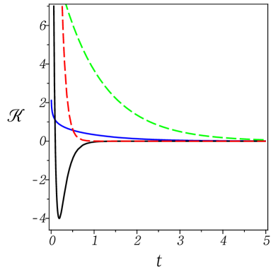
Figure 1: (Color online) Bath correlation function ${\mathcal{K}}={\mathcal{K}}_{\mu}^{(d)}(t)$ versus time $t$, given in (3a). Here we set $\hbar=k_{\mbox{\tiny B}}=M=\gamma_{\mbox{\tiny o}}=1$; solid line plotted at $T_{\mu}=1$ (low temperature) while dashed line at $T_{\mu}=10$ (high temperature). From top to bottom at $x=0.75$, 1st: (green dash: $\omega_{d}=1$); 2nd: (blue solid: $\omega_{d}=1$); 3rd: (red dash: $\omega_{d}=10$); 4th: (black solid: $\omega_{d}=10$). For the 1st, 2nd and 3rd lines, we have $\omega_{d}<\omega_{\mu}=2\pi\,T_{\mu}$. For the 4th, on the other hand, we have $\omega_{d}>\omega_{\mu}$, which gives rise to the low-temperature behavior of ${\mathcal{K}}_{\mu}^{(d)}(t)$ characterized by appearance of its negative-valued region; all four lines diverge at $t=0$ due to their behavior being proportional to $\delta(t)$ with $t\to 0$, directly obtained from (3).

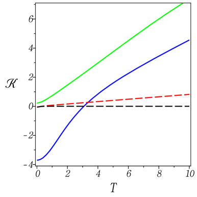
Figure 2: (Color online) Bath correlation function ${\mathcal{K}}={\mathcal{K}}_{\mu}^{(d)}(T)$ versus temperature $T$. Here we set $\hbar=k_{\mbox{\tiny B}}=M=\gamma_{\mbox{\tiny o}}=1$; solid line representing the typical early-time behavior, plotted at time $t=0.3$ while dashed line representing the late-time behavior, plotted at $t=2.5$. From top to bottom at $x=5$, 1st: (green solid: $\omega_{d}=1$); 2nd: (blue solid: $\omega_{d}=10$); 3rd: (red dash: $\omega_{d}=1$); 4th: (black dash: $\omega_{d}=10$). As demonstrated, the correlation function has no singularities at $\omega_{d}/\omega_{\mu}=1,2,\cdots$, where $\omega_{\mu}=2\pi x$.

where we introduce the effective frequency
$\omega_{\mu}=2\pi\,k_{\mbox{\tiny B}}T_{\mu}/\hbar$ as well as the Lerch function $\Phi(z,1,v)=v^{-1}\,{}_{2}F_{1}(1,v;1+v;z)$ [cf. (57)]. Here the singularities of $\cot(\pi y)$ at $y=1,2,\cdots$ disappear due to their cancellation with those of the two Lerch functions at the same points; behaviors of $K_{\mu}^{(d)}(t)$ versus time and temperature are plotted in Figs. 1 and 2, respectively. From this closed expression, we can straightforwardly recover, in the limit of $\omega_{\mu}\to\infty$, its classical counterpart given by $K_{\mbox{\tiny cl}}^{(d)}(t-t^{\prime})=k_{\mbox{\tiny B}}T_{\mu}M\,\gamma_{d}(t-t^{\prime})$, being well-known. In addition, by letting the cut-off frequency $\omega_{d}\to\infty$ corresponding to the Ohmic (or Markovian) damping $\gamma_{\mbox{\tiny o}}(t)=2\gamma_{\mbox{\tiny o}}\,\delta(t)$, the classical white-noise correlation function $K_{\mbox{\tiny cl}}^{({\mbox{\tiny o}})}(t-t^{\prime})$ immediately follows, too. In fact, Eq. (3a) will play critical roles in deriving analytical expressions of the steady-state heat current in Sects. 4-6.

3 Introduction of the steady-state heat current

We consider the average heat current flowing from a hot bath at temperature $T_{1}$ through the coupled harmonic chain to a cold bath at $T_{\scriptscriptstyle N}$ in the steady state $\hat{\rho}^{({\mbox{\tiny ss}})}(t)$, which is given by $\lim_{t\to\infty}\hat{\rho}(t)$ in the Schrödinger picture. Accordingly, the steady-state energy expectation value $\langle\hat{H}_{s}\rangle_{\hat{\rho}^{({\mbox{\tiny ss}})}}$ of the harmonic chain is required to remain unchanged with the time,

$$\frac{d}{dt}\left\langle\hat{H}_{s}\right\rangle_{\hat{\rho}^{({\mbox{\tiny ss}})}}\,=\,\mbox{Tr}\left\{\hat{H}_{s}\,\frac{d}{dt}\hat{\rho}^{({\mbox{\tiny ss}})}\right\}\,=\,0\,.$$ (4)

By substituting this into the Liouville equation $d\hat{\rho}^{({\mbox{\tiny ss}})}/dt=[\hat{H},\hat{\rho}^{({\mbox{\tiny ss}})}]/i\hbar$ and then applying the cyclic invariance of the trace, we can easily arrive at the expression

$$\mbox{Tr}\left\{\hat{J}_{{\mbox{\tiny in}}}^{({\scriptscriptstyle N})}\,\hat{\rho}^{({\mbox{\tiny ss}})}\right\}\,=\,-\mbox{Tr}\left\{\hat{J}_{{\mbox{\tiny out}}}^{({\scriptscriptstyle N})}\,\hat{\rho}^{({\mbox{\tiny ss}})}\right\}\,,$$ (5)

where we have two energy current operators denoted by $\hat{J}_{{\mbox{\tiny in}}}^{({\scriptscriptstyle N})}=[\hat{H}_{s},\hat{H}_{b_{1}-sb_{1}}]/i\hbar$ and $\hat{J}_{{\mbox{\tiny out}}}^{({\scriptscriptstyle N})}=[\hat{H}_{s},\hat{H}_{b_{\scriptscriptstyle N}-sb_{\scriptscriptstyle N}}]/i\hbar$. We identify the left-hand side of (5) as the steady-state input heat current ${\mathcal{J}}_{{\mbox{\tiny in}}}^{({\scriptscriptstyle N})}$ and the right-hand side as the output heat current $-{\mathcal{J}}_{{\mbox{\tiny out}}}^{({\scriptscriptstyle N})}$; due to the fact that $T_{1}\geq T_{{\scriptscriptstyle N}}$, we assume that ${\mathcal{J}}_{{\mbox{\tiny in}}}^{({\scriptscriptstyle N})}\geq 0$. Then both heat currents ${\mathcal{J}}_{{\mbox{\tiny in}}}^{({\scriptscriptstyle N})}$ and $-{\mathcal{J}}_{{\mbox{\tiny out}}}^{({\scriptscriptstyle N})}$, by construction, correspond to the input power from bath $1$ into the harmonic chain and the output power from the chain to bath $N$, respectively.

Now let us find an explicit expression of the steady-state heat current ${\mathcal{J}}_{{\mbox{\tiny in}}}^{({\scriptscriptstyle N})}$. We first substitute (1a)-(1b) and (a) into (5) and then rewrite the operator $\hat{P}_{1}\otimes\hat{x}_{1,\nu}$ as $\{\hat{P}_{1}\,,\,\hat{x}_{1,\nu}\}_{+}/2$, which will give rise to

$$\hat{J}_{{\mbox{\tiny in}}}^{({\scriptscriptstyle N})}\,=\,\frac{1}{2M}\left\{\hat{P}_{1}\,,\,-M\gamma(0)\,\hat{Q}_{1}+\sum_{\nu}c_{\nu}\,\hat{x}_{1,\nu}\right\}_{+}\,.$$ (6)

From the Langevin equation given in (2) with its damping term rewritten by integration by parts, we can also find that for a single Brownian oscillator (i.e., with chain length $N=1$) coupled directly to both separate baths,

$$\sum_{\nu}c_{\nu}\,\hat{x}_{\mu,\nu}(t) = \frac{M}{2}\,\ddot{\hat{Q}}_{1}(t)+\frac{M}{2}\,\left\{\Omega_{1}^{2}+2\,\gamma(0)\right\}\,\hat{Q}_{1}(t)+$$ (7)

$$\hat{\xi}_{b_{\mu}}(t)-\frac{1}{2}\,\left\{\hat{\xi}_{b_{1}}(t)+\hat{\xi}_{b_{1^{\prime}}}(t)\right\}\,,$$

where $\mu=1,1^{\prime}$ (i.e., $1^{\prime}\leftarrow N$), while for $N\geq 2$,

$$\sum c_{\nu}\,\hat{x}_{1,\nu}(t)\,=\,M\,\ddot{\hat{Q}}_{1}(t)\,+$$

$$\left\{M\Omega_{1}^{2}+\kappa_{1}+M\gamma(0)\right\}\,\hat{Q}_{1}(t)-\kappa_{1}\,\hat{Q}_{2}(t)\,.$$ (7a)

Next we substitute (7) into (6) and then into (5), as well as apply the cyclic invariance of the trace and $\hat{\rho}^{({\mbox{\tiny ss}})}=\lim_{t\to\infty}\hat{U}(t)\,\hat{\rho}(0)\,\hat{U}^{\dagger}(t)$ where $\hat{U}(t)=\exp(-i\hat{H}t/\hbar)$. This allows us to switch from the Schrödinger picture to the Heisenberg picture. Then the steady-state heat current turns out to be

$${\mathcal{J}}_{{\mbox{\tiny in}}}^{(1)} = \frac{1}{4M}\,\lim_{t\to\infty}\,\mbox{Tr}\left[\left\{\hat{P}_{1}(t)\,,\,M\,\ddot{\hat{Q}}_{1}(t)\,+\right.\right.$$ (8)

$$\left.\left.M\,\Omega_{1}^{2}\,\hat{Q}_{1}(t)\,+\,\hat{\xi}_{b_{1}}(t)\,-\,\hat{\xi}_{b_{1^{\prime}}}(t)\right\}_{+}\,\hat{\rho}(0)\right]$$

for $N=1$. In the same way, we can also find the corresponding expression of ${\mathcal{J}}_{{\mbox{\tiny out}}}^{(1)}$ independently, shown to be identical to (8) but with exchange of $\hat{\xi}_{b_{1}}(t)$ and $\hat{\xi}_{b_{1^{\prime}}}(t)$. Similarly, Eqs. (5), (6) and (7a) allow us to finally obtain the heat current

$${\mathcal{J}}_{{\mbox{\tiny in}}}^{({\scriptscriptstyle N})}\,= \,\frac{1}{2M}\,\lim_{t\to\infty}\,\mbox{Tr}\left[\left\{\hat{P}_{1}(t)\,,\,M\,\ddot{\hat{Q}}_{1}(t)\,+\right.\right.$$

$$\,\left.\left.(M\,\Omega_{1}^{2}+\kappa_{1})\,\hat{Q}_{1}(t)\,-\,\kappa_{1}\,\hat{Q}_{2}(t)\right\}_{+}\,\hat{\rho}(0)\right]$$ (8a)

for $N\geq 2$, as well as its counterpart ${\mathcal{J}}_{{\mbox{\tiny out}}}^{({\scriptscriptstyle N})}$, being identical to (8a) but with substitution of $\kappa_{1}\to\kappa_{{\scriptscriptstyle N}-1}$ and, for all remaining subscripts, $(1,2)\to(N,N-1)$. As shown, the key elements to the steady-state heat current are explicit expressions of $\{\hat{Q}_{1}(t),\hat{Q}_{2}(t),\hat{P}_{1}(t)\}$ in the limit of $t\to\infty$. We will below restrict our discussion of these expressions, for the sake of simplicity, mainly to the case of $\Omega_{1}=\cdots=\Omega_{\scriptscriptstyle N}=:\Omega$ and $\kappa_{1}=\cdots=\kappa_{{\scriptscriptstyle N}-1}=:\kappa$.

To derive an explicit form of each individual oscillator $\hat{Q}_{j}(t)$, we directly apply the Laplace transform to the Langevin equation (2). Let its Laplace transform $\underline{\hat{Q}_{j}}(s):={\mathcal{L}}\{\hat{Q}_{j}(t)\}(s)$, then giving rise to ${\mathcal{L}}\{\dot{\hat{Q}}_{j}(t)\}(s)=s\,\underline{\hat{Q}_{j}}(s)-\hat{Q}_{j}(0)$ and ${\mathcal{L}}\{\ddot{\hat{Q}}_{j}(t)\}(s)=s^{2}\,\underline{\hat{Q}_{j}}(s)-s\,\hat{Q}_{j}(0)-\dot{\hat{Q}}_{j}(0)$ ROB66 . Then we can easily obtain

$${\mathcal{B}}_{jk}(s)\,\underline{\hat{Q}_{k}}(s) = s\,\hat{Q}_{j}(0)+\dot{\hat{Q}}_{j}(0)+$$ (9)

$$\frac{1}{M}\,\left\{\underline{\hat{\xi}_{b_{1}}}(s)\,\delta_{j1}+\underline{\hat{\xi}_{b_{2}}}(s)\,\delta_{j{\scriptscriptstyle N}}\right\}\,,$$

where the Laplace-transformed fluctuating force

$$\underline{\hat{\xi}_{b_{\mu}}}(s)\,=\,\sum_{\nu=1}^{N_{b}}\frac{c_{\nu}}{s^{2}+\omega_{\nu}^{2}}\,\left\{s\,\hat{x}_{\mu,\nu}(0)+\frac{\hat{p}_{\mu,\nu}(0)}{m_{\nu}}\right\}\,,$$ (9a)

and the symmetric tridiagonal matrix ${\mathcal{B}}_{jk}(s)=s^{2}\,\delta_{jk}+s\,\bar{\gamma}(s)\,\Delta_{jk}+C_{jk}$ expressed in terms of
the Laplace-transformed damping kernel

$$\bar{\gamma}(s)\,=\,\frac{s}{M}\sum_{\nu=1}^{N_{b}}\frac{c_{\nu}^{2}}{m_{\nu}\,\omega_{\nu}^{2}}\,\frac{1}{s^{2}+\omega_{\nu}^{2}}\,.$$ (9b)

In the Drude-Ullersma model, the damping kernel $\bar{\gamma}(s)\to\bar{\gamma}_{d}(s)=\gamma_{\mbox{\tiny o}}\,\omega_{d}/(s+\omega_{d})$ WEI08 . Therefore, the central task to be undertaken is the determination of an explicit form of the inverse matrix $\hat{{\mathcal{B}}}^{-1}(s)=:\hat{{\mathcal{A}}}(s)$, which will be performed below for individual chain lengths $N$.

4 Steady-state heat current for the case of $N=1$

We begin with the simplest case of $N=1$, in which a single oscillator is coupled directly to two separate baths at different temperatures. As well-known, the matrix $\hat{{\mathcal{A}}}(s)$ then reduces to $M\bar{\chi}(s)$, where

$$\bar{\chi}(s)\,=\,\frac{1}{M}\,\frac{1}{s^{2}\,+\,\Omega^{2}\,+\,2\,s\,\bar{\gamma}(s)}\,,$$ (10)

corresponding to the dynamic susceptibility in the frequency domain, given by $\tilde{\chi}(\omega)\leftarrow\bar{\chi}(s)$ with $s\to-i\omega+0^{+}$ WEI08 . In the Drude-Ullersma model, Eq. (10) reduces to

$$\bar{\chi}_{d}(s)\,=\,\frac{(s+\omega_{d})/M}{h_{1}(s)}\,,$$ (10a)

where $h_{1}(s)=s^{3}+\omega_{d}\,s^{2}+(\Omega^{2}+\gamma_{\mbox{\tiny o}}^{\prime}\,\omega_{d})\,s+\Omega^{2}\,\omega_{d}$, with $\gamma_{\mbox{\tiny o}}^{\prime}=2\gamma_{\mbox{\tiny o}}$ and all its coefficients being positive-valued. Accordingly, this cubic polynomial can be factorized as $(s+z_{0})(s+z_{1})(s+z_{2})$, where $\mbox{Re}(z_{0}),\mbox{Re}(z_{1}),\mbox{Re}(z_{2})>0$, through the symmetric relations

$$z_{0}+z_{1}+z_{2} = \omega_{d}\;,\;\Omega^{2}+\gamma_{\mbox{\tiny o}}^{\prime}\,\omega_{d}\,=\,z_{0}\,(z_{1}+z_{2})+z_{1}\,z_{2}\;,$$

$$\Omega^{2}\,\omega_{d} = z_{0}\,z_{1}\,z_{2}\,;$$ (11)

$(z_{0},z_{1},z_{2})$ can equivalently be rewritten as $({\mathbf{w}}_{0},z_{0},\gamma)$, where FOR06

$$\Omega^{2}\,= \,\left({\mathbf{w}}_{0}\right)^{2}\;\frac{z_{0}}{z_{0}\,+\,\gamma}\;\;\;,\;\;\;\omega_{d}\,=\,z_{0}\,+\,\gamma\;\;\;,$$

$$\,\gamma_{\mbox{\tiny o}}^{\prime}\,=\,\gamma\,\frac{z_{0}\,(z_{0}\,+\,\gamma)\,+\,\left({\mathbf{w}}_{0}\right)^{2}}{(z_{0}\,+\,\gamma)^{2}}\,;$$ (4a)

then these lead to $z_{1}=\gamma/2+i{\mathbf{w}}_{1}$ and $z_{2}=\gamma/2-i{\mathbf{w}}_{1}$ with ${\mathbf{w}}_{1}=\sqrt{({\mathbf{w}}_{0})^{2}-(\gamma/2)^{2}}$. The parameters $(z_{0},z_{1},z_{2})$ will be useful for a compact expression of the steady-state heat current ${\mathcal{J}}_{{\mbox{\tiny in}}}^{(1)}$ [cf. (4)]. In fact, these can be explicitly expressed in terms of $(\Omega,\omega_{d},\gamma_{\mbox{\tiny o}})$ by the cubic formula, as well-known JAP00 .

Now let us find an explicit expression of the single oscillator $\hat{Q}_{1}(t)$ in the limit of $t\to\infty$ by considering the equation of its Laplace transform $\underline{\hat{Q}_{1}}(s)$ given in (9). This can be efficiently carried out with the aid of the final value theorem of the Laplace transform COH07 ; it reads as $\lim_{t\to\infty}f(t)=\lim_{s\to 0}sF(s)$, where $F(s)={\mathcal{L}}\{f(t)\}(s)$, upon condition that all poles of $F(s)$, except $s=0$, have negative real parts, i.e., if $sF(s)$ is analytic on the imaginary axis and in the right half-plane. By noting from (10a) the fact that this condition is met by $\bar{\chi}_{d}(s)$ and so $\lim_{s\to 0}s\,\bar{\chi}_{d}(s)=\lim_{s\to 0}s^{2}\,\bar{\chi}_{d}(s)=0$, we can easily obtain from (9) the expression

$$\lim_{t\to\infty}\hat{Q}_{1}(t)\,=\,\lim_{t\to\infty}\int_{0}^{t}dt^{\prime}\,\chi_{d}(t-t^{\prime})\,\left\{\hat{\xi}_{b_{1}}(t^{\prime})+\hat{\xi}_{b_{1^{\prime}}}(t^{\prime})\right\}\,,$$ (12)

where the response function ILK10

$$\chi_{d}(t)\,=\,{\mathcal{L}}^{-1}\{\bar{\chi}_{d}(s)\}\,=\,-\frac{1}{M}\,\times$$ (12a)

$$\frac{\left(z_{1}^{2}-z_{2}^{2}\right)\,e^{-z_{0}\,t}\,+\,\left(z_{2}^{2}-z_{0}^{2}\right)\,e^{-z_{1}\,t}\,+\,\left(z_{0}^{2}-z_{1}^{2}\right)\,e^{-z_{2}\,t}}{\left(z_{0}-z_{1}\right)\,\left(z_{1}-z_{2}\right)\,\left(z_{2}-z_{0}\right)}\,.$$

For the sake of comparison with (12), it is also worthwhile to mention that both fluctuating forces $\underline{\hat{\xi}_{b_{1}}}(s)$ and $\underline{\hat{\xi}_{b_{1^{\prime}}}}(s)$, as shown in (9a), do not meet the prerequisite for applying the final value theorem, though, and so it turns out that

$$\lim_{t\to\infty}\,\hat{Q}_{1}(t)\,\neq\,\lim_{s\to 0}\,s\,\bar{\chi}_{d}(s)\,\left\{\underline{\hat{\xi}_{b_{1}}}(s)+\underline{\hat{\xi}_{b_{1^{\prime}}}}(s)\right\}\,.$$ (12b)

Similarly, it appears from $\hat{P}_{1}(t)=M\dot{\hat{Q}}_{1}(t)$ and $\chi_{d}(0)=0$ that

$$\lim_{t\to\infty}\hat{P}_{1}(t)\,=\,M\,\lim_{t\to\infty}\int_{0}^{t}dt^{\prime}\,\left\{\frac{\partial}{\partial t}\chi_{d}(t-t^{\prime})\right\}\,\left\{\hat{\xi}_{b_{1}}(t^{\prime})+\hat{\xi}_{b_{1^{\prime}}}(t^{\prime})\right\}\,.$$ (13)

Now we are ready to derive an explicit expression of the steady-state current. Substituting (12) and (13) into (8), we first obtain the steady-state expectation value

$$\left\langle\left\{\hat{P}_{1}(t)\,,\,\hat{Q}_{1}(t)\right\}_{+}\right\rangle^{({\mbox{\tiny ss}})}\,=\,2M\,\lim_{t\to\infty}\int_{0}^{t}d\tau\int_{0}^{t}d\tau^{\prime}\chi_{d}(t-\tau)$$

$$\times\left\{\frac{\partial}{\partial t}\chi_{d}(t-\tau^{\prime})\right\}\,\left\{K_{1}^{(d)}(\tau-\tau^{\prime})\,+\,K_{1^{\prime}}^{(d)}(\tau-\tau^{\prime})\right\}\,.$$ (14)

Plugging subsequently into this expression both (12a) and (3a) with (57), and then using GRA07

$$\lim_{t\to\infty}\int_{0}^{t}d\tau\,e^{-\alpha^{\prime\prime}\,(t-\tau)}\int_{0}^{t}d\tau^{\prime}\,e^{-\alpha^{\prime}\,(t-\tau^{\prime})}\,e^{-\alpha\,|\tau-\tau^{\prime}|}$$ (15)

$$= \frac{\alpha^{\prime\prime}+\alpha^{\prime}+2\alpha}{(\alpha^{\prime\prime}+\alpha^{\prime})\,(\alpha^{\prime}+\alpha)\,(\alpha+\alpha^{\prime\prime})}\,,$$

where $\alpha=\omega_{d}$ or $n\omega_{\mu}$ with $n=0,1,2,\cdots$, we can explicitly evaluate the double integral in (4), which turns out to vanish due to the symmetric structure of $\chi_{d}(t)$ in $(z_{0},z_{1},z_{2})$. Next, taking into account the fact that $\ddot{\hat{Q}}_{1}(t)=\dot{\hat{P}}_{1}(t)/M$ and $d{\chi}_{d}(0)/dt=1/M$, we can also find that $\langle\{\hat{P}_{1}(t)\,,\,\ddot{\hat{Q}}_{1}(t)\}_{+}\rangle^{({\mbox{\tiny ss}})}=0$. Then the formal expression of the heat current given in (8) is simplified as

$${\mathcal{J}}_{{\mbox{\tiny in}}}^{(1)}\,=\,\frac{1}{4M}\,\left\langle\left\{\hat{P}_{1}(t)\,,\,\hat{\xi}_{b_{1}}(t)-\hat{\xi}_{b_{1^{\prime}}}(t)\right\}_{+}\right\rangle^{({\mbox{\tiny ss}})}\,.$$ (16)

Along the same line, we can also obtain the expression for ${\mathcal{J}}_{{\mbox{\tiny out}}}^{(1)}$, identical to (16) but with exchange of $\hat{\xi}_{b_{1}}(t)$ and $\hat{\xi}_{b_{1^{\prime}}}(t)$, which immediately verifies that ${\mathcal{J}}_{{\mbox{\tiny out}}}^{(1)}=-{\mathcal{J}}_{{\mbox{\tiny in}}}^{(1)}$ indeed. In the equilibrium state given by $\beta_{1}=\beta_{1^{\prime}}$, the heat current vanishes, as expected. We can also expect, from (13) and (16), the appearance of quantum behaviors of the heat current ${\mathcal{J}}_{{\mbox{\tiny in}}}^{(1)}$ due to the quantum nature of the bath correlation function $K_{\mu}^{(d)}(t-t^{\prime})$ given in (3)-(3a).

After some algebraic manipulations, every single step of which is provided in detail in Appendix B, Eq. (16) finally reduces to the exact expression

$${\mathcal{J}}_{{\mbox{\tiny in}}}^{(1)}\;=\;\frac{\hbar\,\gamma\,\{z_{0}\,\omega_{d}+({\mathbf{w}}_{0})^{2}\}}{8\pi}\,\times$$ (17)

$$\sum_{\underline{j}=0}^{2}\frac{z_{\underline{j}}\cdot(\omega_{d}-z_{\underline{j}})}{(z_{\underline{j}}-z_{\underline{j+1}})\cdot(z_{\underline{j}}-z_{\underline{j+2}})}\,\left\{\Upsilon_{{\scriptscriptstyle\beta_{1}}}(z_{\underline{j}})-\Upsilon_{{\scriptscriptstyle\beta_{1^{\prime}}}}(z_{\underline{j}})\right\}$$

in terms of the parameters $({\mathbf{w}}_{0},z_{0},\gamma)$ given in (a), where $\underline{j}=j\,(\mbox{mod}\;3)$. Here,

$$\Upsilon_{{\scriptscriptstyle\beta}}(z_{\underline{j}}) := \frac{-\pi\,\cot\left(\frac{\beta\hbar\omega_{d}}{2}\right)+\psi\left(-\frac{\beta\hbar\omega_{d}}{2\pi}\right)-\psi\left(\frac{\beta\hbar z_{\underline{j}}}{2\pi}\right)}{\omega_{d}\,+\,z_{\underline{j}}}$$ (18)

$$-\,\frac{\psi\left(\frac{\beta\hbar\omega_{d}}{2\pi}\right)-\psi\left(\frac{\beta\hbar z_{\underline{j}}}{2\pi}\right)}{\omega_{d}\,-\,z_{\underline{j}}}\,,$$

where the digamma function $\psi(y)=d\,\ln\Gamma(y)/dy$ ABS74 . With the help of (4)-(a) and (67)-(68) as well as the relation given by $-\pi\cot(y)+\psi(-y/\pi)=\psi(y/\pi)+\pi/y$, Eq. (17) can be rewritten as a compact expression

$${\mathcal{J}}_{{\mbox{\tiny in}}}^{(1)}\,=\,\frac{\hbar\omega_{d}^{2}\,\gamma_{\mbox{\tiny o}}}{2\pi}\left[\frac{\omega_{d}^{2}\cdot(g_{{\scriptscriptstyle\beta_{1}}}-g_{{\scriptscriptstyle\beta_{1^{\prime}}}})}{h_{1}(\omega_{d})}\,+\right.$$

$$\left.\sum_{\underline{j}=0}^{2}\frac{z_{\underline{j}}^{2}\cdot\{\psi_{{\scriptscriptstyle\beta_{1}}}(z_{\underline{j}})-\psi_{{\scriptscriptstyle\beta_{1^{\prime}}}}(z_{\underline{j}})\}}{(z_{\underline{j}}-z_{\underline{j+1}})(z_{\underline{j}}-z_{\underline{j+2}})(z_{\underline{j}}+\omega_{d})}\right]\,,$$ (19)

where $\psi_{{\scriptscriptstyle\beta}}(y):=\psi(\beta\hbar y/2\pi)$, and
$g_{{\scriptscriptstyle\beta}}:=-\{\psi_{{\scriptscriptstyle\beta}}(\omega_{d})+2\pi/\beta\hbar\omega_{d}\}$.

Now we consider the semiclassical behavior of this heat current by expanding the digamma functions such that in the limit of $\beta\hbar\to 0$,

$${\mathcal{J}}_{{\mbox{\tiny in}}}^{(1)}\,=\,{\mathcal{J}}_{{\mbox{\tiny cl}}}^{(1)}\cdot\left[1\,-\,\frac{\hbar^{2}\,\beta_{1}\,\beta_{1^{\prime}}}{12}\,(\Omega^{2}+\gamma_{\mbox{\tiny o}}\,\omega_{d})\,+\right.$$

$$\frac{\hbar^{4}\,\beta_{1}\,\beta_{1^{\prime}}\,(\beta_{1}^{2}+\beta_{1}\,\beta_{1^{\prime}}+\beta_{1^{\prime}}^{2})}{2^{4}\cdot 3^{2}\cdot 5}\,\times$$ (20)

$$\left.\left\{\Omega^{4}+\gamma_{\mbox{\tiny o}}\,\omega_{d}\,(3\,\Omega^{2}+2\,\gamma_{\mbox{\tiny o}}\,\omega_{d}+\omega_{d}^{2})\right\}\,+\,{\mathcal{O}}\left\{(\beta\hbar)^{6}\right\}\right]\,,$$

expressed in terms of the original input parameters
$(\Omega,\omega_{d},\gamma_{\mbox{\tiny o}})$ only, the derivation of which is provided in Appendix B). Here the leading term

$${\mathcal{J}}_{{\mbox{\tiny cl}}}^{(1)}\,=\,\frac{\gamma_{\mbox{\tiny o}}\,\omega_{d}^{2}}{2\,(\Omega^{2}+\gamma_{\mbox{\tiny o}}\,\omega_{d}+\omega_{d}^{2})}\,\left(\frac{1}{\beta_{1}}-\frac{1}{\beta_{1^{\prime}}}\right)$$ (4a)

corresponds to the classical counterpart to ${\mathcal{J}}_{{\mbox{\tiny in}}}^{(1)}$, being valid in the high-temperature limit. In the Ohmic limit $\omega_{d}\to\infty$, this classical value reduces to the well-known expression given by ${\mathcal{J}}_{{\mbox{\tiny cl}}}^{({\mbox{\tiny o}})}=(\gamma_{\mbox{\tiny o}}/2)\cdot(1/\beta_{1}-1/\beta_{1^{\prime}})$. On the other hand, the steady-state heat current in (4) reveals its different behavior in the low-temperature limit of $\beta\hbar\to\infty$, explicitly given by (cf. Appendix B)

$${\mathcal{J}}_{{\mbox{\tiny in}}}^{(1)} = \frac{\hbar\omega_{d}^{4}\,\gamma_{\mbox{\tiny o}}}{4\pi}\sum_{n=0}^{\infty}\frac{B_{2n+4}}{n+2}\cdot\left(\frac{2\pi}{\hbar\omega_{d}}\right)^{2n+4}\,\times$$

$$\left(\frac{1}{\beta_{1}^{2n+4}}\,-\,\frac{1}{\beta_{1^{\prime}}^{2n+4}}\right)\sum_{p=0}^{2n+1}\left.\frac{\omega_{d}^{p}}{p!}\cdot\left\{\frac{1}{h_{1}(s)}\right\}^{(p)}\right|_{s=0}$$

expressed in terms of the Bernoulli numbers $B_{2n}$, where $\{\cdots\}^{(p)}$ denotes the $p$-th derivative. We see that in this genuine quantum regime, the heat current is not directly proportional to the bath-temperature difference any longer. With $B_{4}=-1/30$, the leading term $n=0$ of (4) easily reduces to the input power

$${\mathcal{J}}_{{\mbox{\tiny qm}}}^{(1,0)}\,=\,\frac{2\,\pi^{3}\,\gamma_{\mbox{\tiny o}}^{2}\,k_{\mbox{\tiny B}}^{4}}{15\,\hbar^{3}\,\Omega^{4}}\,\left(T_{1}^{4}\,-\,T_{1^{\prime}}^{4}\right)\,,$$ (4a)

being $\omega_{d}$-independent. This is the same in form of the temperature dependency as the well-known Stefan-Boltzmann law for the power radiated from a black-body LAN89 .

As a result, it turns out that Fourier’s law of heat conduction is not valid even for the case of $N=1$, especially in the low-temperature limit. The behaviors of ${\mathcal{J}}_{{\mbox{\tiny in}}}^{(1)}$ versus the “hot-bath” temperature $T_{1}$ are plotted in Figs. 3 and 4, where two different “cold-bath” temperatures $T_{1^{\prime}}$ are imposed in the low-temperature and the high-temperature regime, respectively; in the weak-coupling limit imposed by $\gamma_{\mbox{\tiny o}}\ll\Omega$, the low-magnitude heat current is observed indeed. In the next section, the heat current ${\mathcal{J}}_{{\mbox{\tiny in}}}^{(2)}$ for $N=2$ will explicitly come out by applying its formal expression in (8a), valid for $N\geq 2$, rather than the one in (8) used for $N=1$.

5 Steady-state heat current for the case of $N=2$

We now consider the case of $N=2$. To efficiently proceed with the determination of an explicit form of the inverse matrix $\hat{{\mathcal{B}}}^{-1}(s)$, we first diagonalize the tridiagonal matrix $\hat{{\mathcal{B}}}(s)$. To do so, we introduce the normal coordinates $\{\underline{\hat{{\mathcal{Q}}}_{j}}(s)\}$ of the isolated chain $\hat{H}_{s}$ given in (1a), which satisfy $\underline{\hat{Q}_{j}}(s)=O_{jk}\underline{\hat{{\mathcal{Q}}}_{k}}(s)$ and $(\hat{O}^{t}\,\hat{C}\,\hat{O})_{jk}=\bar{\Omega}_{k}^{2}\,\delta_{jk}$ with $\hat{O}^{t}\,\hat{O}=\hat{O}\,\hat{O}^{t}=\openone_{\scriptscriptstyle N}$ GAU07 . Eq. (9) is then rewritten as

$${\mathfrak{B}}_{jk}(s)\,\underline{\hat{{\mathcal{Q}}}_{k}}(s) = s\hat{{\mathcal{Q}}}_{j}(0)\,+\,\dot{\hat{{\mathcal{Q}}}}_{j}(0)\,+$$ (22)

$$\frac{1}{M}\left\{\underline{\hat{\xi}_{b_{1}}}(s)\,O_{1j}+\underline{\hat{\xi}_{b_{2}}}(s)\,O_{{\scriptscriptstyle N}j}\right\}\,,$$

where the matrix

$${\mathfrak{B}}_{jk}(s)\,:= \,\left(\hat{O}^{t}\,\hat{\mathcal{B}}\,\hat{O}\right)_{jk}(s)\,=\,\left(s^{2}\,+\,\bar{\Omega}_{k}^{2}\right)\,\delta_{jk}\,+$$

$$\,s\,\bar{\gamma}(s)\,\left(\delta_{jk}\,-\,\sum_{n=2}^{N-1}O_{nj}\,O_{nk}\right)\,,$$ (22a)

being, in fact, of diagonal form for $N=2$. For the case of $\Omega_{1}=\Omega_{2}=:\Omega$ to be considered here, it easily turns out that $\bar{\Omega}_{1}=\Omega$ and $\bar{\Omega}_{2}=(\Omega^{2}+2\kappa/M)^{1/2}$ as well as

$$\hat{O}\,=\,\frac{1}{\sqrt{2}}\left(\begin{array}[]{rr}1&1\\ 1&-1\end{array}\right)\,,$$ (25)

which is a simple constant matrix; for an isolated chain with $N\geq 3$, in comparison, it is straightforward to verify that the matrix elements $O_{jk}$ are not mere constants but functions of $s$ KIM13 . Then the inverse matrix $\hat{\mathfrak{B}}^{-1}(s)$ appears as a diagonal form with $({\mathfrak{B}}^{-1})_{11}(s)=M\bar{\chi}_{1}(s)$ and $({\mathfrak{B}}^{-1})_{22}(s)=M\bar{\chi}_{2}(s)$, where each of $\bar{\chi}_{\mu}(s)$ with $\mu=1,2$ corresponds to $\bar{\chi}(s)$ given in (10) used for $N=1$, with substitution of $\Omega\to\bar{\Omega}_{\mu}$.

We are now ready to apply to each of these two diagonal elements the same technique as for $N=1$. Then it turns out, with the help of (25), that

$$\lim_{t\to\infty}\hat{Q}_{1}(t) = \frac{1}{2}\,\lim_{t\to\infty}\int_{0}^{t}d\tau\sum_{\mu=1}^{2}\,\chi_{\mu}(t-\tau)\,\times$$ (26a)

$$\left\{\hat{\xi}_{b_{1}}(\tau)-(-1)^{\mu}\,\hat{\xi}_{b_{2}}(\tau)\right\}$$

$$\lim_{t\to\infty}\hat{Q}_{2}(t) = \frac{1}{2}\,\lim_{t\to\infty}\int_{0}^{t}d\tau\sum_{\mu=1}^{2}\,\chi_{\mu}(t-\tau)\,\times$$ (26b)

$$\left\{\hat{\xi}_{b_{2}}(\tau)-(-1)^{\mu}\,\hat{\xi}_{b_{1}}(\tau)\right\}\,.$$

To explicitly evaluate the formal expression of the heat current ${\mathcal{J}}_{{\mbox{\tiny in}}}^{(2)}$ in (8a), we first focus on the steady-state expectation value

$$\left\langle\left\{\hat{P}_{1}(t)\,,\,\hat{Q}_{1}(t)\right\}_{+}\right\rangle^{({\mbox{\tiny ss}})}\,=\,\frac{M}{2}\,\lim_{t\to\infty}\int_{0}^{t}d\tau\int_{0}^{t}d\tau^{\prime}$$ (27)

$$\frac{\partial}{\partial t}\left\{\chi_{1}(t-\tau)\,\chi_{2}(t-\tau^{\prime})\right\}\,\left\{K_{1}^{(d)}(\tau-\tau^{\prime})\,-\,K_{2}^{(d)}(\tau-\tau^{\prime})\right\}\,.$$

By means of the same technique as for the case of $N=1$, we can straightforwardly show that this vanishes indeed. Likewise, it also turns out that $\langle\{\hat{P}_{1}(t)\,,\,\ddot{\hat{Q}}_{1}(t)\}_{+}\rangle^{({\mbox{\tiny ss}})}=0$. Similarly, the last needed expectation value

$$\left\langle\left\{\hat{P}_{1}(t)\,,\,\hat{Q}_{2}(t)\right\}_{+}\right\rangle^{({\mbox{\tiny ss}})}\,=\,\frac{M}{2}\,\lim_{t\to\infty}\int_{0}^{t}d\tau\int_{0}^{t}d\tau^{\prime}$$

$$\left[\chi_{1}(t-\tau)\,\{\partial_{t}\,\chi_{2}(t-\tau^{\prime})\}\,-\,\{\partial_{t}\,\chi_{1}(t-\tau)\}\,\chi_{2}(t-\tau^{\prime})\right]\,\times$$

$$\left[K_{1}^{(d)}(\tau-\tau^{\prime})\,-\,K_{2}^{(d)}(\tau-\tau^{\prime})\right]\,\neq\,0$$ (28)

can be evaluated in closed form (cf. Appendix C). Substituting this form into (8a), we can immediately arrive at an exact expression of the steady-state heat current

$${\mathcal{J}}_{{\mbox{\tiny in}}}^{(2)}\,=\,-\frac{\kappa}{2M}\,\left\langle\left\{\hat{P}_{1}(t)\,,\,\hat{Q}_{2}(t)\right\}_{+}\right\rangle^{({\mbox{\tiny ss}})}\,=\,\frac{\hbar\,\omega_{d}^{2}\,\kappa\,\gamma_{\mbox{\tiny o}}}{4\pi M}\,\times$$

$$\sum_{\underline{j}=0}^{2}\left(\left[\frac{(\omega_{d}^{2}-z_{\underline{j}}^{2})\cdot z_{\underline{j}}\cdot\{\Upsilon_{{\scriptscriptstyle\beta_{1}}}(z_{\underline{j}})-\Upsilon_{{\scriptscriptstyle\beta_{2}}}(z_{\underline{j}})\}}{(z_{\underline{j}}-z_{\underline{j+1}})\cdot(z_{\underline{j}}-z_{\underline{j+2}})\cdot h_{12}(z_{\underline{j}})}\right]\,-\right.$$

$$\left.\left[z_{\underline{j}}\to z_{\underline{j}}^{\prime}\,;\,h_{12}(z_{\underline{j}})\to h_{11}(z_{\underline{j}}^{\prime})\right]\right)\,,$$ (29)

where the parameters $z_{\underline{j}}$’s are identical to $(z_{0},z_{1},z_{2})$ given in (4) but with substitution of $\Omega\to\bar{\Omega}_{1}$, and so are $z_{\underline{j}}^{\prime}$’s with $\Omega\to\bar{\Omega}_{2}$. The function $h_{11}(z_{\underline{j}}^{\prime}):=h_{1}(z_{\underline{j}}^{\prime})$ with $\Omega\to\bar{\Omega}_{1}$, and $h_{12}(z_{\underline{j}}):=h_{1}(z_{\underline{j}})$ with $\Omega\to\bar{\Omega}_{2}$; by construction, $h_{11}(-z_{\underline{j}})=h_{12}(-z_{\underline{j}}^{\prime})=0$. As given in (4) for $N=1$, Eq. (5) can finally be rewritten as

$${\mathcal{J}}_{{\mbox{\tiny in}}}^{(2)} = -\frac{\kappa^{2}\gamma_{\mbox{\tiny o}}}{M^{2}}\,\left(\mbox{\={I}}_{2}\right)\cdot\left(\frac{1}{\beta_{1}}-\frac{1}{\beta_{2}}\right)\,+\,\frac{\hbar\,\omega_{d}^{2}\,\kappa\,\gamma_{\mbox{\tiny o}}}{2\pi M}\,\times$$ (30)

$$\sum_{\underline{j}=0}^{2}\left[\left\{\frac{z_{\underline{j}}^{2}\cdot\{\psi_{{\scriptscriptstyle\beta_{1}}}(z_{\underline{j}})-\psi_{{\scriptscriptstyle\beta_{2}}}(z_{\underline{j}})\}}{(z_{\underline{j}}-z_{\underline{j+1}})\cdot(z_{\underline{j}}-z_{\underline{j+2}})\cdot h_{12}(z_{\underline{j}})}\right\}\,-\right.$$

$$\left.\left\{z_{\underline{j}}\to z_{\underline{j}}^{\prime}\,;\,h_{12}(z_{\underline{j}})\to h_{11}(z_{\underline{j}}^{\prime})\right\}\right]\,.$$

Here $\left(\mbox{\={I}}_{2}\right):=\omega_{d}^{2}\cdot f_{\kappa}/(2\,\lambda_{\kappa})$, where $f_{\kappa}=\Omega^{2}+\kappa/M+\omega_{d}^{2}$ and

$$\lambda_{\kappa}\;=\;2\,(\Omega^{2}+\omega_{d}^{2}+\gamma_{\mbox{\tiny o}}\,\omega_{d})\left(\frac{\kappa}{M}\right)^{3}\,+\,\left(\Omega^{4}+2\,\Omega^{2}\gamma_{\mbox{\tiny o}}\,\omega_{d}\,+\right.$$

$$\left.2\,\Omega^{2}\,\omega_{d}^{2}-2\,\gamma_{\mbox{\tiny o}}\,\omega_{d}^{3}+\omega_{d}^{4}\right)\left(\frac{\kappa}{M}\right)^{2}\,+\,4\,\gamma_{\mbox{\tiny o}}^{2}\,\omega_{d}^{4}\left(\frac{\kappa}{M}\right)\,+\,4\,\Omega^{2}\,\gamma_{\mbox{\tiny o}}^{2}\,\omega_{d}^{4}\,.$$ (30a)

Now we apply to the exact expression given in (30) the same technique as provided for (4), in order to study its semiclassical behavior. Then it turns out that

$${\mathcal{J}}_{{\mbox{\tiny in}}}^{(2)}\,=\,{\mathcal{J}}_{{\mbox{\tiny cl}}}^{(2)}\cdot\left[1\,-\,\frac{\hbar^{2}\,\beta_{1}\,\beta_{2}}{12}\,\frac{v_{\kappa}}{f_{\kappa}}\,-\right.$$ (31)

$$\left.\frac{\hbar^{4}\,\beta_{1}\,\beta_{2}\,(\beta_{1}^{2}+\beta_{1}\,\beta_{2}+\beta_{2}^{2})}{2^{3}\cdot 3^{2}\cdot 5}\,\frac{\Omega^{4}\,\omega_{d}}{f_{\kappa}}\,+\,{\mathcal{O}}\left\{(\beta\hbar)^{6}\right\}\right]\,,$$

where $v_{\kappa}:=(2\,\Omega^{2}+2\,\gamma_{\mbox{\tiny o}}\,\omega_{d}+\omega_{d}^{2})\cdot\kappa/M+\Omega^{4}+\Omega^{2}\,\omega_{d}\,(2\,\gamma_{\mbox{\tiny o}}+\omega_{d})$. Here, the leading term is given by the classical counterpart

$${\mathcal{J}}_{{\mbox{\tiny cl}}}^{(2)}\,=\,\frac{\kappa^{2}\gamma_{\mbox{\tiny o}}}{M^{2}}\,\left(\mbox{\={I}}_{2}\right)\cdot\left(\frac{1}{\beta_{1}}-\frac{1}{\beta_{2}}\right)\,.$$ (31a)

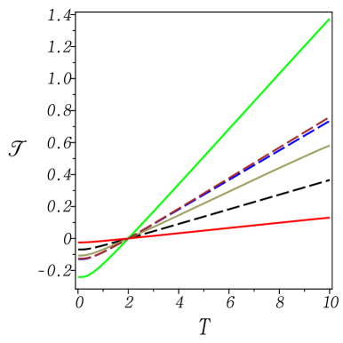
Figure 6: (Color online) The same plot as in Fig. 5, in the high-temperature regime where the cold-bath temperature is imposed by $T_{2}=2$. As such, ${\mathcal{J}}={\mathcal{J}}_{{\mbox{\tiny in}}}^{(2)}(T,2)=0$ at the thermal equilibrium point, $T=2$. In the region of $T\geq 2$ the heat current reveals the behavior of its classical counterpart, being proportional to $T-T_{2}$, while for $T<2$ it is negative-valued. As shown, we have the same lines for $T\geq T_{2}$ as in Fig. 5, except that the 1st top dashed line (at $x=10$): (brown: $\gamma_{\mbox{\tiny o}}=0.2$, and $\kappa=2.2$ instead of $1.5$), and 2nd top dash: (blue: $\gamma_{\mbox{\tiny o}}=0.2$ and $\kappa=1$), i.e., for $\gamma_{\mbox{\tiny o}}=0.2$ the maximum heat current appears at $\kappa=1=\kappa_{\mbox{\tiny R}}$ while with further increase of $\kappa>\kappa_{\mbox{\tiny R}}$, the current decreases very slowly.

The behaviors of ${\mathcal{J}}_{{\mbox{\tiny in}}}^{(2)}$ in the low-temperature and the high-temperature regime are plotted in Figs. 5 and 6, respectively; as demonstrated, they are consistent with the behaviors of ${\mathcal{J}}_{{\mbox{\tiny in}}}^{(1)}$. Here the weak-coupling limit is imposed by $\kappa/M,\gamma_{\mbox{\tiny o}}^{2}\ll\Omega^{2}$. Along the same line as (27)-(5), we can also obtain that

$$\left\langle\left\{\hat{P}_{2}(t)\,,\,\hat{Q}_{2}(t)\right\}_{+}\right\rangle^{({\mbox{\tiny ss}})} = -\left\langle\left\{\hat{P}_{1}(t)\,,\,\hat{Q}_{1}(t)\right\}_{+}\right\rangle^{({\mbox{\tiny ss}})}$$ (32a)

$$\left\langle\left\{\hat{P}_{2}(t)\,,\,\ddot{\hat{Q}}_{2}(t)\right\}_{+}\right\rangle^{({\mbox{\tiny ss}})} = -\left\langle\left\{\hat{P}_{1}(t)\,,\,\ddot{\hat{Q}}_{1}(t)\right\}_{+}\right\rangle^{({\mbox{\tiny ss}})}$$ (32b)

$$\left\langle\left\{\hat{P}_{2}(t)\,,\,\hat{Q}_{1}(t)\right\}_{+}\right\rangle^{({\mbox{\tiny ss}})} = -\left\langle\left\{\hat{P}_{1}(t)\,,\,\hat{Q}_{2}(t)\right\}_{+}\right\rangle^{({\mbox{\tiny ss}})}\,.$$ (32c)

From this, it follows that ${\mathcal{J}}_{{\mbox{\tiny out}}}^{(2)}=-{\mathcal{J}}_{{\mbox{\tiny in}}}^{(2)}$ indeed. We see from (31)-(31a) that ${\mathcal{J}}_{{\mbox{\tiny in}}}^{(2)}\to 0$ for $\kappa\to 0$, and so there can be no sufficiently high output power in the weak-coupling regime, as expected. Finally we remark for a later purpose that the steady-state heat current ${\mathcal{J}}_{{\mbox{\tiny in}}}^{(2)}$ was rigorously treated based on the two uncoupled normal modes, each of which was thoroughly studied for ${\mathcal{J}}_{{\mbox{\tiny in}}}^{(1)}$ already in Sect. 4.

6 Steady-state heat current for the case of $N\geq 3$

We first need to point out that the matrix $\hat{{\mathfrak{B}}}(s)$ given in (22a) is not of diagonal form for $N\geq 3$ and neither is its inverse. Therefore, the normal-coordinate technique provided for $N=2$ cannot straightforwardly be applied any longer. Instead, we adopt a different approach to the determination of an explicit form of $\hat{{\mathcal{B}}}^{-1}(s)=\hat{{\mathcal{A}}}(s)$, developed in USM94 ; YUE06 ; given an $N\times N$ symmetric tridiagonal matrix

$$\hat{{\mathcal{B}}}(s)\;=\;\left(\begin{array}[]{ccccccc}a&c&0&0&\cdots&0&0\\ c&b&c&0&\cdots&0&0\\ 0&c&b&c&\cdots&0&0\\ 0&0&c&b&\cdots&0&0\\ \cdots&&\cdots&&\cdots&&\cdots\\ 0&0&0&\cdots&c&b&c\\ 0&0&0&\cdots&0&c&a\end{array}\right)\,,$$ (33)

where

$$a\,:=\,s^{2}+s\,\bar{\gamma}(s)+\Omega^{2}+\frac{\kappa}{M}$$

$$b\,:=\,s^{2}+\Omega^{2}+\frac{2\kappa}{M}\;\;\;,\;\;\;c\,:=\,-\frac{\kappa}{M}\,.$$ (33a)

Let $\delta:=s\,\bar{\gamma}(s)+c$, and so $a=b+\delta$. Then its inverse is explicitly given by a symmetric form,

$${\mathcal{A}}_{jk}(s)\,=\,\frac{1}{c\,\sin\phi}\,\frac{\mbox{Num}_{jk}(s;N)}{\mbox{Den}(s;N)}$$ (34)

for $j\leq k$, where both numerator and denominator are

$$\mbox{Num}_{jk}(s;N)\,=\,\left[c\,\{\sin j\phi\}-\delta\,\{\sin(j-1)\phi\}\right]\,\times$$

$$\left[\delta\,\{\sin(N-k)\phi\}-c\,\{\sin(N-k+1)\phi\}\right]$$ (34a)

$$\mbox{Den}(s;N)\,=\,c^{2}\,\{\sin(N+1)\phi\}-2\,c\,\delta\,\{\sin N\phi\}\,+$$

$$\delta^{2}\,\{\sin(N-1)\phi\}\,,$$ (34b)

respectively. Here,

$$\sin\phi\,=\,-\frac{i}{2\,c}\left(b^{2}-4\,c^{2}\right)^{1/2}\;\;\;,\;\;\;\cos\phi\,=\,-\frac{b}{2\,c}\,.$$ (34c)

For $s\in{\mathbb{R}}$, the functions, $\sin\phi$ and $\cos\phi$ are rewritten as $i\sinh r$ and $\cosh r$, respectively, in terms of a real number $r=-i\phi>0$.

Next let us express the matrix elements ${\mathcal{A}}_{jk}(s)$ explicitly in terms of $s$. By using
$\sin(n+1)\phi=2\,(\cos\phi)(\sin n\phi)-\sin(n-1)\phi$ and

$$\sin n\phi\,=\,\sum_{\nu=0}^{n}\binom{n}{\nu}\,(\cos\phi)^{\nu}\,(\sin\phi)^{n-\nu}\,\sin\left\{\frac{(n-\nu)\,\pi}{2}\right\}$$ (35)

as well as $\sin(n\pi/2)=i\,\{(-i)^{n}-i^{n}\}/2$ ABS74 , we can rewrite Eqs. (34a) and (34b) as

$$\mbox{Num}_{jk}(s;N)\,=\,\frac{(-2c)^{k-j+1-{\scriptscriptstyle N}}}{16}\,\times$$ (36a)

$$\left\{F_{j}(s)+2\,\delta\,F_{j-1}(s)\right\}\left\{F_{{\scriptscriptstyle N}-k+1}(s)+2\,\delta\,F_{{\scriptscriptstyle N}-k}(s)\right\}$$

$$\mbox{Den}(s;N)\,=\,\frac{i\,(-2c)^{1-{\scriptscriptstyle N}}}{4}\,\times$$

$$\left\{(a+\delta)\,F_{\scriptscriptstyle N}(s)-2\,(c^{2}-\delta^{2})\,F_{{\scriptscriptstyle N}-1}(s)\right\}\,,$$ (36b)

respectively. Here $F_{n}(s)=G^{n}(s)-H^{n}(s)$, where

$$G(s)\,:=\,b+(b^{2}-4\,c^{2})^{1/2}\;,\;H(s)\,:=\,b-(b^{2}-4\,c^{2})^{1/2}\,.$$ (36c)

From this, we see that $F_{1}(s)=4ic\,\sin\phi$, and $G=-2c\,e^{-i\phi}$ and $H=-2c\,e^{i\phi}$, as well as

$$F_{n}(s)\,= \,-2i\,(-2c)^{n}\,\sin(n\phi)$$ (36d)

$$F_{n+1}(s)/F_{n}(s)\,= \,-2c\,\{\sin(n+1)\phi\}/\{\sin n\phi\}\,.$$

Substituting into (34) the expressions given in (36a) and (36b) as well as $\bar{\gamma}(s)\to\bar{\gamma}_{d}(s)=\gamma_{\mbox{\tiny o}}\,\omega_{d}/(s+\omega_{d})$, we can explicitly obtain

$${\mathcal{A}}_{11}(s)\,=\,\frac{(s+\omega_{d})\,(s^{2{\scriptscriptstyle N}-1}+\omega_{d}\,s^{2{\scriptscriptstyle N}-2}+\cdots)}{h_{\scriptscriptstyle N}(s)}$$

$${\mathcal{A}}_{12}(s)\,=\,-c\cdot\frac{(s+\omega_{d})\,(s^{2{\scriptscriptstyle N}-3}+\omega_{d}\,s^{2{\scriptscriptstyle N}-4}+\cdots)}{h_{\scriptscriptstyle N}(s)}$$

$${\mathcal{A}}_{1{\scriptscriptstyle N}}(s)\,=\,(-c)^{{\scriptscriptstyle N}-1}\,(s+\omega_{d})^{2}/h_{\scriptscriptstyle N}(s)$$

$${\mathcal{A}}_{2{\scriptscriptstyle N}}(s)\,=\,(-c)^{{\scriptscriptstyle N}-2}\,(s+\omega_{d})\cdot\bar{h}_{1}(s)/h_{\scriptscriptstyle N}(s)\,,$$ (37)

where the cubic polynomial $\bar{h}_{1}(s)$ appears from $h_{1}(s)$ given in (10a) with $\Omega\to(\Omega^{2}+\kappa/M)^{1/2}$. Here we have the $(2N+2)$th-degree polynomial, $h_{\scriptscriptstyle N}(s)=\mbox{den}(s;N)\cdot(s+\omega_{d})^{2}=a_{2{\scriptscriptstyle N}+2}\cdot s^{2{\scriptscriptstyle N}+2}+2\,\omega_{d}\,s^{2{\scriptscriptstyle N}+1}+\cdots$, where the leading coefficient $a_{2{\scriptscriptstyle N}+2}=1$, and the factor $\mbox{den}(s;N)=-4\,i\cdot\mbox{Den}(s;N)/\{(-c)^{1-{\scriptscriptstyle N}}\,F_{1}(s)\}$; $\mbox{den}(s;N)$ is not a polynomial, due to the fractional form of the damping kernel $\bar{\gamma}_{d}(s)$, and its completely explicit expression is provided in Appendix D. With the aid of (36c) and (36d), it can also be shown that $h_{\scriptscriptstyle N}(-\omega_{d})\neq 0$.

Owing to these explicit expressions of ${\mathcal{A}}_{jk}(s)$, we are now in position to straightforwardly proceed to obtain $A_{jk}(t)={\mathcal{L}}^{-1}\{{\mathcal{A}}_{jk}(s)\}(t)$ in time domain. By applying the initial value theorem given by $\lim_{t\to 0}f(t)=\lim_{s\to\infty}s\,F(s)$ COH07 , we can easily find that $A_{jk}(0)=0$ and, e.g., $\dot{A}_{11}(0)=\lim_{s\to\infty}s\,\{s\,{\mathcal{A}}_{11}(s)-A_{11}(0)\}=1$ as well as $\dot{A}_{12}(0)=0$, etc. It can also be verified that $h_{\scriptscriptstyle N}(s)=\prod_{j=0}^{2{\scriptscriptstyle N}+1}(s+z_{j})$ meets the condition of $\mbox{Re}(z_{j})>0$ indeed (cf. Appendix D), as the cubic polynomial $h_{1}(s)$ in (10a) did. Due to this fact, we are also allowed to apply the final value theorem, then giving rise to $\lim_{t\to\infty}A_{jk}(t)=\lim_{t\to\infty}\dot{A}_{jk}(t)=0$ to be needed below.

Now we explicitly consider the formal expression of the steady-state heat current given in (8a) based on the above result. To do so, we begin with

$$\lim_{t\to\infty}\hat{Q}_{1}(t)=\frac{1}{M}\lim_{t\to\infty}\int_{0}^{t}d\tau\left\{A_{11}(t-\tau)\cdot\hat{\xi}_{b_{1}}(\tau)\,+\right.$$

$$\left.A_{1{\scriptscriptstyle N}}(t-\tau)\cdot\hat{\xi}_{b_{\scriptscriptstyle N}}(\tau)\right\}$$ (38a)

$$\lim_{t\to\infty}\hat{Q}_{2}(t)=\frac{1}{M}\lim_{t\to\infty}\int_{0}^{t}d\tau\left\{A_{21}(t-\tau)\cdot\hat{\xi}_{b_{1}}(\tau)\,+\right.$$

$$\left.A_{2{\scriptscriptstyle N}}(t-\tau)\cdot\hat{\xi}_{b_{\scriptscriptstyle N}}(\tau)\right\}$$ (38b)

$$\lim_{t\to\infty}\hat{P}_{1}(t)=\lim_{t\to\infty}\int_{0}^{t}d\tau\,\partial_{t}\left\{A_{11}(t-\tau)\cdot\hat{\xi}_{b_{1}}(\tau)\,+\right.$$

$$\left.A_{1{\scriptscriptstyle N}}(t-\tau)\cdot\hat{\xi}_{b_{\scriptscriptstyle N}}(\tau)\right\}$$ (38c)

$$\lim_{t\to\infty}\ddot{\hat{Q}}_{1}(t)=\frac{1}{M}\lim_{t\to\infty}\int_{0}^{t}d\tau\,\partial_{t}^{2}\left\{A_{11}(t-\tau)\cdot\hat{\xi}_{b_{1}}(\tau)\,+\right.$$

$$\left.A_{1{\scriptscriptstyle N}}(t-\tau)\cdot\hat{\xi}_{b_{\scriptscriptstyle N}}(\tau)\right\}\,+$$

$$\frac{1}{M}\lim_{t\to\infty}\left\{\dot{A}_{11}(0)\cdot\hat{\xi}_{b_{1}}(t)\,+\,\dot{A}_{1{\scriptscriptstyle N}}(0)\cdot\hat{\xi}_{b_{\scriptscriptstyle N}}(t)\right\}\,,$$ (38d)

which can be found from the equation of
Laplace-transform in (9). Substituting (38b) and (38c) into (8a), we acquire the first expectation value

$$\lim_{t\to\infty}\mbox{Tr}\left[\left\{\hat{P}_{1}(t)\,,\,\hat{Q}_{2}(t)\right\}_{+}\cdot\hat{\rho}(0)\right]\,=\,\frac{2}{M}\lim_{t\to\infty}\int_{0}^{t}d\tau\int_{0}^{t}d\tau^{\prime}$$

$$\left[\left\{\partial_{t}\,A_{11}(t-\tau)\right\}\cdot A_{21}(t-\tau^{\prime})\cdot K_{1}^{(d)}(\tau-\tau^{\prime})\,+\right.$$ (39)

$$\left.\{\partial_{t}\,A_{1{\scriptscriptstyle N}}(t-\tau)\}\cdot A_{2{\scriptscriptstyle N}}(t-\tau^{\prime})\cdot K_{\scriptscriptstyle N}^{(d)}(\tau-\tau^{\prime})\right]\,\neq\,0\,.$$

This integral can be evaluated explicitly in the same way as in (5) valid for a chain with $N=2$ only [cf. (42) and (6)]; the detail of this evaluating process is provided in Appendix E, where we also verify the equality

$$\lim_{t\to\infty}\int_{0}^{t}d\tau\int_{0}^{t}d\tau^{\prime}\,\left\{\partial_{t}\,A_{11}(t-\tau)\right\}A_{21}(t-\tau^{\prime})e^{-\alpha\,|\tau-\tau^{\prime}|}$$

$$=-\lim_{t\to\infty}\int_{0}^{t}d\tau\int_{0}^{t}d\tau^{\prime}\,\left\{\partial_{t}\,A_{1{\scriptscriptstyle N}}(t-\tau)\right\}\,\times$$

$$A_{2{\scriptscriptstyle N}}(t-\tau^{\prime})\,e^{-\alpha\,|\tau-\tau^{\prime}|}\,.$$ (40)

Here the constant $\alpha$ equals the cut-off frequency $\omega_{d}$ or the effective frequency given by $n\omega_{1}$ or $n\omega_{\scriptscriptstyle N}$, where $n=0,1,2,\cdots$. Next we consider the second steady-state expectation value, $\lim_{t\to\infty}\mbox{Tr}[\{\hat{P}_{1}(t),\hat{Q}_{1}(t)\}_{+}\cdot\hat{\rho}(0)]$ by applying the same technique to (38a) and (38c); with the help of (6), this will straightforwardly give rise to

$$\lim_{t\to\infty}\int_{0}^{t}d\tau\int_{0}^{t}d\tau^{\prime}\,\{\partial_{t}A_{11}(t-\tau)\}A_{11}(t-\tau^{\prime})K_{1}^{(d)}(\tau-\tau^{\prime})$$

$$=\lim_{t\to\infty}\int_{0}^{t}d\tau\int_{0}^{t}d\tau^{\prime}\,\,\{\partial_{t}A_{1{\scriptscriptstyle N}}(t-\tau)\}\times$$

$$A_{1{\scriptscriptstyle N}}(t-\tau^{\prime})\cdot K_{\scriptscriptstyle N}^{(d)}(\tau-\tau^{\prime})\,=\,0\,,$$ (41)

hence leading to the second expectation value vanishing. Along the same line, we can find, too, that the last expectation value, $\lim_{t\to\infty}\mbox{Tr}[\{\hat{P}_{1}(t),\ddot{\hat{Q}}_{1}(t)\}_{+}\cdot\hat{\rho}(0)]=0$. As a result, the steady-state heat current given in (8a) reduces to

$${\mathcal{J}}_{{\mbox{\tiny in}}}^{({\scriptscriptstyle N})}\;=\;-\frac{\kappa}{2M}\,\lim_{t\to\infty}\mbox{Tr}\left[\left\{\hat{P}_{1}(t)\,,\,\hat{Q}_{2}(t)\right\}_{+}\cdot\hat{\rho}(0)\right]\,.$$ (42)

By applying the same technique, we can also arrive at the expression

$${\mathcal{J}}_{{\mbox{\tiny out}}}^{({\scriptscriptstyle N})}\;=\;-\frac{\kappa}{2M}\,\lim_{t\to\infty}\mbox{Tr}\left[\left\{\hat{P}_{\scriptscriptstyle N}(t)\,,\,\hat{Q}_{{\scriptscriptstyle N}-1}(t)\right\}_{+}\cdot\hat{\rho}(0)\right]\,.$$ (43)

We can then find that $\lim_{t\to\infty}\hat{Q}_{{\scriptscriptstyle N}-1}(t)$ appears directly from $\lim_{t\to\infty}\hat{Q}_{2}(t)$ given in (38b) with substitution of both $A_{21}\to A_{{\scriptscriptstyle N}-1,1}$ and $A_{2{\scriptscriptstyle N}}\to A_{{\scriptscriptstyle N}-1,{\scriptscriptstyle N}}$ as well as $\lim_{t\to\infty}\hat{P}_{\scriptscriptstyle N}(t)$ comes from $\lim_{t\to\infty}\hat{P}_{1}(t)$ given in (38c) with $A_{11}\to A_{{\scriptscriptstyle N}1}$ and $A_{1{\scriptscriptstyle N}}\to A_{{\scriptscriptstyle N}{\scriptscriptstyle N}}$. Further, Eq. (34) straightforwardly gives rise to ${\mathcal{A}}_{{\scriptscriptstyle N}-1,1}(s)={\mathcal{A}}_{2{\scriptscriptstyle N}}(s)$ and ${\mathcal{A}}_{{\scriptscriptstyle N}-1,{\scriptscriptstyle N}}(s)={\mathcal{A}}_{21}(s)$ as well as ${\mathcal{A}}_{{\scriptscriptstyle N}1}(s)={\mathcal{A}}_{1{\scriptscriptstyle N}}(s)$ and ${\mathcal{A}}_{{\scriptscriptstyle N}{\scriptscriptstyle N}}(s)={\mathcal{A}}_{11}(s)$. Substituting all these results into (43) and then with the aid of (6), we can verify that ${\mathcal{J}}_{{\mbox{\tiny out}}}^{({\scriptscriptstyle N})}=-{\mathcal{J}}_{{\mbox{\tiny in}}}^{({\scriptscriptstyle N})}$ indeed.

Now we are ready to derive an explicit expression of the steady-state heat current, based on the results obtained from the previous paragraphs. Then it turns out that (cf. Appendix E)

$${\mathcal{J}}_{{\mbox{\tiny in}}}^{({\scriptscriptstyle N})}\;=\;\frac{\hbar\,\omega_{d}^{4}\,\gamma_{\mbox{\tiny o}}^{2}}{\pi}\,\left(\frac{\kappa}{M}\right)^{2{\scriptscriptstyle N}-2}\,\times$$

$$\sideset{}{{}^{\prime}}{\sum}_{j=0}^{2N+1}\,\left[\frac{(\omega_{d}^{2}-z_{j}^{2})\cdot z_{j}^{2}\cdot\{\Upsilon_{{\scriptscriptstyle\beta_{1}}}(z_{j})-\Upsilon_{{\scriptscriptstyle\beta_{\scriptscriptstyle N}}}(z_{j})\}}{h_{\scriptscriptstyle N}^{\prime}(-z_{j})\cdot h_{\scriptscriptstyle N}(z_{j})}\right]\,,$$ (44)

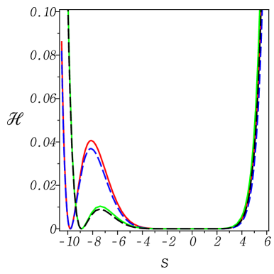
Figure 7: (Color online) ${\mathcal{H}}=h_{\scriptscriptstyle N}(s)\cdot 10^{-11}$ versus $s$, given in (6). Here we set $\Omega=M=1$ and $\omega_{d}=10$ as well as $N=5$. From top to bottom at $s=-7.5$, 1st) $h_{5,1}(s)\cdot 10^{-11}$: (red solid: $\gamma_{\mbox{\tiny o}}=0.2$ and $\kappa=0.2$) with a single multiple root, $s=-9.79840398$; 2nd) $h_{5,2}(s)\cdot 10^{-11}$: (blue dash: $\gamma_{\mbox{\tiny o}}=0.2$ and $\kappa=1$) with a multiple root, $s=-9.80006223$; 3rd) $h_{5,3}(s)\cdot 10^{-11}$: (green solid: $\gamma_{\mbox{\tiny o}}=1$ and $\kappa=0.2$) with a multiple root, $s=-8.89222703$; 4th) $h_{5,4}(s)\cdot 10^{-11}$: (black dash: $\gamma_{\mbox{\tiny o}}=1$ and $\kappa=1$) with a multiple root, $s=-8.90443052$. All the multiple roots have degeneracy $m=2$. We also have $h_{5,1}(0)=0.00000361\neq 0$; $h_{5,2}(0)=0.00005500$; $h_{5,3}(0)=0.00000361$; $h_{5,1}(0)=0.00005500$; in fact, $h_{\scriptscriptstyle N}(0)$ increases with increase of $N$. The numerical analysis of the exact expression of $h_{\scriptscriptstyle N}(s)$ reveals that there is no additional complex-valued multiple root of the above four functions. These properties of $h_{\scriptscriptstyle N}(s)$ are verified to be valid for many different choices of $(\gamma_{\mbox{\tiny o}},\kappa)$, and $N=3,4,\cdots,20$.

which is, in fact, valid for arbitrary values of the input parameters $(\Omega,\kappa,\omega_{d},\gamma_{\mbox{\tiny o}})$. Here the primed sum denoted by $\sum_{j}{}^{{}^{\prime}}\;[\cdots]$ means that if one of $z_{j}$’s is repeated, say, $z_{2{\scriptscriptstyle N}}=z_{2{\scriptscriptstyle N}+1}$ and so $h_{\scriptscriptstyle N}(s)=(s+z_{2{\scriptscriptstyle N}})^{2}\cdot f_{\scriptscriptstyle N}(s)$ where $f_{\scriptscriptstyle N}(s)=\prod_{j=0}^{2{\scriptscriptstyle N}-1}(s+z_{j})$ and $h_{\scriptscriptstyle N}^{\prime}(-z_{2{\scriptscriptstyle N}})=0$, then it is needed to consider this primed sum split into two parts such as $\sum_{j=0}^{2{\scriptscriptstyle N}-1}\,[\cdots]\,+\,\Lambda(2N,2N+1)$, where $h_{\scriptscriptstyle N}^{\prime}(-z_{j})=(-z_{j}+z_{2{\scriptscriptstyle N}})^{2}\cdot f_{\scriptscriptstyle N}^{\prime}(-z_{j})\neq 0$; the extra part denoted by $\Lambda(2N,2N+1)$ is contributed solely by the multiple root, $s=-z_{2{\scriptscriptstyle N}}$ [cf. (b)-(c)]. Fig. 7 plots the typical behaviors of $h_{\scriptscriptstyle N}(s)$. We also point out that the expression of heat current in (6), valid for $N\geq 3$, corresponds to the heat current ${\mathcal{J}}_{{\mbox{\tiny in}}}^{(2)}$ given in (5); note, however, that the denominator of each summand is here given by $h_{\scriptscriptstyle N}^{\prime}(-z_{j})\cdot h_{\scriptscriptstyle N}(z_{j})$ whereas it is in form of $h_{1}^{\prime}(-z_{j})\cdot h_{1}(z_{j})$ for $N=2$.

To simplify the expression in (6), we substitute (18) into this and then apply the same technique as for $N=1,2$. Then we can straightforwardly obtain the exact closed expression

$${\mathcal{J}}_{{\mbox{\tiny in}}}^{({\scriptscriptstyle N})}\,=\,-\frac{\kappa^{2}\gamma_{\mbox{\tiny o}}}{M^{2}}\,\left(\mbox{\={I}}_{\scriptscriptstyle N}\right)\cdot\left(\frac{1}{\beta_{1}}-\frac{1}{\beta_{\scriptscriptstyle N}}\right)\,+\,\frac{2\,\hbar\omega_{d}^{4}\,\gamma_{\mbox{\tiny o}}^{2}}{\pi}\,\times$$

$$\left(\frac{\kappa}{M}\right)^{2{\scriptscriptstyle N}-2}\;\sideset{}{{}^{\prime}}{\sum}_{j=0}^{2N+1}\,\frac{z_{j}^{3}\cdot\{\psi_{{\scriptscriptstyle\beta_{1}}}(z_{j})-\psi_{{\scriptscriptstyle\beta_{\scriptscriptstyle N}}}(z_{j})\}}{h_{\scriptscriptstyle N}^{\prime}(-z_{j})\cdot h_{\scriptscriptstyle N}(z_{j})}\,,$$ (45)

where

$$\left(\mbox{\={I}}_{\scriptscriptstyle N}\right)\,:=\,2\,\omega_{d}^{4}\,\gamma_{\mbox{\tiny o}}\,\left(\frac{\kappa}{M}\right)^{2{\scriptscriptstyle N}-4}\;\sideset{}{{}^{\prime}}{\sum}_{j}^{2N+1}\,\frac{-z_{j}^{2}}{h_{\scriptscriptstyle N}^{\prime}(-z_{j})\cdot h_{\scriptscriptstyle N}(z_{j})}\,;$$ (6a)

note that this is in the unit of $1/(\mbox{frequency})^{4}$ as is the case for $(\mbox{\={I}}_{2})$ given in (31a). Here we also employed the sum rule given by $\sum_{j}{}^{{}^{\prime}}\;z_{j}^{n}/\{h_{\scriptscriptstyle N}^{\prime}(-z_{j})\cdot h_{\scriptscriptstyle N}(z_{j})\}=0$ for $n$ odd (cf. Appendix E). If $z_{2{\scriptscriptstyle N}}=z_{2{\scriptscriptstyle N}+1}$, then the heat current ${\mathcal{J}}_{{\mbox{\tiny in}}}^{({\scriptscriptstyle N})}$ contains the terms contributed solely by this multiple root, explicitly given by ${\mathcal{J}}_{{\scriptscriptstyle\Lambda}}^{({\scriptscriptstyle N})}=J_{{\scriptscriptstyle\Lambda}}^{({\scriptscriptstyle N})}(\beta_{1})-J_{{\scriptscriptstyle\Lambda}}^{({\scriptscriptstyle N})}(\beta_{{\scriptscriptstyle N}})$, where

$$J_{{\scriptscriptstyle\Lambda}}^{({\scriptscriptstyle N})}(\beta_{\mu})\,=\,\frac{\hbar\,\omega_{d}^{4}\,\gamma_{\mbox{\tiny o}}^{2}\,(\kappa/M)^{2{\scriptscriptstyle N}-2}}{2\pi\cdot f_{\scriptscriptstyle N}(-z_{2{\scriptscriptstyle N}})\cdot f_{\scriptscriptstyle N}(z_{2{\scriptscriptstyle N}})\cdot z_{2{\scriptscriptstyle N}}}\,\times\,\Xi_{{\scriptscriptstyle\Lambda}}^{({\scriptscriptstyle N})}(\beta_{\mu})\,.$$ (6b)

Here $\mu=1,N$, and $f_{\scriptscriptstyle N}(-z_{2{\scriptscriptstyle N}})=h_{\scriptscriptstyle N}^{\prime\prime}(-z_{2{\scriptscriptstyle N}})/2$, as well as

$$\Xi_{{\scriptscriptstyle\Lambda}}^{({\scriptscriptstyle N})}(\beta_{\mu})\;=\;\frac{\omega_{\mu}}{2}\,-\,\frac{z_{2{\scriptscriptstyle N}}^{2}}{\omega_{\mu}}\cdot\psi_{{\scriptscriptstyle\beta_{\mu}}}^{(1)}(z_{2{\scriptscriptstyle N}})\,+$$

$$\frac{1}{\omega_{d}}\,\left(1\,+\,\sum_{j=0}^{2N-1}\frac{z_{2{\scriptscriptstyle N}}^{2}}{z_{j}^{2}\,-\,z_{2{\scriptscriptstyle N}}^{2}}\right)\,\times$$ (6c)

$$\left[\omega_{\mu}\,(z_{2{\scriptscriptstyle N}}\,-\,\omega_{d})\,-\,2\,z_{2{\scriptscriptstyle N}}\,\omega_{d}\,\{\psi_{{\scriptscriptstyle\beta_{\mu}}}(z_{2{\scriptscriptstyle N}})\,-\,\psi_{{\scriptscriptstyle\beta_{\mu}}}(\omega_{d})\}\right]\,,$$

where $\omega_{\mu}=2\pi/\beta_{\mu}\hbar$, and the trigamma function
$\psi_{{\scriptscriptstyle\beta_{\mu}}}^{(1)}(z_{2{\scriptscriptstyle N}})=\psi^{(1)}(z_{2{\scriptscriptstyle N}}/\omega_{\mu})$. If one of $z_{j}$’s is repeated over than twice, we can straightforwardly generalize the result given in (c) with the help of (67) and (71)-(72) ILK13 . It is also worthwhile to mention that the compact expression given in (6) can be rewritten in terms of the input parameters $(\Omega,\kappa,\omega_{d},\gamma_{\mbox{\tiny o}})$ with the aid of all coefficients of $h_{\scriptscriptstyle N}(s)$ explicitly given in (D) and their symmetric properties like given in (4) used for $N=1,2$; the resultant expression will, however, be highly complicated even for $N=3$. Eq. (6) is, in fact, the central result of this paper.

Next we consider the semiclassical behavior of the heat current ${\mathcal{J}}_{{\mbox{\tiny in}}}^{({\scriptscriptstyle N})}$. To do so, we expand the digamma function and its derivative given in (6)-(c) [cf. Appendix B], which will, in the semiclassical limit of $\beta_{\mu}\hbar\to 0$, give rise to

$${\mathcal{J}}_{{\mbox{\tiny in}}}^{({\scriptscriptstyle N})}\,=\,{\mathcal{J}}_{{\mbox{\tiny cl}}}^{({\scriptscriptstyle N})}(\hbar^{0})\,+\,{\mathcal{J}}_{{\mbox{\tiny q2}}}^{({\scriptscriptstyle N})}(\hbar^{2})\,+\,{\mathcal{J}}_{{\mbox{\tiny q3}}}^{({\scriptscriptstyle N})}(\hbar^{3})\,+\,{\mathcal{O}}(\hbar^{4})\,.$$ (46)

Here the leading term is given by the classical heat current

$${\mathcal{J}}_{{\mbox{\tiny cl}}}^{({\scriptscriptstyle N})}(\hbar^{0})\,=\,\frac{\kappa^{2}\gamma_{\mbox{\tiny o}}}{M^{2}}\,\left(\mbox{\={I}}_{\scriptscriptstyle N}\right)\cdot\left(\frac{1}{\beta_{1}}\,-\,\frac{1}{\beta_{\scriptscriptstyle N}}\right)\,.$$ (47)

If $z_{2{\scriptscriptstyle N}}=z_{2{\scriptscriptstyle N}+1}$, then this classical value contains ${\mathcal{J}}_{{\scriptscriptstyle\Lambda},{\mbox{\tiny cl}}}^{({\scriptscriptstyle N})}=J_{{\scriptscriptstyle\Lambda},{\mbox{\tiny cl}}}^{({\scriptscriptstyle N})}(\beta_{1})-J_{{\scriptscriptstyle\Lambda},{\mbox{\tiny cl}}}^{({\scriptscriptstyle N})}(\beta_{\scriptscriptstyle N})$, where

$$J_{{\scriptscriptstyle\Lambda},{\mbox{\tiny cl}}}^{({\scriptscriptstyle N})}(\beta_{\mu})\,=\,\frac{-\omega_{d}^{3}\,\gamma_{\mbox{\tiny o}}^{2}\,(\kappa/M)^{2{\scriptscriptstyle N}-2}}{2\,\beta_{\mu}\cdot f_{\scriptscriptstyle N}(-z_{2{\scriptscriptstyle N}})\cdot f_{\scriptscriptstyle N}(z_{2{\scriptscriptstyle N}})\cdot z_{2{\scriptscriptstyle N}}}\,\times$$

$$\left\{\omega_{d}\,-\,6\,(z_{2{\scriptscriptstyle N}}\,-\,\omega_{d})\,\left(1\,+\,\sum_{j=0}^{2N-1}\frac{z_{2{\scriptscriptstyle N}}^{2}}{z_{j}^{2}\,-\,z_{2{\scriptscriptstyle N}}^{2}}\right)\right\}\,.$$ (47a)

The first quantum correction is given by

$${\mathcal{J}}_{{\mbox{\tiny q2}}}^{({\scriptscriptstyle N})}(\hbar^{2})\,=\,\frac{1}{6}\,\hbar^{2}\,\omega_{d}^{4}\,\gamma_{\mbox{\tiny o}}^{2}\,\left(\frac{\kappa}{M}\right)^{2{\scriptscriptstyle N}-2}\,\left(\beta_{1}\,-\,\beta_{\scriptscriptstyle N}\right)\,\times$$ (48)

$$\sideset{}{{}^{\prime}}{\sum}_{j}^{2N+1}\,\frac{z_{j}^{4}}{h_{\scriptscriptstyle N}^{\prime}(-z_{j})\cdot h_{\scriptscriptstyle N}(z_{j})}\,,$$

if necessary, with

$$J_{{\scriptscriptstyle\Lambda},{\mbox{\tiny q2}}}^{({\scriptscriptstyle N})}(\beta_{\mu})\,=\,\frac{-\hbar^{2}\,\omega_{d}^{4}\,\gamma_{\mbox{\tiny o}}^{2}\,(\kappa/M)^{2{\scriptscriptstyle N}-2}\;\beta_{\mu}}{24\,f_{\scriptscriptstyle N}(-z_{2{\scriptscriptstyle N}})\cdot f_{\scriptscriptstyle N}(z_{2{\scriptscriptstyle N}})}\,\times$$

$$\left\{z_{2{\scriptscriptstyle N}}\,+\,2\,(z_{2{\scriptscriptstyle N}}\,-\,\omega_{d})\,\left(1\,+\,\sum_{j=0}^{2N-1}\,\frac{z_{2{\scriptscriptstyle N}}^{2}}{z_{j}^{2}\,-\,z_{2{\scriptscriptstyle N}}^{2}}\right)\right\}\,.$$ (48a)

The next quantum correction in ${\mathcal{O}}(\hbar^{3})$ is non-vanishing only if $z_{2{\scriptscriptstyle N}}=z_{2{\scriptscriptstyle N}+1}$ in such a way that

$$J_{{\scriptscriptstyle\Lambda},{\mbox{\tiny q3}}}^{({\scriptscriptstyle N})}(\beta_{\mu})\,=\,\frac{2\,\zeta(3)\,\hbar^{3}\,\omega_{d}^{4}\,\gamma_{\mbox{\tiny o}}^{2}\,(\kappa/M)^{2{\scriptscriptstyle N}-2}\;\beta_{\mu}^{2}}{(2\pi)^{3}\,f_{\scriptscriptstyle N}(-z_{2{\scriptscriptstyle N}})\cdot f_{\scriptscriptstyle N}(z_{2{\scriptscriptstyle N}})}\,\times$$

$$\left\{z_{2{\scriptscriptstyle N}}^{2}\,+\,(z_{2{\scriptscriptstyle N}}^{2}\,-\,\omega_{d}^{2})\,\left(1\,+\,\sum_{j=0}^{2N-1}\,\frac{z_{2{\scriptscriptstyle N}}^{2}}{z_{j}^{2}\,-\,z_{2{\scriptscriptstyle N}}^{2}}\right)\right\}\,,$$ (49)

where the symbol $\zeta(n)$ denotes the Riemann zeta function. In fact, all higher-order quantum corrections in closed form will straightforwardly come out.

It is now interesting to directly compare the classical result given in (47) with Fourier’s law of heat conduction. This allows us to identify the classical heat conductivity $\kappa_{{\mbox{\tiny F}}}$ as $(N\,\kappa^{2}\gamma_{\mbox{\tiny o}}/M^{2})\cdot(\mbox{\={I}}_{\scriptscriptstyle N})$, which depends on chain length $N$ hence violating Fourier’s law already. From the same comparison of the quantum result given in (46)-(6), we can easily find the “effective” heat conductivity, which depends even on temperature due to the quantum-correction contributions. Therefore, we may argue that non-universal behaviors of the (effective) heat conductivity, especially in low-dimensional lattices lying in the low-temperature regime (not only the harmonic chain under our investigation, as briefly stated in Sect. 1), are ascribed by the non-classical contributions, as explicitly given in (48)-(6) for the harmonic chain, which are, in fact, not proportional to $T_{1}-T_{{\scriptscriptstyle N}}$ any longer.

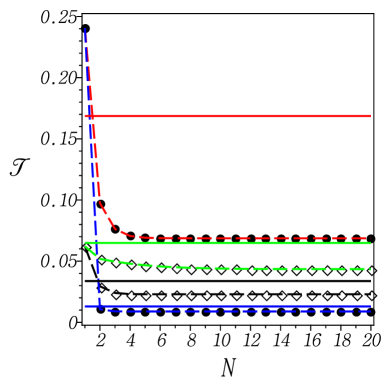
Figure 8: (Color online) Heat current ${\mathcal{J}}={\mathcal{J}}_{{\mbox{\tiny in}}}^{({\scriptscriptstyle N})}(T_{1},T_{\scriptscriptstyle N})$ versus chain length $N$, given in (6)-(c), in the low-temperature regime imposed by $T_{1}=1.1$ and $T_{\scriptscriptstyle N}=0.1$. Here we set $\hbar=k_{\mbox{\tiny B}}=M=\Omega=1$, and $\omega_{d}=10$. Dashed lines, from top to bottom at $N=20$, 1st: (red with solid circles: $\gamma_{\mbox{\tiny o}}=\kappa=1$); 2nd: (green with diamonds: $\gamma_{\mbox{\tiny o}}=0.2$ and $\kappa=1$); 3rd: (black with diamonds: $\gamma_{\mbox{\tiny o}}=\kappa=0.2$); 4th: (blue with solid circles: $\gamma_{\mbox{\tiny o}}=1$ and $\kappa=0.2$). In comparison, solid lines are inserted for ${\mathcal{J}}_{{\mbox{\tiny B-M}}}^{({\scriptscriptstyle N})}$ given in (51), from top to bottom, in the same order as for the dashed lines. As demonstrated, this represents a good approximation in the weak-coupling regime.

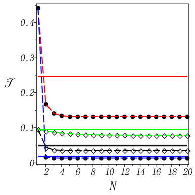
Figure 9: (Color online) The same plot as in Fig. 8, in the high-temperature regime imposed by $T_{1}=3$ and $T_{\scriptscriptstyle N}=2$.

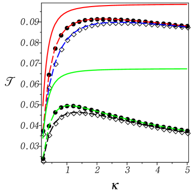
Figure 10: (Color online) Heat current ${\mathcal{J}}={\mathcal{J}}_{{\mbox{\tiny in}}}^{({\scriptscriptstyle N})}(T_{1},T_{\scriptscriptstyle N};\kappa)$ versus intra-coupling strength $\kappa$, given in (6)-(c). Here we set $\hbar=k_{\mbox{\tiny B}}=M=\Omega=1$, and $\omega_{d}=10$, as well as $\gamma_{\mbox{\tiny o}}=0.2$. Dashed lines, from top to bottom at $\kappa=1$, 1st: (red with solid circles: $N=3$ as well as $T_{1}=3$ and $T_{\scriptscriptstyle N}=2$, with its maximum at $\kappa=\kappa_{\mbox{\tiny R}}=2.2$); 2nd: (blue with diamonds: $N=6$ as well as $T_{1}=3$ and $T_{\scriptscriptstyle N}=2$, with $\kappa_{\mbox{\tiny R}}=2.8$); 3rd: (green with solid circles: $N=3$ as well as $T_{1}=1.1$ and $T_{\scriptscriptstyle N}=0.1$, with $\kappa_{\mbox{\tiny R}}=1$); 4th: (black with diamonds: $N=6$ as well as $T_{1}=1.1$ and $T_{\scriptscriptstyle N}=0.1$, with $\kappa_{\mbox{\tiny R}}=1.4$). This shape of the heat current with respect to the intra-coupling strength is verified to be true for different choices of the temperature range and all other input parameters. In comparison, two solid lines are inserted for ${\mathcal{J}}_{{\mbox{\tiny B-M}}}^{({\scriptscriptstyle N})}$ given in (51); the red upper for $T_{1}=3$ and $T_{\scriptscriptstyle N}=2$, asymptotically approaching $0.09862324$ with $\kappa\to\infty$, and the green lower for $T_{1}=1.1$ and $T_{\scriptscriptstyle N}=0.1$, approaching $0.06746888$ with $\kappa\to\infty$.

The behaviors of heat current ${\mathcal{J}}_{{\mbox{\tiny in}}}^{({\scriptscriptstyle N})}$ versus chain length $N$ are plotted in Figs. 8-10 for various input parameters. First, it turns out that in the weak-coupling regime imposed by $\kappa/M,\gamma_{\mbox{\tiny o}}^{2}\ll\Omega^{2}$, the low-magnitude heat currents are typically acquired, as expected from the results for $N=1,2$. They also reveal the almost $N$-independent behaviors (for $N\geq 2$). This can be understood from the forms of the matrix elements ${\mathcal{A}}_{11}(s)$ and ${\mathcal{A}}_{12}(s)$ in the weak-coupling limit; with the aid of $\sin N\phi=\sin\phi\cdot\cos(N-1)\phi+\cos\phi\cdot\sin(N-1)\phi$, we can exactly rewrite ${\mathcal{A}}_{11}(s)$ in (34) as

$$\frac{\delta\,-\,c\cdot\cos\phi\,-\,c\cdot\sin\phi\cdot\cot(N-1)\phi}{{\mathcal{A}}_{{\mbox{\tiny den}}}(s)}\,,$$ (50)

where

$${\mathcal{A}}_{{\mbox{\tiny den}}}(s)\,:=\,\delta^{2}\,-\,c^{2}\,+\,2c\cdot(c\,\cos\phi\,-\,\delta)\cdot\cos\phi\,+$$

$$2c\cdot(c\,\cos\phi\,-\,\delta)\cdot\sin\phi\cdot\cot(N-1)\phi\,,$$ (50a)

as well as $\cot(N-1)\phi=-i\coth(N-1)r$, expressed in terms of the real number $r=-i\phi>0$, with

$$\coth(N-1)r\,=\,\frac{2}{1\,-\,(e^{-r})^{2({\scriptscriptstyle N}-1)}}\,-\,1\,.$$ (50b)

In the weak-coupling limit leading to $|c|\ll b+2c$, Eqs. (36c) and (36d) allow us to easily have

$$e^{-r}\,=\,-\frac{1}{2c}\,H(s)\,=$$ (50c)

$$-\frac{c}{s^{2}\,+\,\Omega^{2}}\,-\,2\left(\frac{c}{s^{2}\,+\,\Omega^{2}}\right)^{2}\,+\,{\mathcal{O}}\left\{\left(\frac{c}{s^{2}\,+\,\Omega^{2}}\right)^{3}\right\}\,,$$

which gives rise to $\coth(N-1)r\to 1$ for $N$ large enough (a fairly good approximation even for $N=3$). Accordingly, the matrix element ${\mathcal{A}}_{11}(s)$ reduces to be
$N$-independent. Along the same line, we can do the same job for ${\mathcal{A}}_{12}(s),{\mathcal{A}}_{1{\scriptscriptstyle N}}(s)$ and ${\mathcal{A}}_{2{\scriptscriptstyle N}}(s)$, respectively. Consequently, the heat current ${\mathcal{J}}_{{\mbox{\tiny in}}}^{({\scriptscriptstyle N})}$ reduces to be
$N$-independent in this regime. In this context, it is also worthwhile to mention that this behavior of heat current is consistent to the result by Asadian et al. in BRI13 , which was obtained from the consideration of a harmonic chain restricted to the rotating wave approximation of the isolated chain $\hat{H}_{s}$ given in (1a) as well as to the Born-Markovian regime imposed by the weak-coupling and the Ohmic damping ($\omega_{d}\to\infty$). Their result for steady-state heat current can be rewritten in terms of our notation, i.e., with $V\to\kappa/2$ as well as $\Gamma_{1},\Gamma_{\scriptscriptstyle N}\to\gamma_{\mbox{\tiny o}}$ in their equation (25), as the $N$-independent expression

$${\mathcal{J}}_{{\mbox{\tiny B-M}}}^{({\scriptscriptstyle N})}\,=\,\frac{\kappa^{2}\gamma_{\mbox{\tiny o}}}{M^{2}}\,\left(\mbox{\={I}}_{\mbox{\tiny B-M}}\right)\cdot\hbar\,\Omega\,\left(\langle\hat{n}\rangle_{{\scriptscriptstyle\beta_{1}}}\,-\,\langle\hat{n}\rangle_{\scriptscriptstyle\beta_{\scriptscriptstyle N}}\right)\,,$$ (51)

where $(\mbox{\={I}}_{\mbox{\tiny B-M}}):=(1/2)\,\{(\kappa/M)^{2}\,+\,(\Omega\,\gamma_{\mbox{\tiny o}})^{2}\}^{-1}$, and the average excitation number $\langle\hat{n}\rangle_{{\scriptscriptstyle\beta_{\mu}}}=1/(e^{{\scriptscriptstyle\beta_{\mu}}\hbar\Omega}\,-\,1)$. In Figs. 8-10, this approximation is compared with our exact result denoted by ${\mathcal{J}}_{{\mbox{\tiny in}}}^{({\scriptscriptstyle N})}$. It is then shown that this may be a good approximation in the weak-coupling regime, as expected, whereas it is not case beyond the weak-coupling regime.

Next we pay attention to the above behavior of heat current beyond the weak-coupling regime, which has so far not been systematically explored. As demonstrated in the figures, the heat current increases with increase of the intra-coupling strength $\kappa$ for a given chain-bath coupling strength characterized by the imposed damping parameter $\gamma_{\mbox{\tiny o}}$, and reaches its maximum value at some specific coupling strength $\kappa_{\mbox{\tiny R}}$ “resonant” to the chain-bath coupling strength. With further increase of the intra-coupling strength, the heat current decreases very slowly, whereas this behavior cannot be found from the Born-Markovian result given in (51). Also, the heat current typically behaves in such a way that its magnitude is at the maximum with $N=1$, and then gradually decreases with increase of chain length $N$, being in fact almost $N$-independent in the range of $N$ large enough. This may already be qualitatively underwood from the behavior of $\coth(N-1)r$ given in (50) with respect to $N$. As a result, Fourier’s law proves violated also in this regime.

7 Conclusion

In summary, we derived an exact closed expression of the steady-state heat current through a chain of quantum Brownian oscillators coupled to two separate baths. It was obtained, without any approximation indeed, for arbitrary coupling strengths both in the intra-couplings between two nearest-neighboring chain elements and in the chain-baths couplings, as well as in the Drude-Ullersma damping model in order to look at the behavior of this heat current beyond the Born-Markovian regime. Then we systematically observed that in the weak-coupling regime, the heat current with its low-magnitude simply reduces to be almost independent of the chain length while in the regime beyond the weak-coupling, the magnitude of heat current can be raised up by appropriate manipulation of the chain-baths coupling strengths and the intra-chain coupling strengths as control parameters; in fact, the largest currents result if both couplings are “resonant” in a sense of comparable strengths (cf. Figs. 8-9).

As a result, this rigorous study carried out from the fundamental side contains the previous results of heat transport in the same type of harmonic chains, as cited in Sect. 1, as the corresponding limiting cases. By doing so, we could also explore the relevance between the coupling strengths as input parameters and the magnitude of the output heat-current, which may be considered a fundamental issue for building a quantum thermodynamic engine with high power. We believe that our finding will provide a useful starting point for the analytical approach to the steady-state heat current through a more general type of quantum Brownian chains beyond the weak-coupling regime.

Appendix A Derivation of correlation function in Eq. (3a)

To derive a closed form of the correlation function in (3), we first employ the identity

$$\coth\left(\frac{\beta\hbar\omega}{2}\right)\,=\,\frac{2}{\beta\hbar\omega}\left(1+2\sum_{n=1}^{\infty}\frac{\omega^{2}}{\omega^{2}+\nu_{n}^{2}}\right)\,,$$ (52)

where the so-called Matsubara frequencies $\nu_{n}=2\pi n/(\beta\hbar)$ WEI08 . Substituting (52) into (3) and then applying the integral identities GRA07

$$\int_{0}^{\infty}dy\,\frac{\cos(ay)}{y^{2}+b^{2}} = \frac{\pi}{2}\,\frac{e^{-ab}}{b}\;,$$

$$\int_{0}^{\infty}\frac{dy\,\cos(ay)}{(y^{2}+b^{2})\,(y^{2}+c^{2})} = \frac{\pi}{2}\,\frac{b\,e^{-ac}-c\,e^{-ab}}{bc\,(b^{2}-c^{2})}\,,$$ (53)

we can straightforwardly obtain

$$\int_{0}^{\infty}d\omega\,\frac{\omega}{\omega^{2}+\omega_{d}^{2}}\,\coth\left(\frac{\beta\hbar\omega}{2}\right)\,\cos\{\omega(t-t^{\prime})\}$$

$$= \frac{\pi}{\beta\hbar\omega_{d}}\,e^{-\omega_{d}\,|t-t^{\prime}|}\,+\,\frac{2\pi}{\beta\hbar}\sum_{n=1}^{\infty}\frac{\nu_{n}\,e^{-\nu_{n}\,|t-t^{\prime}|}-\omega_{d}\,e^{-\omega_{d}\,|t-t^{\prime}|}}{\nu_{n}^{2}-\omega_{d}^{2}}\,.$$

We next apply to this expression both sum rules

$$\sum_{n=1}^{\infty}\frac{1}{n^{2}-y^{2}}\,=\,\frac{1-\pi y\,\cot(\pi y)}{2y^{2}}$$ (55)

and

$$\sum_{n=1}^{\infty}\frac{2n\,e^{-an}}{n^{2}-y^{2}}\,=\,\Phi(e^{-a},1,y)+\Phi(e^{-a},1,-y)$$ (56)

expressed in terms of the Lerch function GRA07

$$\Phi(z,s,v)\,=\,\sum_{n=0}^{\infty}\frac{z^{n}}{(n+v)^{s}}\,,$$ (57)

which finally gives rise to the closed expression in (3a).

Appendix B Derivation of Eqs. (17)-(a)

We first substitute (13) into (16), which immediately yields

$$\left\langle\left\{\hat{P}_{1}(t)\,,\,\xi_{b_{1}}(t)\right\}_{+}\right\rangle^{({\mbox{\tiny ss}})}\,=$$

$$2M\lim_{t\to\infty}\int_{0}^{t}d\tau\,\left\{\frac{\partial}{\partial t}\chi_{d}(t-\tau)\right\}\,K_{1}^{(d)}(t-\tau)\,.$$ (58)

Here the bath correlation function is explicitly given by

$$K_{\mu}^{(d)}(t-\tau) = \frac{\hbar\omega_{d}^{2}\,M\gamma_{\mbox{\tiny o}}}{2\pi}\,\left\{\pi\,\cot\left(\frac{\beta_{\mu}\hbar\omega_{d}}{2}\right)\,e^{-\omega_{d}\,|t-\tau|}\,+\right.$$ (59)

$$\left.\sum_{n=0}^{\infty}\,\frac{2\,n\cdot e^{-n\,\omega_{\mu}\,|t-\tau|}}{(n+\omega_{d}/\omega_{\mu})\cdot(n-\omega_{d}/\omega_{\mu})}\right\}$$

[cf. (57)]. We can easily evaluate the integral in (B) explicitly, which leads to

$$\left\langle\left\{\hat{P}_{1}(t)\,,\,\xi_{b_{1}}(t)\right\}_{+}\right\rangle^{({\mbox{\tiny ss}})}\,=\,\frac{\hbar\omega_{d}^{2}\,\gamma_{\mbox{\tiny o}}\,M\cdot{\mathcal{Y}}_{{\scriptscriptstyle\beta_{1}}}}{\pi\,(z_{0}-z_{1})(z_{1}-z_{2})(z_{2}-z_{0})}\,.$$ (60)

Here

$${\mathcal{Y}}_{{\scriptscriptstyle\beta_{1}}} = \pi\,\cot\left(\frac{\beta_{1}\hbar\omega_{d}}{2}\right)\cdot Y(\omega_{d})\,+$$ (61)

$$\sum_{n=0}^{\infty}\left(\frac{1}{n+\omega_{d}/\omega_{1}}\,+\,\frac{1}{n-\omega_{d}/\omega_{1}}\right)\cdot Y\left(n\,\omega_{1}\right)\,,$$

where

$$Y(\omega)\,=\,\sum_{\underline{j}=0}^{2}\frac{(z_{\underline{j+1}}^{2}-z_{\underline{j+2}}^{2})\,z_{\underline{j}}}{\omega+z_{\underline{j}}}\,.$$ (62)

By means of the identity of the digamma function ABS74

$$\sum_{n=0}^{\infty}\frac{1}{(n+a)\,(n+b)}\,=\,\frac{\psi(a)-\psi(b)}{a-b}\,,$$ (63)

we can easily rewrite the summation in (61) as

$$-\left[Y(\omega_{d})\cdot\sum_{\underline{j}=0}^{2}\left\{\psi\left(-\frac{\beta_{1}\hbar\omega_{d}}{2\pi}\right)-\psi\left(\frac{\beta_{1}\hbar z_{\underline{j}}}{2\pi}\right)\right\}\right]\,-\,\left[\omega_{d}\to-\omega_{d}\right]\,.$$ (64)

Substituting now the expression in (61) into (60) and subsequently into (16), we can finally arrive at the result given in (17).

Next let us derive the expression of heat current given in (4) in terms of the input parameters $(\Omega,\omega_{d},\gamma_{\mbox{\tiny o}})$ only, expanded in the semiclassical limit. To do so, we first plug into (17) the expansions given by
$\cot(y)=\sum_{n=0}^{\infty}\,(-1)^{n}\,\{2^{2n}/(2n)!\}\,B_{2n}\,y^{2n-1}$ for $0<|y|<\pi$ and $\psi(y)=-1/y-\gamma_{e}+\sum_{n=1}^{\infty}\,(-1)^{n+1}\,\zeta(n+1)\,y^{n}$; here the Bernoulli numbers $B_{2n}$, the Euler constant $\gamma_{e}=0.5772\cdots$, and the Riemann zeta function $\zeta(n+1)$, as well as $B_{2n}=2\,(-1)^{n-1}\{(2n)!/(2\pi)^{2n}\}\,\zeta(2n)$ GRA07 . After some steps of algebraic manipulation, this gives rise to

$${\mathcal{J}}_{{\mbox{\tiny in}}}^{(1)} = {\mathcal{J}}_{{\mbox{\tiny cl}}}^{(1)}(\hbar^{0})\,+\,{\mathcal{J}}_{{\mbox{\tiny q1}}}^{(1)}(\hbar^{1})\,+\,{\mathcal{J}}_{{\mbox{\tiny q2}}}^{(1)}(\hbar^{2})\,+\,{\mathcal{J}}_{{\mbox{\tiny q3}}}^{(1)}(\hbar^{3})\,+$$ (65)

$${\mathcal{J}}_{{\mbox{\tiny q4}}}^{(1)}(\hbar^{4})\,+\,{\mathcal{J}}_{{\mbox{\tiny q5}}}^{(1)}(\hbar^{5})\,+\,{\mathcal{O}}(\hbar^{6})\,.$$

Here we have the leading term

$${\mathcal{J}}_{{\mbox{\tiny cl}}}^{(1)}(\hbar^{0}) = \frac{\gamma_{\mbox{\tiny o}}\,\omega_{d}}{2}\left(\frac{1}{\beta_{1}}-\frac{1}{\beta_{1^{\prime}}}\right)\,\times$$ (66)

$$\sum_{\underline{j}=0}^{2}\frac{z_{\underline{j}}\,(z_{\underline{j}}-\omega_{d})}{(z_{\underline{j}}-z_{\underline{j+1}})(z_{\underline{j}}-z_{\underline{j+2}})(z_{\underline{j}}+\omega_{d})}\,.$$

To evaluate this summation explicitly, we take into account the technique of partial fraction for two polynomials $P(s)$ and $Q(s)$ with $\mbox{deg}\,Q(s)<\mbox{deg}\,P(s)=n$, where $P(s)=(s-b_{1})(s-b_{2})\cdots(s-b_{n})$ with $b_{j}\neq b_{k}$ for $j\neq k$. This is explicitly given by COH07

$$\bar{f}(s)\;:=\;\frac{Q(s)}{P(s)}\;=\;\sum_{\nu=1}^{n}\frac{Q(b_{\nu})}{P^{\prime}(b_{\nu})\cdot(s-b_{\nu})}\,.$$ (67)

Applying this relation, the summation in (66) easily reduces to

$$\left.\frac{s\,\left(s+\omega_{d}\right)}{\left(s+z_{0}\right)\left(s+z_{1}\right)\left(s+z_{2}\right)}\right|_{s\to\omega_{d}}\,,$$ (68)

which allows us to have the classical result in (a). Here we also used the relations in (4). Next, we consider the quantum corrections

$${\mathcal{J}}_{{\mbox{\tiny q2}}}^{(1)}(\hbar^{2}) = \frac{\hbar^{2}\omega_{d}^{2}\,\gamma_{\mbox{\tiny o}}}{24}\,\left(\beta_{1}-\beta_{1^{\prime}}\right)\,\times$$

$$\sum_{\underline{j}=0}^{2}\frac{z_{\underline{j}}^{2}\,(z_{\underline{j}}-\omega_{d})}{(z_{\underline{j}}-z_{\underline{j+1}})(z_{\underline{j}}-z_{\underline{j+2}})(z_{\underline{j}}+\omega_{d})}$$

$${\mathcal{J}}_{{\mbox{\tiny q4}}}^{(1)}(\hbar^{4}) = \frac{\hbar^{4}\omega_{d}^{2}\,\gamma_{\mbox{\tiny o}}}{2^{5}\cdot 3^{2}\cdot 5}\,\left(\beta_{1}^{3}-\beta_{1^{\prime}}^{3}\right)\,\times$$

$$\sum_{\underline{j}=0}^{2}\frac{z_{\underline{j}}^{2}\,(z_{\underline{j}}^{3}-\omega_{d}^{3})}{(z_{\underline{j}}-z_{\underline{j+1}})(z_{\underline{j}}-z_{\underline{j+2}})(z_{\underline{j}}+\omega_{d})}\,.$$

Here we used $\zeta(2)=\pi^{2}/6$ and $\zeta(4)=\pi^{4}/90$. Applying again (67) to these two summations and then evaluating them at $s=\omega_{d}$, respectively, we can finally arrive at the result in (4). In fact, every quantum correction with the odd-degree $\hbar$-power in (65) is shown to vanish indeed by applying the same technique. Along the same line, we can also derive the expression of heat current given in (4), valid in the low-temperature limit, by plugging into (4) the asymptotic expansion given by $\psi(y)=\ln y-1/2y-\sum_{n=1}^{\infty}\,(B_{2n}/2n)/y^{2n}$ ABS74 .

Finally we point out that if one of the roots $b_{\nu}$ is repeated $m$ times in (67), then the expansion for $\bar{f}(s)$ contains the terms of form

$$\frac{\lambda_{1}}{s-b_{\nu}}\,+\,\frac{\lambda_{2}}{(s-b_{\nu})^{2}}\,+\,\cdots\,+\,\frac{\lambda_{m}}{(s-b_{\nu})^{m}}\,,$$ (71)

where

$$\lambda_{m-r}\,=\,\lim_{s\to b_{\nu}}\,\left[\frac{1}{r!}\,\left(\frac{d}{ds}\right)^{r}\left\{(s-b_{\nu})^{m}\cdot\bar{f}(s)\right\}\right]\,.$$ (72)

This will be used in Sect. 6.

Appendix C Evaluation of Eqs. (27)-(5)

We consider the double integral given in (27)

$$(\mbox{I}_{2})\,:=\,\lim_{t\to\infty}\,\int_{0}^{t}d\tau\int_{0}^{t}d\tau^{\prime}\,\chi_{1}(t-\tau)\cdot\partial_{t}\{\chi_{2}(t-\tau^{\prime})\}\cdot K_{\mu}^{(d)}(\tau-\tau^{\prime})\,.$$ (73)

We substitute (12a) and (59) into this. In doing so, let $\chi_{d}(t)\to\chi_{1}(t)$ expressed in terms of $\bar{z}_{1,j}$’s, and $\chi_{d}(t)\to\chi_{2}(t)$ expressed in terms of $\bar{z}_{2,j}$’s. Then it turns out that

$$(\mbox{I}_{2})=-\frac{\hbar\omega_{d}^{2}\,\gamma_{\mbox{\tiny o}}}{2\pi M}\,\times$$

$$\frac{\sum_{\underline{j},\underline{k}=0}^{2}\,(\bar{z}_{1,\underline{j+1}}^{2}-\bar{z}_{1,\underline{{j+2}}}^{2})\,(\bar{z}_{2,\underline{k+1}}^{2}-\bar{z}_{2,\underline{{k+2}}}^{2})\,\bar{z}_{2,\underline{{k}}}}{\{(\bar{z}_{1,0}-\bar{z}_{1,1})\,(\bar{z}_{1,1}-\bar{z}_{1,2})\,(\bar{z}_{1,2}-\bar{z}_{1,0})\}\cdot\{(\bar{z}_{1,l}\to\bar{z}_{2,l})\}}\,\times$$

$$\left\{\pi\,\cot\left(\frac{\beta_{\mu}\hbar\omega_{d}}{2}\right)\cdot(\mbox{I}_{2,1})_{\omega_{d}}\,+\right.$$

$$\left.\sum_{n=0}^{\infty}\,\frac{2\,n}{(n+\omega_{d}/\omega_{\mu})\cdot(n-\omega_{d}/\omega_{\mu})}\cdot(\mbox{I}_{2,1})_{n\omega_{\mu}}\right\}\,,$$ (74)

where $l=0,1,2$, and

$$(\mbox{I}_{2,1})_{\alpha} := \lim_{t\to\infty}\,\int_{0}^{t}d\tau\,e^{-\bar{z}_{1,j}\,(t-\tau)}\int_{0}^{t}d\tau^{\prime}\,e^{-\bar{z}_{2,k}\,(t-\tau^{\prime})}\,e^{-\alpha\,|\tau-\tau^{\prime}|}$$ (75)

$$= \frac{1}{\bar{z}_{1,j}+\bar{z}_{2,k}}\left(\frac{1}{\bar{z}_{1,j}+\alpha}\,+\,\frac{1}{\bar{z}_{2,k}+\alpha}\right)\,.$$

Here we also used the integral identity given in (15).

Next we consider

$$(\mbox{II}_{2})\,:=\,\lim_{t\to\infty}\,\int_{0}^{t}d\tau\int_{0}^{t}d\tau^{\prime}\,\partial_{t}\{\chi_{1}(t-\tau)\}\cdot\chi_{2}(t-\tau^{\prime})\cdot K_{\mu}^{(d)}(\tau-\tau^{\prime})\,.$$ (76)

Along the same line, this reduces to the expression given in (C) but with exchange of $\bar{z}_{1,\underline{{j}}}$ and $\bar{z}_{2,\underline{{k}}}$. Noting $\chi_{1}(0)=\chi_{2}(0)=0$ from (12a), we can first find that $(\mbox{I}_{2})+(\mbox{II}_{2})$ vanishes indeed, and so does Eq. (27). Next, $(\mbox{I}_{2})-(\mbox{II}_{2})$ gives rise to an explicit evaluation of the integral in (5) and subsequently the exact result in (5) expressed in terms of $\{z_{\underline{j}}|\,z_{\underline{j}}=\bar{z}_{1,\underline{j}}\}$ and $\{z_{\underline{j}}^{\prime}|\,z_{\underline{j}}^{\prime}=\bar{z}_{2,\underline{j}}\}$.

Appendix D Mathematical supplements for Eq. (6)

First, let us acquire an explicit expression of $\mbox{den}(s;N)$ which leads to the polynomial $h_{\scriptscriptstyle N}(s)=\mbox{den}(s;N)\cdot(s+\omega_{d})^{2}$. To do so, we rewrite Eq. (36c) as $F_{\scriptscriptstyle N}(s)=F_{1}(s)\cdot T_{\scriptscriptstyle N}(s)$, where

$$T_{\scriptscriptstyle N}(s) = \sum_{\nu=0}^{N-1}\,\{G(s)\}^{{\scriptscriptstyle N}-1-\nu}\cdot\{H(s)\}^{\nu}$$ (77)

$$= \sum_{j=0}^{\infty}\,\binom{N}{2j+1}\cdot b^{{\scriptscriptstyle N}-2j-1}\cdot\left(b^{2}-4\,c^{2}\right)^{j}\,.$$

With the aid of (36a)-(36b), we can then find that

$${\mathcal{A}}_{11}(s)=\frac{2^{1-{\scriptscriptstyle N}}}{\mbox{den}(s;N)}\,\left[T_{\scriptscriptstyle N}(s)\,+\,2\,\{s\,\bar{\gamma}(s)+c\}\cdot T_{{\scriptscriptstyle N}-1}(s)\right]$$ (78a)

$${\mathcal{A}}_{12}(s)=\frac{2^{2-{\scriptscriptstyle N}}\,(-c)}{\mbox{den}(s;N)}\,\left[T_{{\scriptscriptstyle N}-1}(s)\,+\,2\,\{s\,\bar{\gamma}(s)+c\}\cdot T_{{\scriptscriptstyle N}-2}(s)\right]$$ (78b)

$${\mathcal{A}}_{1{\scriptscriptstyle N}}(s)=\frac{(-c)^{{\scriptscriptstyle N}-1}}{\mbox{den}(s;N)}\;,\;{\mathcal{A}}_{2{\scriptscriptstyle N}}(s)=\frac{a\,(-c)^{{\scriptscriptstyle N}-2}}{\mbox{den}(s;N)}\,.$$ (78c)

Substituting (77) into (36b) and then applying Pascal’s rule $\binom{N}{k}=\binom{N-1}{k}+\binom{N-1}{k-1}$, we can finally arrive, after some algebraic manipulations, at the expression

$$\mbox{den}(s;N)\,=\,2^{1-{\scriptscriptstyle N}}\sum_{j,k,n=0}^{\infty}\binom{N-2j-2}{k}\,\left\{\binom{N-1}{2j+1}\,\times\right.$$

$$\left[d^{2}\,+\,2\,\{x+(-c)\}\,d\,+\,2x^{2}\right]\,+\,\binom{N-1}{2j}\,\times$$

$$\left.\left[d^{2}\,+\,2\,\{x+(-c)\}\,d\,+\,4\,(-c)\,x\right]\right\}\,\binom{j}{n}\times$$

$$2^{k+2n}\cdot d^{{\scriptscriptstyle N}-k-n-2}\cdot(-c)^{k+n}\,,$$ (79)

where $x(s):=s\,\bar{\gamma}_{d}(s)$ and $d(s):=s^{2}+\Omega^{2}$. From this, all coefficients of $\mbox{den}(s;N)$ can exactly be determined, which are non-negative, as shown; e.g., the highest $s$-power term is given by $s^{2{\scriptscriptstyle N}+2}/(s+\omega_{d})^{2}$ and the second highest $s$-power term is $2\,\omega_{d}\,s^{2\scriptscriptstyle N+1}/(s+\omega_{d})^{2}$. Substituting (D) into (78a)-(78c), we can get the explicit expressions in (6).

Next, we let us prove that $\mbox{Re}(z_{j})>0$ for all $z_{j}$’s satisfying $h_{\scriptscriptstyle N}(-z_{j})=0$, which is needed for applying the final value theorem of the Laplace transform. Due to the non-negativeness of all coefficients given in (D), it suffices to prove that $\mbox{den}(s;N)\neq 0$ for any purely imaginary number $s=ir$, where $r\in{\mathbb{R}}$. We assume that $\mbox{den}(ir;N)=0$, though. Then, its conjugate number $s=-ir$ should also satisfy the equality, $\mbox{den}(-ir;N)\stackrel{{\scriptstyle!}}{{=}}0$. By applying these two equality conditions to (34b) simultaneously, we can obtain both

$$c\cdot\sin N\phi=\left(c+\frac{r^{2}\,\gamma_{\mbox{\tiny o}}\,\omega_{d}}{r^{2}+\omega_{d}^{2}}\right)\cdot\sin(N-1)\phi$$

$$c\,\left(c+\frac{r^{2}\,\gamma_{\mbox{\tiny o}}\,\omega_{d}}{r^{2}+\omega_{d}^{2}}\right)\cdot\sin(N+1)\phi$$

$$= \delta\,\left\{2\,\left(c+\frac{r^{2}\,\gamma_{\mbox{\tiny o}}\,\omega_{d}}{r^{2}+\omega_{d}^{2}}\right)-\delta\right\}\cdot\sin N\phi\,.$$ (80b)

From this, we notice that $\sin N\phi\neq 0$ if $\sin\phi\neq 0$. Combining (80) and (80b) to eliminate the sine functions therein, we can easily acquire

$$\{(\gamma_{\mbox{\tiny o}}\,\omega_{d}+c)^{2}+c^{2}\}\,X^{2}\,+\,\omega_{d}^{2}\,\{(\gamma_{\mbox{\tiny o}}\,\omega_{d}+c)^{2}+3\,c^{2}\}\,X\,+\,2\,c^{2}\,\omega_{d}^{4}\,=\,0\,,$$ (81)

where $X:=r^{2}>0$. Then we see that each root $X_{q}$ of this quadratic equation would be required to meet the condition $\mbox{Re}(X_{q})<0$, which, however, contradicts itself. Consequently, we cannot have any numbers $z_{j}$’s being purely imaginary. It is, however, nontrivial indeed to extract all individual roots $(-z_{j})$’s of the polynomial $h_{\scriptscriptstyle N}(s)$ expressed explicitly in terms of the parameters $(\Omega,\kappa,\omega_{d},\gamma_{\mbox{\tiny o}})$, even for $N=3$ when we need to deal with the $8$th-degree polynomial $h_{3}(s)$.

Appendix E Evaluation of Eqs. (6)-(6)

To evaluate the integral in (6) explicitly, we first consider the double integral

$$(\mbox{I}_{\scriptscriptstyle N})_{\alpha}\,:=\,\lim_{t\to\infty}\,\int_{0}^{t}d\tau\,f(t-\tau)\int_{0}^{t}d\tau^{\prime}\,g(t-\tau^{\prime})\cdot e^{-\alpha\,|\tau-\tau^{\prime}|}\,,$$ (82)

where $f(t)=\dot{A}_{11}(t)$ and $g(t)=A_{21}(t)$. By applying the technique in (75) used for $N=2$, we can transform (82) into

$$(\mbox{I}_{{\scriptscriptstyle N}})_{\alpha}\,=\,{\mathcal{L}}\left\{\int_{0}^{t}d\tau\,\left[f(t)\cdot g(\tau)\,+\,g(t)\cdot f(\tau)\right]\,e^{\alpha\tau}\right\}(\alpha)\,.$$ (83)

Let $\bar{f}(s)={\mathcal{L}}\{f(t)\}(s)$ and $\bar{g}(s)={\mathcal{L}}\{g(t)\}(s)$. Now we consider the product rule, which reads as ${\mathcal{L}}\{f_{1}(t)\,f_{2}(t)\}(s)=(1/2\pi i)\int_{c_{1}-i\infty}^{c_{1}+i\infty}du\,\bar{f}_{1}(u)\,\bar{f}_{2}(s-u)$ COH07 ; here the integration is carried out along the vertical line, $\mbox{Re}(u)=c_{1}$ that lies entirely within the region of convergence of $\bar{f}_{1}(u)$. Then we can easily rewrite (83) as

$$(\mbox{I}_{{\scriptscriptstyle N}})_{\alpha}\,=\,\int_{c_{1}-i\infty}^{c_{1}+i\infty}\frac{du}{u-\alpha}\,\left\{\bar{f}(u)\,\bar{g}(-u)\,+\,\bar{g}(u)\,\bar{f}(-u)\right\}\,,$$ (84)

where $\bar{f}(u)=u\,{\mathcal{A}}_{11}(u)$ and $\bar{g}(u)={\mathcal{A}}_{21}(u)$. Here we also used ${\mathcal{L}}\{\int_{0}^{t}d\tau\,g(\tau)\}(s)=\bar{g}(s)/s$. With the aid of (36d), the integrand given by $\{u\,[{\mathcal{A}}_{11}(u)\,{\mathcal{A}}_{21}(-u)-{\mathcal{A}}_{21}(u)\,{\mathcal{A}}_{11}(-u)]\}$ can be transformed into $\{-u\,[{\mathcal{A}}_{1{\scriptscriptstyle N}}(u)\,{\mathcal{A}}_{2{\scriptscriptstyle N}}(-u)-{\mathcal{A}}_{2{\scriptscriptstyle N}}(u)\,{\mathcal{A}}_{1{\scriptscriptstyle N}}(-u)]\}$, which immediately allows us to obtain the relation given in (6).

Therefore we can evaluate the integral in (82) by plugging $f(t)\to\dot{A}_{1{\scriptscriptstyle N}}(t)$ and $g(t)\to A_{2{\scriptscriptstyle N}}(t)$ giving rise to $-(\mbox{I}_{\scriptscriptstyle N})_{\alpha}$; in fact, $A_{1{\scriptscriptstyle N}}(t)$ and $A_{2{\scriptscriptstyle N}}(t)$ are simpler in form than $A_{11}(t)$ and $A_{21}(t)$, respectively. First we rewrite the expressions in (6) as

$${\mathcal{A}}_{1{\scriptscriptstyle N}}(s) = (-c)^{{\scriptscriptstyle N}-1}\,\sideset{}{{}^{\prime}}{\sum}_{j=0}^{2N+1}\frac{(-z_{j}+\omega_{d})^{2}}{h_{\scriptscriptstyle N}^{\prime}(-z_{j})\cdot(s+z_{j})}$$

$${\mathcal{A}}_{2{\scriptscriptstyle N}}(s) = (-c)^{{\scriptscriptstyle N}-2}\,\sideset{}{{}^{\prime}}{\sum}_{j=0}^{2N+1}\frac{(-z_{j}+\omega_{d})\cdot\bar{h}_{1}(-z_{j})}{h_{\scriptscriptstyle N}^{\prime}(-z_{j})\cdot(s+z_{j})}\,,$$ (85)

respectively. The meaning of the primed sum denoted by $\sum_{j}{}^{{}^{\prime}}$ is explicitly given below (6), which must be treated with care if one of $z_{j}$’s is repeated [cf. (67) and (71)-(72)]. Then it easily follows that

$$f(t) = (-c)^{{\scriptscriptstyle N}-1}\,\sideset{}{{}^{\prime}}{\sum}_{j=0}^{2N+1}\,\frac{(-z_{j})\cdot(z_{j}-\omega_{d})^{2}}{h_{\scriptscriptstyle N}^{\prime}(-z_{j})}\;e^{-z_{j}\,t}$$ (86a)

$$g(t) = (-c)^{{\scriptscriptstyle N}-2}\,\sideset{}{{}^{\prime}}{\sum}_{j=0}^{2N+1}\,\frac{(-z_{j}+\omega_{d})\cdot\bar{h}_{1}(-z_{j})}{h_{\scriptscriptstyle N}^{\prime}(-z_{j})}\;e^{-z_{j}\,t}\,,$$ (86b)

each of which, in the $z_{k}$-degenerate case, contains the terms resulting from (71)-(72) in such a way that

$${\mathcal{L}}^{-1}\left\{\frac{\lambda_{m-r}}{(s+z_{k})^{m-r}}\right\}(t)\;=\;\lambda_{m-r}\,\frac{t^{m-r-1}}{(m-r-1)!}\,e^{-z_{k}\,t}\,,$$ (87)

where $r=0,1,\cdots,m-1$. We now substitute this result into (82) and evaluate the double integral explicitly, which is the same in form as the integral in (75) considered for chain length $N=2$ only. Therefore we can straightforwardly obtain

$$(\mbox{I}_{\scriptscriptstyle N})_{\alpha} = (-c)^{2{\scriptscriptstyle N}-3}\,\sideset{}{{}^{\prime}}{\sum}_{j,k}^{2N+1}\,\frac{z_{j}\cdot(z_{j}-\omega_{d})^{3}\cdot\bar{h}_{1}(-z_{k})}{h_{\scriptscriptstyle N}^{\prime}(-z_{j})\cdot h_{\scriptscriptstyle N}^{\prime}(-z_{k})\cdot(z_{j}+z_{k})}\,\times$$ (88)

$$\left(\frac{1}{z_{j}+\alpha}\,+\,\frac{1}{z_{k}+\alpha}\right)\,.$$

Applying the technique of partial fraction given in (67), this can be simplified as

$$(\mbox{I}_{\scriptscriptstyle N})_{\alpha}\,=\,2\,\omega_{d}^{2}\,\gamma_{\mbox{\tiny o}}\,(-c)^{2{\scriptscriptstyle N}-3}\,\sideset{}{{}^{\prime}}{\sum}_{j}^{2N+1}\,\frac{z_{j}^{2}\cdot(z_{j}^{2}-\omega_{d}^{2})}{h_{\scriptscriptstyle N}^{\prime}(-z_{j})\cdot h_{\scriptscriptstyle N}(z_{j})\cdot(\alpha+z_{j})}\,.$$

This allows us to have an explicit evaluation of the integral in (6) and then that of the heat current

$${\mathcal{J}}_{{\mbox{\tiny in}}}^{({\scriptscriptstyle N})}=\frac{\hbar\omega_{d}^{2}\,\kappa\,\gamma_{\mbox{\tiny o}}}{2\,M}\,\left[\left\{\cot\left(\frac{\hbar\omega_{d}}{2\,k_{\mbox{\tiny B}}T_{1}}\right)\,-\,\cot\left(\frac{\hbar\omega_{d}}{2\,k_{\mbox{\tiny B}}T_{\scriptscriptstyle N}}\right)\right\}\left(\mbox{I}_{\scriptscriptstyle N}\right)_{\omega_{d}}\right.$$

$$\left.+\frac{2}{\pi}\,\sum_{n=0}^{\infty}\,\left\{\frac{n\cdot\left(\mbox{I}_{\scriptscriptstyle N}\right)_{n\,\omega_{1}}}{\left(n+\frac{\omega_{d}}{\omega_{1}}\right)\left(n-\frac{\omega_{d}}{\omega_{1}}\right)}\,-\,\frac{n\cdot\left(\mbox{I}_{\scriptscriptstyle N}\right)_{n\,\omega_{\scriptscriptstyle N}}}{\left(n+\frac{\omega_{d}}{\omega_{\scriptscriptstyle N}}\right)\left(n-\frac{\omega_{d}}{\omega_{{\scriptscriptstyle N}}}\right)}\right\}\right]\,,$$

as provided in (6).

Next let us prove the sum rule given by

$$\sideset{}{{}^{\prime}}{\sum}_{j=0}^{2N+1}\,\frac{z_{j}^{n}}{h_{\scriptscriptstyle N}^{\prime}(-z_{j})\cdot h_{\scriptscriptstyle N}(z_{j})}\,=\,0$$ (89)

for $n$ odd, which is used for (6). First we rewrite $h_{\scriptscriptstyle N}(z_{j})$ as $\prod_{k=0}^{2{\scriptscriptstyle N}+1}(z_{j}+z_{k})=\prod_{k=0}^{2{\scriptscriptstyle N}+1}(-z_{j}+z_{2{\scriptscriptstyle N}+2+k})$, where we introduce $z_{2{\scriptscriptstyle N}+2+k}:=-z_{k}$. Then it turns out that $h_{\scriptscriptstyle N}^{\prime}(-z_{j})\cdot h_{\scriptscriptstyle N}(z_{j})=\prod_{k=0}^{4{\scriptscriptstyle N}+3}(-z_{j}+z_{k})$ where $k\neq j$. Next let $H_{\scriptscriptstyle N}(s):=h_{\scriptscriptstyle N}(s)\cdot h_{\scriptscriptstyle N}(-s)=\prod_{k=0}^{4{\scriptscriptstyle N}+3}(s+z_{k})$, and we consider

$$F(s)\;:=\;\frac{s^{n+1}}{H_{\scriptscriptstyle N}(s)}\;=\;\sideset{}{{}^{\prime}}{\sum}_{k=0}^{4N+3}\,\frac{(-z_{k})^{n+1}}{H_{\scriptscriptstyle N}^{\prime}(-z_{k})\cdot(s+z_{k})}\,.$$ (90)

Then we can easily obtain

$$F(0)\;=\;0\;=\;(-1)^{n+1}\,\{1-(-1)^{n}\}\,\sideset{}{{}^{\prime}}{\sum}_{j=0}^{2N+1}\,\frac{z_{j}^{n}}{h_{\scriptscriptstyle N}^{\prime}(-z_{j})\cdot h_{\scriptscriptstyle N}(z_{j})}\,,$$ (91)

which immediately gives rise to the sum rule in (89). In case that one of $z_{j}$’s is repeated, it is also straightforward to verify this result.

Figure 3: (Color online) Heat current ${\mathcal{J}}={\mathcal{J}}_{{\mbox{\tiny in}}}^{(1)}(T,T_{1^{\prime}})$ versus hot-bath temperature $T=T_{1}$, in the low-temperature regime where the cold-bath temperature is imposed by $T_{1^{\prime}}=0.1$. As such, we see that ${\mathcal{J}}=0$ at the thermal equilibrium point, $T=0.1$. Here we set $\hbar=k_{\mbox{\tiny B}}=M=\Omega=1$, and $\omega_{d}=10$; solid line plotted for the quantum-mechanical heat current given in (4) while dashed line for its classical counterpart in (a). From top to bottom at $T=1$, 1st: (black dash: $\gamma_{\mbox{\tiny o}}=1$); 2nd: (green solid: $\gamma_{\mbox{\tiny o}}=1$); 3rd: (blue dash: $\gamma_{\mbox{\tiny o}}=0.2$); 4th: (red solid: $\gamma_{\mbox{\tiny o}}=0.2$); $\gamma_{\mbox{\tiny o}}=0.2$ represents the weak coupling $\gamma_{\mbox{\tiny o}}\ll\Omega$ between the single oscillator and two baths.

Figure 4: (Color online) The same plot as in Fig. 3, in the high-temperature regime where the cold-bath temperature is imposed by $T_{1^{\prime}}=2$. As such, we see that ${\mathcal{J}}={\mathcal{J}}_{{\mbox{\tiny in}}}^{(1)}(T,2)=0$ at the thermal equilibrium point, $T=2$. In the region of $T\geq 2$, the quantum-mechanical and its classical values almost overlap each other; on the other hand, ${\mathcal{J}}<0$ for $T<2$. From top to bottom at $T=0$, 1st: (red solid: $\gamma_{\mbox{\tiny o}}=0.2$); 2nd: (blue dash: $\gamma_{\mbox{\tiny o}}=0.2$); 3rd: (green solid: $\gamma_{\mbox{\tiny o}}=1$); 4th: (black dash: $\gamma_{\mbox{\tiny o}}=1$). It can further be verified that in case that the cold-bath temperature is even higher, i.e., given by $T_{1^{\prime}}\geq 2$ (“classical regime”), the quantum-mechanical heat current will more strongly overlap its classical counterpart.

Figure 5: (Color online) Heat current ${\mathcal{J}}={\mathcal{J}}_{{\mbox{\tiny in}}}^{(2)}(T,T_{2})$ versus hot-bath temperature $T=T_{1}$, given in (30), in the low-temperature regime where the cold-bath temperature is imposed by $T_{2}=0.1$. As such, we see that ${\mathcal{J}}=0$ at the thermal equilibrium point, $T=0.1$. Here we set $\hbar=k_{\mbox{\tiny B}}=M=\Omega=1$, and $\omega_{d}=10$. Solid lines plotted for $\gamma_{\mbox{\tiny o}}=1$, from top to bottom at $T=1.5$, 1st: (green: $\kappa=1$); 2nd: (khaki: $\kappa=0.5$); 3rd: (red: $\kappa=0.2$). Dashed lines for $\gamma_{\mbox{\tiny o}}=0.2$, from top to bottom at $T=1.5$, 1st: (blue: $\kappa=1$); 2nd: (brown: $\kappa=1.5$); 3rd: (black: $\kappa=0.2$). The 3rd dashed line represents the weak-coupling regime, $\kappa/M,\gamma_{\mbox{\tiny o}}^{2}\ll\Omega^{2}$. Notably, this is of higher value than the 3rd solid. Also, for $\gamma_{\mbox{\tiny o}}=0.2$ the maximum (or resonant) heat current is obtained at $\kappa=1=\kappa_{\mbox{\tiny R}}$ while with further increase of $\kappa>\kappa_{\mbox{\tiny R}}$, the current decreases very slowly.