Enhanced Pair-correlation functions in the two-dimensional Hubbard model

Abstract

In this study we have computed the pair correlation functions in the two-dimensional Hubbard model using a quantum Monte Carlo method. We employ a new diagonalization algorithm in quantum Monte Carlo method which is free from the negative sign problem. We show that the d-wave pairing correlation function is indeed enhanced slightly for the positive on-site Coulomb interaction $U$ when doping away from the half-filling. When the system size becomes large, the pair correlation function $P_{d}$ is increased for $U>0$ compared to the non-interacting case, while $P_{d}$ is suppressed for $U>0$ when the system size is small. The enhancement ratio $P_{d}[U]/P_{d}[U=0]$ will give a criterion on the existence of superconductivity. The ratio $P_{d}[U]/P_{d}[U=0]$ increases almost linearly $\propto L$ as the system size $L\times L$ is increased. This increase is a good indication of an existence of superconducting phase in the two-dimensional Hubbard model. There is, however, no enhancement of pair correlation functions at half-filling, which indicates the absence of superconductivity without hole doping.

1 Introduction

Strongly correlated electron systems have been studied intensively in relation to high-temperature superconductivity (SC). High-temperature superconductors[1, 2, 3, 4] are known as a typical correlated electron system. Recently, the mechanism of superconductivity in high-temperature superconductors has been extensively studied using various two-dimensional (2D) models of electronic interactions. Among them the 2D Hubbard model[5] is the simplest and most fundamental model. This model has been studied intensively using numerical tools, such as the quantum Monte Carlo (QMC) method [6, 7, 8, 9, 10, 11, 12, 13, 14, 15, 16, 17, 18, 19, 20, 21], and the variational Monte Carlo (VMC) method[22, 23, 24, 25, 26, 27, 28, 29, 30, 31, 32, 33].

The Quantum Monte Carlo method is a numerical method employed to simulate the behavior of correlated electron systems. It is well known, however, that there are significant issues associated with the application of the QMC method. The most important one is that the standard Metropolis (or heat bath) algorithm is associated with the negative sign problem. In past studies workers have investigated the possibility of eliminating the negative sign problem[16, 17, 19, 21].

In this paper we adopt an optimization scheme which is based on diagonalization Quantum Monte Carlo (QMD) method[21] (a bosonic version was developed in Ref.[34]), as well as the Metropolis Quantum Monte Carlo method (called the Metropolis QMC in this paper). In general, and as in this study, the ground-state wave function is defined as

$$\psi=e^{-\tau H}\psi_{0},$$ (1)

where $H$ is the Hamiltonian and $\psi_{0}$ is the initial one-particle state such as the Fermi sea. In the QMD method this wave function is written as a linear combination of the basis states, generated using the auxiliary field method based on the Hubbard-Stratonovich transformation; that is

$$\psi=\sum_{m}c_{m}\phi_{m},$$ (2)

where $\phi_{m}$ are basis functions. In this work we have assumed a subspace with $N_{states}$ basis wave functions. From the variational principle, the coefficients $\{c_{m}\}$ are determined from the diagonalization of the Hamiltonian, to obtain the lowest energy state in the selected subspace $\{\phi_{m}\}$. Once the $c_{m}$ coefficients are determined, the ground-state energy and other quantities are calculated using this wave function. If the expectation values are not highly sensitive to the number of basis states, we can obtain the correct expectation values using an extrapolation in terms of the basis states in the limit $N_{states}\rightarrow\infty$.

Whether the 2D Hubbard model can account for high-temperature superconductivity is an important question in the study of high-temperature superconductors. In correlated electron systems, there is an interesting phenomenological correlation between the maximum $T_{c}$ and the transfer integral $t$:

$$k_{B}T_{c}\simeq 0.1t/(m^{*}/m).$$ (3)

$m^{*}/m$ indicates the mass enhancement factor and $t_{eff}\equiv t/(m^{*}/m)$ is the effective transfer integral. By adopting $t\sim 0.5$eV[35] and $m^{*}/m\sim 5$, this formula applies to high-$T_{c}$ cuprates with $T_{c}\sim 100$K. As the electron becomes heavier, $T_{c}$ is lowered (in accordance with the lowering of $T_{c}$ in the underdoped region). We can choose $t\sim 0.1$eV and $m*/m\sim 2$ for iron pnictides to give $T_{c}\sim 50$K. This formula strongly suggests that high-temperature superconductivity originates from the electron correlation, not from the electron-phonon interaction.

Most of QMC method results do not support superconductivity, although the results of VMC method with the Gutzwiller ansatz indicates the stable d-wave pairing state for large $U$. The computations of the pair-field susceptibility suggest the existence of the Kosterlitz-Thouless transition in the 2D Hubbard model indicating superconducting transition in real 3D systems[36, 37]. The perturbative and Random phase approximation (RPA) calculations also support superconductivity with anisotropic pairing symmetry[38, 39, 40, 41, 42]. In contrast, the pair correlation functions obtained by a QMC method[18] are extremely suppressed for the intermediate values of $U$. This result suggests that superconductivity is impossible in the 2D Hubbard model. The objective of this paper is to compute pair correlation functions and clarify this discrepancy using a new QMC method with employing the diagonalization scheme[21]. We show that the pair correlation function is indeed enhanced at doping.

2 Model and the Wave function

2.1 Hamiltonian

The Hamiltonian is the Hubbard model containing on-site Coulomb repulsion and is written as

$$H = -\sum_{ij\sigma}t_{ij}(c^{{\dagger}}_{i\sigma}c_{j\sigma}+h.c.)+U\sum_{j}n_{j\uparrow}n_{j\downarrow},$$ (4)

where $c^{{\dagger}}_{j\sigma}$ ($c_{j\sigma}$) is the creation (annihilation) operator of an electron with spin $\sigma$ at the $j$-th site and $n_{j\sigma}=c^{{\dagger}}_{j\sigma}c_{j\sigma}$. $t_{ij}$ is the transfer energy between the sites $i$ and $j$. $t_{ij}=t$ for the nearest-neighbor bonds and $t_{ij}=-t^{\prime}$ for the next nearest-neighbor bonds. For all other cases $t_{ij}=0$. $U$ is the on-site Coulomb energy. The number of sites is $N$ and the linear dimension of the system is denoted as $L$, i.e. $N=L^{2}$. The energy unit is given by $t$ and the number of electrons is denoted as $N_{e}$.

2.2 Quantum Monte Carlo method - Metropolis algorithm

In a Quantum Monte Carlo simulation, the ground state wave function is

$$\psi={\rm e}^{-\tau H}\psi_{0},$$ (5)

where $\psi_{0}$ is the initial one-particle state represented by a Slater determinant. For large $\tau$, ${\rm e}^{-\tau H}$ will project out the ground state from $\psi_{0}$. We write the Hamiltonian as $H=K+V$ where K and V are the kinetic and interaction terms of the Hamiltonian in Eq.(4), respectively. The wave function in Eq.(5) is written as

$$\psi=({\rm e}^{-\Delta\tau(K+V)})^{m}\psi_{0}\approx({\rm e}^{-\Delta\tau K}{\rm e}^{-\Delta\tau V})^{m}\psi_{0},$$ (6)

for $\tau=\Delta\tau\cdot m$. Using the Hubbard-Stratonovich transformation[6, 43], we have

$${\rm exp}(-\Delta\tau Un_{i\uparrow}n_{i\downarrow})=\frac{1}{2}\sum_{s_{i}=\pm 1}{\rm exp}(2as_{i}(n_{i\uparrow}-n_{i\downarrow})-\frac{1}{2}U\Delta\tau(n_{i\uparrow}+n_{i\downarrow})),$$ (7)

for $({\rm tanh}a)^{2}={\rm tanh}(\Delta\tau U/4)$ or ${\rm cosh}(2a)={\rm e}^{\Delta\tau U/2}$. The wave function is expressed as a summation of the one-particle Slater determinants over all the configurations of the auxiliary fields $s_{j}=\pm 1$. The exponential operator is expressed as[43]

$$({\rm e}^{-\Delta\tau K}{\rm e}^{-\Delta\tau V})^{m} = \frac{1}{2^{Nm}}\sum_{\{s_{i}(\ell)\}}\prod_{\sigma}B_{m}^{\sigma}(s_{i}(m))$$

$$\times B_{m-1}^{\sigma}(s_{i}(m-1))\cdots B_{1}^{\sigma}(s_{i}(1)),$$

where we have defined

$$B_{\ell}^{\sigma}(\{s_{i}(\ell)\})={\rm e}^{-\Delta\tau K_{\sigma}}{\rm e}^{-V_{\sigma}(\{s_{i}(\ell)\})},$$ (9)

for

$$V_{\sigma}(\{s_{i}\})=2a\sigma\sum_{i}s_{i}n_{i\sigma}-\frac{1}{2}U\Delta\tau\sum_{i}n_{i\sigma},$$ (10)

$$K_{\sigma}=-\sum_{ij}t_{ij}(c_{i\sigma}^{{\dagger}}c_{j\sigma}+h.c.).$$ (11)

The ground-state wave function is

$$\psi=\sum_{n}c_{n}\phi_{n},$$ (12)

where $\phi_{n}$ is a Slater determinant corresponding to a configuration $\{s_{i}(\ell)\}$ ($i=1,\cdots,N;\ell=1,\cdots,m$) of the auxiliary fields:

$$\phi_{n} = \prod_{\sigma}B_{m}^{\sigma}(s_{i}(m))\cdots B_{1}^{\sigma}(s_{i}(1))\psi_{0}$$ (13)

$$\equiv \phi_{n}^{\uparrow}\phi_{n}^{\downarrow}.$$

The coefficients $c_{n}$ are constant real numbers: $c_{1}=c_{2}=\cdots$. The initial state $\psi_{0}$ is a one-particle state. The matrix of $V_{\sigma}(\{s_{i}\})$ is a diagonal matrix given as

$$V_{\sigma}(\{s_{i}\})={\rm diag}(2a\sigma s_{1}-U\Delta\tau/2,\cdots,2a\sigma s_{N}-U\Delta\tau/2).$$ (14)

The matrix elements of $K_{\sigma}$ are

$$(K_{\sigma})_{ij} = -t~{}~{}~{}i,j~{}{\rm are~{}nearest~{}neighbors}$$ (15)

$$= 0~{}~{}~{}{\rm otherwise}.$$

$\phi_{n}^{\sigma}$ is an $N\times N_{\sigma}$ matrix given by the product of the matrices ${\rm e}^{-\Delta\tau K_{\sigma}}$, ${\rm e}^{V_{\sigma}}$ and $\psi_{0}^{\sigma}$. The inner product is thereby calculated as a determinant[17],

$$\langle\phi_{\ell}^{\sigma}\phi_{n}^{\sigma}\rangle={\rm det}(\phi_{\ell}^{\sigma{\dagger}}\phi_{n}^{\sigma}).$$ (16)

The expectation value of the quantity $Q$ is evaluated as

$$\langle Q\rangle=\frac{\sum_{\ell n}\langle\phi_{\ell}Q\phi_{n}\rangle}{\sum_{\ell n}\langle\phi_{\ell}\phi_{n}\rangle}.$$ (17)

$P_{\ell n}\equiv{\rm det}(\phi_{\ell}^{\sigma}\phi_{n}^{\sigma}){\rm det}(\phi_{\ell}^{-\sigma}\phi_{n}^{-\sigma})$ can be regarded as the weighting factor to obtain the Monte Carlo samples. Since this quantity is not necessarily positive definite, the weighting factor should be $|P_{\ell n}|$; the resulting relationship is,

$$\langle Q_{\sigma}\rangle = \sum_{\ell n}P_{\ell n}\langle Q_{\sigma}\rangle_{\ell n}/\sum_{\ell n}P_{\ell n}$$

$$= \sum_{\ell n}|P_{\ell n}|sign(P_{\ell n})\langle Q_{\sigma}\rangle_{\ell n}/\sum_{\ell n}|P_{\ell n}|sign(P_{\ell n})$$

where $sign(a)=a/|a|$ and

$$\langle Q_{\sigma}\rangle_{\ell n}=\frac{\langle\phi_{\ell}^{\sigma}Q_{\sigma}\phi_{n}^{\sigma}\rangle}{\langle\phi_{\ell}^{\sigma}\phi_{n}^{\sigma}\rangle}.$$ (19)

This relation can be evaluated using a Monte Carlo procedure if an appropriate algorithm, such as the Metropolis or heat bath method, is employed[43]. The summation can be evaluated using appropriately defined Monte Carlo samples,

$$\langle Q_{\sigma}\rangle=\frac{\frac{1}{n_{MC}}\sum_{\ell n}sign(P_{\ell n})\langle Q_{\sigma}\rangle_{\ell n}}{\frac{1}{n_{MC}}\sum_{mn}sign(P_{\ell n})},$$ (20)

where $n_{MC}$ is the number of samples. The sign problem is an issue if the summation of $sign(P_{\ell n})$ vanishes within statistical errors. In this case it is indeed impossible to obtain definite expectation values.

2.3 Quantum Monte Carlo method - Diagonalization algorithm

Quantum Monte Carlo diagonalization (QMD) is a method for the evaluation of $\langle Q_{\sigma}\rangle$ without the negative sign problem. The configuration space of the probability $\|P_{mn}\|$ in Eq.(20) is generally very strongly peaked. The sign problem lies in the distribution of $P_{mn}$ in the configuration space. It is important to note that the distribution of the basis functions $\phi_{m}$ ($m=1,2,\cdots$) is uniform since $c_{m}$ are constant numbers: $c_{1}=c_{2}=\cdots$. In the subspace $\{\phi_{m}\}$, selected from all configurations of auxiliary fields, the right-hand side of Eq.(17) can be determined. However, the large number of basis states required to obtain accurate expectation values is beyond the current storage capacity of computers. Thus we use the variational principle to obtain the expectation values.

From the variational principle,

$$\langle Q\rangle=\frac{\sum_{mn}c_{m}c_{n}\langle\phi_{m}Q\phi_{n}\rangle}{\sum_{mn}c_{m}c_{n}\langle\phi_{m}\phi_{n}\rangle},$$ (21)

where $c_{m}$ ($m=1,2,\cdots$) are variational parameters. In order to minimize the energy

$$E=\frac{\sum_{mn}c_{m}c_{n}\langle\phi_{m}H\phi_{n}\rangle}{\sum_{mn}c_{m}c_{n}\langle\phi_{m}\phi_{n}\rangle},$$ (22)

the equation $\partial E/\partial c_{n}=0$ ($n=1,2,\cdots$) is solved for,

$$\sum_{m}c_{m}\langle\phi_{n}H\phi_{m}\rangle-E\sum_{m}c_{m}\langle\phi_{n}\phi_{m}\rangle=0.$$ (23)

If we set

$$H_{mn}=\langle\phi_{m}H\phi_{n}\rangle,$$ (24)

$$A_{mn}=\langle\phi_{m}\phi_{n}\rangle,$$ (25)

the eigen equation is

$$Hu=EAu,$$ (26)

for $u=(c_{1},c_{2},\cdots)^{t}$. Since $\phi_{m}$ ($m=1,2,\cdots$) are not necessarily orthogonal, $A$ is not a diagonal matrix. We diagonalize the Hamiltonian $A^{-1}H$, and then calculate the expectation values of correlation functions with the ground state eigenvector; in general $A^{-1}H$ is not a symmetric matrix.

In order to optimize the wave function we must increase the number of basis states $\{\phi_{m}\}$. This can be simply accomplished through random sampling. For systems of small sizes and small $U$, we can evaluate the expectation values from an extrapolation of the basis of randomly generated states. The number of basis states is about 2000 when the system size is small. For systems $8\times 8$ and $10\times 10$, the number of states in increased up to about 10000.

In Quantum Monte Carlo simulations an extrapolation is performed to obtain the expectation values for the ground-state wave function. The variance method has been proposed in variational and Quantum Monte Carlo simulations, where the extrapolation is performed as a function of the variance. An advantage of the variance method lies is that linearity is expected in some cases[44, 19]:

$$\langle Q\rangle-Q_{exact}\propto v,$$ (27)

where $v$ denotes the variance defined as

$$v=\frac{\langle(H-\langle H\rangle)^{2}\rangle}{\langle H\rangle^{2}}$$ (28)

and $Q_{exact}$ is the expected exact value of the quantity $Q$.

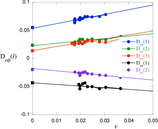
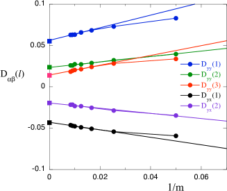
(a) (b)

Figure 1: Pair correlation function $D_{yy}(\ell)$ and $D_{yx}(\ell)$ for $4\times 3$, $U=4$ and $N_{e}=10$ obtained by the diagonalization quantum Monte Carlo method (a) and the Metropolis quantum Monte Carlo method (b). The square are the exact results obtained by the exact diagonalization method. In (a) the data fit using a straight line using the least-square method as the variance is reduced. We started with $N_{states}=100$ (first solid circles) and then increase up to 2000.

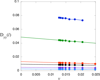
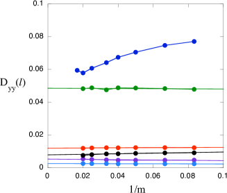
(a) (b)

Figure 2: Pair correlation function $D_{yy}(\ell)$ as a function of the energy variance $v$ in (a) and $1/m$ in (b) for $30\times 2$, $U=4$ and $N_{e}=48$. We used (a) the diagonalization quantum Monte Carlo method and (b) the Metropolis quantum Monte Carlo method. We set the open boundary condition. From the top, $\ell=(1,0)$, (2,0),(5,0), (4,0), (3,0) and (6,0).

3 Pair correlation functions

In this section, we present the results obtained by the QMC and QMD methods.

3.1 Comparison of two methods

The pair correlation function $D_{\alpha\beta}$ is defined by

$$D_{\alpha\beta}(\ell)=\langle\Delta_{\alpha}^{{\dagger}}(i+\ell)\Delta_{\beta}(i)\rangle,$$ (29)

where $\Delta_{\alpha}(i)$, $\alpha=x,y$, denote the annihilation operators of the singlet electron pairs for the nearest-neighbor sites:

$$\Delta_{\alpha}(i)=c_{i\downarrow}c_{i+\hat{\alpha}\uparrow}-c_{i\uparrow}c_{i+\hat{\alpha}\downarrow}.$$ (30)

Here $\hat{\alpha}$ is a unit vector in the $\alpha(=x,y)$-direction. We consider the correlation function of d-wave pairing:

$$P_{d}(\ell)=\langle\Delta_{d}(i+\ell)^{{\dagger}}\Delta_{d}(i)\rangle,$$ (31)

where

$$\Delta_{d}(i)=\Delta_{x}(i)+\Delta_{-x}(i)-\Delta_{y}(i)-\Delta_{-y}(i).$$ (32)

$i$ and $i+\ell$ denote sites on the lattice.

We show how the pair correlation function is evaluated in quantum Monte Carlo methods. We show the pair correlation functions $D_{yy}$ and $D_{yx}$ on the lattice $4\times 3$ in Fig.1. The boundary condition is open in the 4-site direction and is periodic in the other direction. An extrapolation is performed as a function of $1/m$ in the QMC method with Metropolis algorithm and as a function of the energy variance $v$ in the QMD method with diagonalization. We keep $\Delta\tau$ a small constant $\simeq 0.02\sim 0.05$ and and increase $\tau=\Delta\tau\cdot m$, where $m$ is the division number $m$ of the wave function $\psi$ in eq.(5). In the Metropolis QMC method, we calculated averages over $5\times 10^{5}$ Monte Carlo steps. The exact values were obtained by using the exact diagonalization method. Two methods give consistent results as shown in figures. All the $D_{yy}(\ell)$ and $D_{yx}(\ell)$ are suppressed on $4\times 3$ as $U$ is increased. In general, the pair correlation functions are suppressed in small systems.

In Fig.2, we show the inter-chain pair correlation function $D_{yy}(\ell)$ as a function of $1/m$ (b) and the energy variance (a) for the ladder model $30\times 2$. We use the open boundary condition. The boundary condition is not important for our purpose to check the consistency between QMC and QMD mthods. The number of electrons is $N_{e}=48$, and the strength of the Coulomb interaction is $U=4$. $\Delta_{y}(i)$ indicates the electron pair along the rung, and $D_{yy}(\ell)$ is the expectation value of the parallel movement of the pair along the ladder. The results obtained by two methods are in good agreement except $\ell=(1,0)$ (nearest-neighbor correlation).

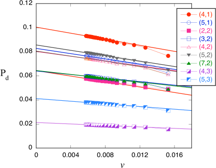
Figure 3: Pair correlation function $P_{d}$ as a function of the energy variance $v$ on $8\times 8$ lattice. $U=3$, $t^{\prime}=-0.2$ and the electron number is $N_{e}=54$. We have shown $P_{d}(\ell)=\langle\Delta_{d}(i+\ell)^{{\dagger}}\Delta(i)\rangle$ for $\ell=(m,n)-i$ and $i=(1,1)$, where $(m,n)$ are shown in the figure.

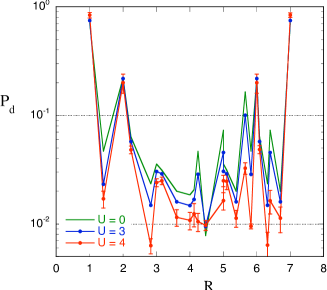
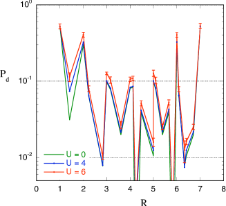
(a) (b)

Figure 4: Pair correlation function $P_{d}$ as a function of the distance $R=|\ell|$ on $8\times 8$ lattice for (a) the half-filled case $N_{e}=64$ and (b) $N_{e}=54$. We set $t^{\prime}=0.0$ and $U=0$, 3 and 4 for (a) and $t^{\prime}=-0.2$ and $U=0$, 4 and 6 for (b). To lift the degeneracy of electron configurations at the Fermi energy in the half-filled case, we included a small staggered magnetization $\sim 10^{-4}$ in the initial wave function $\psi_{0}$.

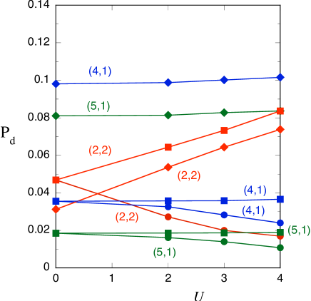
Figure 5: Pair correlation function $P_{d}$ as a function of $U$ on $8\times 8$ lattice. $t^{\prime}=-0.2$ for $N_{e}=54$ (diamonds), and $t^{\prime}=0$ for $N_{e}=50$ (squares) and $N_{e}=64$ (circles). We have shown $P_{d}(\ell)=\langle\Delta_{d}(i+\ell)^{{\dagger}}\Delta(i)\rangle$ for $\ell=(m,n)-i$ and $i=(1,1)$, where $(m,n)$ are shown in the figure.

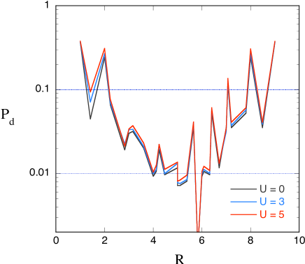
Figure 6: Pair correlation function $P_{d}$ as a function of the distance $R=|\ell|$ on $10\times 10$ lattice for $N_{e}=82$ and $t^{\prime}=-0.2$. The strength of the Coulomb interaction is $U=0$, 3 and 5.

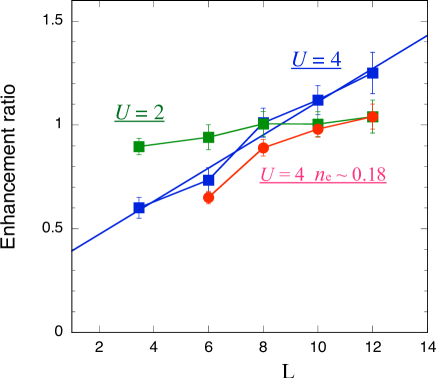
Figure 7: Enhancement ratio of pair correlation function $P_{d}|_{U}/P_{d}|_{U=0}$ as a function of the linear system size $L$ for $U=4$ and $U=2$. The electron density $n_{e}$ is about 0.8: $n_{e}\sim 0.8$ for squares. The data for $U=4$ and $n_{e}\sim 0.18$ are also shown by circles.

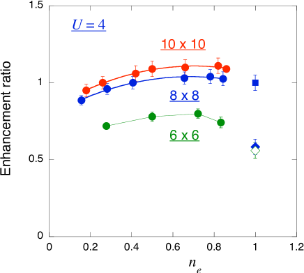
Figure 8: Enhancement ratio of pair correlation function $P_{d}|_{U}/P_{d}|_{U=0}$ as a function of the electron density $n_{e}$. We adopt $t^{\prime}=-0.2$ and $U=4$. For the half-filled case, the diamonds show that for $t^{\prime}=0$ on $8\times 8$ lattice (solid diamond) and $6\times 6$ lattice (open diamond). The square is for $t^{\prime}=-0.2$ on $8\times 8$ and $10\times 10$ where there is no enhancement.

3.2 Pair correlation in 2D Hubbard model

We present the results for pair correlation in the two-dimensional Hubbard model. In this section we show the results using the diagonalization QMC method because the Metropolis QMC method has a negative sign problem. We first examine the $8\times 8$ lattice. The $P_{d}$ was estimated by an extrapolation as a function of the variance $v$, as shown in Fig.3, where the computations were carried out on $8\times 8$ lattice with $U=3$, $t^{\prime}=-0.2$ and $N_{e}=54$. The extrapolation was successfully performed for $8\times 8$.

We consider the half-filled case with $t^{\prime}=0$; in this case the antiferromagnetic correlation is dominant over the superconductive pairing correlation and thus the pairing correlation function is suppressed as the Coulomb repulsion $U$ is increased. The Fig.4(a) exhibits the d-wave pairing correlation function $P_{d}$ on $8\times 8$ lattice as a function of the distance. The $P_{d}$ is suppressed due to the on-site Coulomb interaction, as expected. Its reduction is, however, not so considerably large compared to previous QMC studies [18] where the pairing correlation is almost annihilated for $U=4$. We then turn to the case of less than half-filling. We show the results on $8\times 8$ with electron number $N_{e}=54$. We show $P_{d}$ as a function of the distance in Fig.4(b) ($N_{e}=54$). In the scale of this figure, $P_{d}$ for $U>0$ is almost the same as that of the non-interacting case, and is enhanced slightly for large $U$. Our results indicate that the pairing correlation is not suppressed and is indeed enhanced by the Coulomb interaction $U$, and its enhancement is very small. The Fig.5 represents $P_{d}$ as a function of $U$ for $N_{e}=54$, 50 and 64. We set $t^{\prime}=0$ for $N_{e}=50$ and $t^{\prime}=-0.2$ for $N_{e}=54$ so that we have the closed shell structure in the initial function. In the system of this size, the effect of the inclusion of $t^{\prime}\neq 0$ is small. The Fig.6 shows $P_{d}$ on $10\times 10$ lattice. This also indicates that the pairing correlation function is enhanced for $U>0$. There is a tendency that $P_{d}$ is easily suppressed as the system size becomes small. We estimated the enhancement ratio compared to the non-interacting case $P_{d}(\ell)|_{U}/P_{d}(\ell)|_{U=0}$ at $|\ell|\sim L/2$ for $n_{e}\sim 0.8$ as shown in Fig.7. This ratio increases as the system size is increased. To compute the enhancement, we picked the sites, for example on $8\times 8$ lattice, $\ell=(3,2)$, (4,0), (4,1), (3,3), (4,2), (4,3), (5,0), (5,1) with $|\ell|\sim 4-5$ and evaluate the mean value. In our computations, the ratio increases almost linearly indicating a possibility of superconductivity. This indicates $P_{d}(\ell)\sim LP_{d}(\ell)\sim\ell P_{d}(\ell)$ for $\ell\sim L$. Because $P_{d}(\ell)|_{U=0}\sim 1/|\ell|^{3}$, we obtain $P_{d}(\ell)\sim\ell P_{d}(\ell)\sim 1/|\ell|^{2}$ for $|\ell|\sim L$. This indicatesthat the exponent of the power law is 2. When $U=2$, the enhancement is small and is almost independent of $L$. In the low density case, the enhancement is also suppressed being equal to 1. In Fig.8, the enhancement ratio is shown as a function of the electron density $n_{e}$ for $U=4$. A dome structure emerges even in small systems. The square in Fig.8 indicates the result for the half-filled case with $t^{\prime}=-0.2$ on $8\times 8$ lattice. This is the open shell case and causes a difficulty in computations as a result of the degeneracy due to partially occupied electrons. The inclusion of $t^{\prime}<0$ enhances $P_{d}$ compared to the case with $t^{\prime}=0$ on $8\times 8$ lattice. $P_{d}$ is, however, not enhanced over the non-interacting case at half-filling. This also holds for $10\times 10$ lattice where the enhancement ratio $\sim 1$. This indicates the absence of superconductivity at half-filling.

4 Summary

The quest for the existence of superconducting transition in the two-dimensional Hubbard model remains unresolved. Pair correlation functions had been calculated by using QMC methods, and their results were negative for the existence of superconductivity in many works. The objective of this paper was to reexamine this question by elaborating a sampling method of quantum Monte Carlo method.

We have calculated the d-wave pair correlation function $P_{d}$ for the 2D Hubbard model by using the QMC method. In the half-filled case $P_{d}$ is suppressed for the repulsive $U>0$, and when doped away from half-filling $N_{e}<N$, $P_{d}$ is enhanced slightly for $U>0$. It is noteworthy that the correlation function $P_{d}$ is indeed enhanced and is increased as the system size increases in the 2D Hubbard model. The enhancement ratio increases almost linearly $\propto L$ as the system size is increased, which an indicative of the existence of superconductivity. Our criterion is that when the enhancement ratio as a function of the system size $L$ is proportional to a certain power of $L$, superconductivity will be developed. This ratio dependes on $U$ and is reduced as $U$ is decreased. The dependence on the band filling shows a dome structure as a function of the electron density. In the $10\times 10$ system, the ratio is greater than 1 in the range $0.3<n_{e}<0.9$. This does not immediately indicates the existence of superconductivity. The size dependence is important and is needed to obtain the doping range where superconductivity exists. Let us also mention on superconductivity at half-filling. Our results indicates the absence of superconductivity in the half-filling case because there is no enhancement of pair correlation functions.

We have compared two methods: diagonalization QMC and Metropolis QMC. For small systems, the results obtained by two methods are quite consistent. When the system size is large, $P_{d}(\ell)$ is inevitably suppressed and almost vanishes if we use the Metropolis QMC method. $P_{d}(\ell)$ decreases as the division number $m$ increases in this method. We wonder if this excessive suppression of $P_{d}(\ell)$ is true. In fact, the correlation function $D_{yy}$ for the ladder Hubbard model obtained by the Metropolis QMC also shows a similar behavior when the size is increased, in contrast to enhanced $D_{yy}$ indicated by the density-matrix renormalization (DMRG) method[45]. The results by the diagonalization QMC are consistent with those of DMRG[21]. There is a possibility that this has some relation with the negative sign.

We thank J. Kondo, K. Yamaji, I. Hase and S. Koikegami for helpful discussions. This work was supported by Grant-in-Aid for Scientific Research from the Ministry of Education, Culture, Sports, Science and Technology in Japan. This work was also supported by CREST program of Japan Science and Technology Agency (JST). A part of numerical calculations was performed at facilities of the Supercomputer Center of the Institute for Solid State Physics, the University of Tokyo.

References

- [1] E. Dagotto, Rev. Mod. Phys. 66, 763 (1994).
- [2] D. J. Scalapino, in High Temperature Superconductivity- the Los Alamos Symposium - 1989 Proceedings, edited by K. S. Bedell, D. Coffey, D. E. Deltzer, D. Pines, J. R. Schrieffer, (Addison-Wesley Publ. Comp., Redwood City, 1990) p.314.
- [3] P. W. Anderson, The Theory of Superconductivity in the High-Tc Cuprates (Princeton University Press, Princeton, 1997).
- [4] T. Moriya and K. Ueda, Adv. Phys. 49, 555 (2000).
- [5] J. Hubbard, Proc. Roy. Soc. London, Ser A 276, 238 (1963).
- [6] J. E. Hirsch, Phys. Rev. Lett. 51, 1900 (1983).
- [7] J. E. Hirsch, Phys. Rev. B31, 4403 (1985).
- [8] S. Sorella, E. Tosatti, S. Baroni, R. Car and M. Parrinell, Int. J. Mod. Phys. B2, 993 (1988).
- [9] S. R. White, D. J. Scalapino, R. L. Sugar, E. Y. Loh, J. E. Gubernatis, and R. T. Scalettar, Phys. Rev. B40, 506 (1989).
- [10] M. Imada and Y. Hatsugai, J. Phys. Soc. Jpn. 58, 3752 (1989).
- [11] S. Sorella, S. Baroni, R. Car and M. Parrinello, Europhys. Lett. 8, 663 (1989).
- [12] E. Y. Loh, J. E. Gubernatis, R. T. Scalettar, S. R. White, D. J. Scalapino, and R. L. Sugar, Phys. Rev. B41, 9301 (1990).
- [13] A. Moreo, D. J. Scalapino, and E. Dagotto, Phys. Rev. B56, 11442 (1991).
- [14] N. Furukawa and M. Imada, J. Phys. Soc. Jpn. 61, 3331 (1992).
- [15] A. Moreo, Phys. Rev. B45, 5059 (1992).
- [16] S. Fahy and D. R. Hamann, Phys. Rev. B43, 765 (1991).
- [17] S. Zhang, J. Carlson and J. E. Gubernatis, Phys. Rev. B55, 7464 (1997).
- [18] S. Zhang, J. Carlson and J. E. Gubernatis, Phys. Rev. Lett. 78, 4486 (1997).
- [19] T. Kashima and M. Imada, J. Phys. Soc. Jpn. 70, 2287 (2001).
- [20] T. Yanagisawa, S. Koike and K. Yamaji, J. Phys. Soc. Jpn. 67, 3867 (1998).
- [21] T. Yanagisawa, Phys. Rev. B75, 224503 (2007). (arXiv: 0707.1929)
- [22] H. Yokoyama and H. Shiba, J. Phys. Soc. Jpn. 56, 1490 (1987); ibid. 56, 3582 (1987).
- [23] C. Gros, R. Joynt, and T. M. Rice, Phys. Rev. B36, 381 (1987).
- [24] T. Nakanishi, K. Yamaji and T. Yanagisawa, J. Phys. Soc. Jpn. 66, 294 (1997).
- [25] K. Yamaji, T. Yanagisawa, T. Nakanishi and S. Koike, Physica C 304, 225 (1998); Physica B284, 415 (2000).
- [26] S. Koike, K. Yamaji, and T. Yanagisawa, J. Phys. Soc. Jpn. 68, 1657 (1999); ibid 69, 2199 (2000).
- [27] T. Yanagisawa, S. Koike and K. Yamaji, Phys. Rev. B 64, 184509 (2001).
- [28] T. Yanagisawa, S. Koike and K. Yamaji, J. Phys.: Condens. Matter 14, 21 (2002).
- [29] T. Yanagisawa, M. Miyazaki, S. Koikegami, S. Koike, and K. Yamaji, Phys. Rev. B67, 132408 (2003).
- [30] T. Yanagisawa, M. Miyazaki and K. Yamaji, J. Phys. Soc. Jpn. 78, 013706 (2009).
- [31] M. Miyazaki, K. Yamaji and T. Yanagisawa, J. Phys. Soc. Jpn. 73, 1643 (2004).
- [32] L. T. Tocchio, F. Becca and C. Gros, Phys. Rev. B83, 195138 (2011).
- [33] H. Yokoyama, M. Ogata, Y. Tanaka, K. Kobayashi and H. Tsuchiura, J. Phys. Soc. Jpn. 82, 014707 (2013).
- [34] T. Mizusaki, M. Honma and T. Otsuka, Phys. Rev. C53, 2786 (1986).
- [35] L. F. Feiner, J. H. Jefferson, R. Raimondi, Phys. Rev. B53, 8751 (1996).
- [36] T. A. Maier, M. Jarrell, T. C. Schulthess, P. R. C. Kent, and J. B. White, Phys. Rev. Lett. 95, 237001 (2005).
- [37] T. Yanagisawa, J. Phys. Soc. Jpn. 79, 063708 (2010).
- [38] D. J. Scalapino, E. Loh, and J. E. Hirsch, Phys. Rev. B34, 8190 (1986)
- [39] N. E. Bickers, D. J. Scalapino, and S. R. White, Phys. Rev. Lett. 62, 961 (1989).
- [40] R. Hlubina, Phys. Rev. B59, 9600 (1999).
- [41] J. Kondo, J. Phys. Soc. Jpn. 70, 808 (2001).
- [42] T. Yanagisawa, New J. Phys. 10, 023014 (2008).
- [43] R. Blankenbecler, D. J. Scalapino, and R. L. Sugar, Phys. Rev. D24, 2278 (1981).
- [44] S. Sorella, Phys. Rev. B 64, 024512 (2001).
- [45] R. M. Noack, N. Bulut, D. J. Scalapino and M. G. Zacher, Phys. Rev. B56, 7162 (1997).