Effects of Penetrative Convection on Solar Dynamo
Abstract
Spherical solar dynamo simulations are performed. Self-consistent, fully compressible magnetohydrodynamic system with a stably stratified layer below the convective envelope is numerically solved with a newly developed simulation code based on the Yin-Yang grid. The effects of penetrative convection are studied by comparing two models with and without the stable layer. The differential rotation profile in both models is reasonably solar-like with equatorial acceleration. When considering the penetrative convection, a tachocline-like shear layer is developed and maintained beneath the convection zone without assuming any forcing. While turbulent magnetic field becomes predominant in the region where the convective motion is vigorous, mean-field component is preferentially organized in the region where the convective motion is less vigorous. Especially in the stable layer, the strong large-scale field with a dipole symmetry is spontaneously built up. The polarity reversal of the mean-field component takes place globally and synchronously throughout the system regardless the presence of the stable layer. Our results suggest that the stably stratified layer is a key component for organizing the large-scale strong magnetic field, but is not essential for the polarity reversal.
Subject headings:
convection–magnetohydrodynamics (MHD) – Sun: dynamo – Sun: interior1. Introduction
A grand challenge in the solar physics is a construction of self-consistent theory that explains the observed large-scale spatial structures of the fields and their dynamical change in time. Two basic large-scale structures that are left to be explained are the azimuthal average of the azimuthal flow, , and the azimuthal average of the azimuthal magnetic field, . The averaged velocity is characterized by the conical iso-rotation profile in the meridian plane and the thin tachocline layer with steep angular velocity gradient (e.g., Thompson et al. 2003). The averaged magnetic field is characterized by antisymmetric profile with respect to the equator and the polarity reversals with the pseudo-periodicity of years (e.g., Hathaway 2010). See Ossendrijver (2003) and Miesch (2005, 2012) for reviews.
To reproduce the large-scale structures and dynamics, magnetohydrodynamics (MHD) simulations have been performed both in the global (spherical shell) geometry (e.g., Gilman & Miller 1981; Gilman 1983; Glatzmaier 1985) and in the local Cartesian geometry (e.g., Meneguzzi & Pouquet 1989; Cattaneo et al. 1991; Nordlund et al. 1992; Brandenburg et al. 1996).
The first modern solar dynamo simulation with solar values of luminosity, background stratification, and rotation rate was performed by Brun et al. (2004). They solved anelastic MHD convection system in the domain that extends over –, spanning the bulk of the convection zone. While the solar-like equatorial acceleration and the dynamo-generated magnetic field with strengths of order G was achieved, the mean large-scale magnetic field were relatively weak and did not exhibit periodic polarity reversals.
Browning et al. (2006) showed, in anelastic spherical shell dynamo simulation with the presence of the tachocline, that strong axisymmetric toroidal magnetic fields can be formed in stably stratified layer below the convection zone. The associated mean poloidal magnetic fields showed the dipole dominance, but they did not exhibit polarity reversals. While the solar-like rotation profile was achieved in their simulations, a mechanical forcing was necessary to maintain the thin tachocline layer with steep angular velocity gradient.
Solar dynamo simulations that successfully produced the cyclic large-scale magnetic fields were presented in Ghizaru et al. (2010) and Racine et al. (2011). Their simulations are based on an anelastic model that is commonly used in the global circulation models of the earth’s atmosphere with a cooling term to force the system toward the ambient state (e.g., Prusa et al. 2008; Smolarkiewicz & Szmelter 2009). The solar-like thin tachocline layer was developed as a consequence of the cooling as well as the low dissipation embodied in their numerical scheme. They showed that the large-scale magnetic field is built up in the tachocline layer and exhibits polarity reversals when the temporal integration of the simulation was calculated for long enough.
The large-scale dynamo activity was found not only in the anelasic models but also in the compressible dynamo simulation. Käpylä et al. (2010) performed the dynamo simulation with the penetrative convection in a spherical-wedge geometry (e.g., Brandenburg et al. 2007). Using a weakly stratified dynamo model, they succeeded to simulate the formation and the cyclic polarity reversal of the large-scale magnetic field. Unlike Browning et al. (2006) and Ghizaru et al. (2010), the large-scale dynamo operated in the convection zone in their model. Despite the presence of the underlying stable layer below the convective envelope, the spontaneous formation of the solar-like tachocline layer was not observed.
These numerical studies that targeted for the solar dynamo have made it increasingly clear that the underlying stable layer below the convection zone is an important building block for the solar dynamo. It seems to play a crucial role in the formation of the solar-like & . However, there is no research that directly compares two dynamo simulations differing only in the presence and absence of the underlying stable layer.
In Miesch et al. (2009), the influence of the tachocline on the magnetic dynamo was reviewed by comparing two previous simulations done by Brun et al. (2004) and Browning et al. (2006). While two simulation models are both based on the same simulation code with solar values of the luminosity, rotation rate, and background stratification, they adopt different diffusivities and grid spacings that can affect the convective motion and magnetic dynamo. To get a better grasp of the role of the stably stratified layer in the solar dynamo mechanism, the influences of other parameters than the presence of the stable layer should be eliminated. This is one of motivations of our study.
In this paper, we perform fully compressible spherical solar dynamo simulation with a stably stratified layer below the convection zone. Formations of the key profiles of the solar interior, i.e., the solar-like & , and the spontaneous polarity reversals are reproduced without assuming any forcing in the fundamental equations. To elucidate the effects of the penetrative convection, two simulations with and without the stable layer below the convection zone are compared.
Another purpose of this paper is to report a development of new program code for the solar dynamo simulation. A lot of simulation models for the global dynamo are spectral-based type, using the spherical harmonics expansion (e.g., Brun et al. 2004). The spherical harmonics expansion method is, however, believed to be confronted with the parallel scaling difficulty when tens of thousands, or more, processor cores are used. A different approach to massively parallel solar dynamo model is strongly required for the present peta- or coming exa-scale era. We have developed a global solar dynamo simulation code based on the grid point-based approach.
The spherical geometry imposes difficulties in the design of the spatial grid points to sustain high numerical efficiency, accuracy, and parallel scalability. We have proposed an overset grid method approach to the spherical geometry (Kageyama & Sato 2004). The grid system, Yin-Yang grid, is applied to geodynamo (e.g., Kageyama et al. 2008; Miyagoshi et al. 2010), mantle convection (e.g., Kameyama et al. 2008; Tackley 2008), supernova explosions (e.g., Müller et al. 2012; Lentz et al. 2012), and other astro- and geophysical simulations. The parallel scaling property of the spherical MHD simulation on the Yin-Yang grid is promising. It attained % ( TFlops) of the peak performance of cores of the Earth Simulator supercomputer for the geodynamo simulations (Gordon Bell Award in Supercomputing 2004). Our new solar dynamo code is developed based on this Yin-Yang geodynamo code. This paper is our first report on the results obtained by this Yin-Yang solar dynamo code.
2. Numerical Settings

We numerically solve an MHD dynamo convection system in a spherical shell domain defined by , , and , where , and are radius, colatitude, and longitude, respectively. Our model has two layers: upper convective layer of thickness in the range of , and stably stratified lower layer of thickness in .
The fundamental equations are the fully compressible MHD equations in the rotating frame of reference with a constant angular velocity which is parallel to the coordinate axis ():
| (1) | |||||
| (2) | |||||
| (3) | |||||
| (4) |
with
Here the mass density , pressure , mass flux , magnetic field’s vector potential are the basic variables. We assume an ideal gas law with , where is the internal energy. The viscosity, electrical resistivity, and thermal conductivity are represented by , , and respectively.
The initial condition is a hydrostatic equilibrium which is described by a piecewise polytropic distribution with the polytropic index ,
| (5) |
(e.g., Käpylä et al. 2010). We choose and for the upper convection layer and the lower stable layer, respectively. The thermal conductivity is determined by requiring a constant luminosity , defined by , throughout the domain.
We solve the MHD equations in a non-dimensional form. Normalization quantities are defined by setting where is the initial density at . We normalize length, time, velocity, density, and magnetic field in units of , , , and . We define the Prandtl, magnetic Prandtl, and Rayleigh numbers by
| (6) |
where is the density at the mid-convection zone (), and is the depth of the convection zone. The stratification level is controlled by the normalized pressure scale height at the surface,
| (7) |
where is the temperature at . In this work, we use , yielding a small density contrast about . Figure 1 shows the radial distributions of the initial temperature, density and pressure adopted for our numerical model by solid, dashed and dash-dotted curves, respectively. The vertical axis is normalized by the value at . The radial slopes in our numerical model are more gentle than the solar profiles. These give the convective motion with the Mach number of .
The relative importance of rotation in the convection is measured by the Coriolis number
| (8) |
where is the mean velocity. The double angular brackets denote the time and volume average in the convection zone in the saturated state. The convective turn-over time and the equipartition strength of magnetic field are defined, respectively, by
| (9) |
The stress-free boundary condition for the velocity is imposed on the two spherical boundaries. We assume the perfect conductor boundary condition for the magnetic field () on the inner surface, and the radial field condition () on the outer surface. A constant energy flux is imposed on the inner boundary. The temperature is fixed to be on the outer boundary.
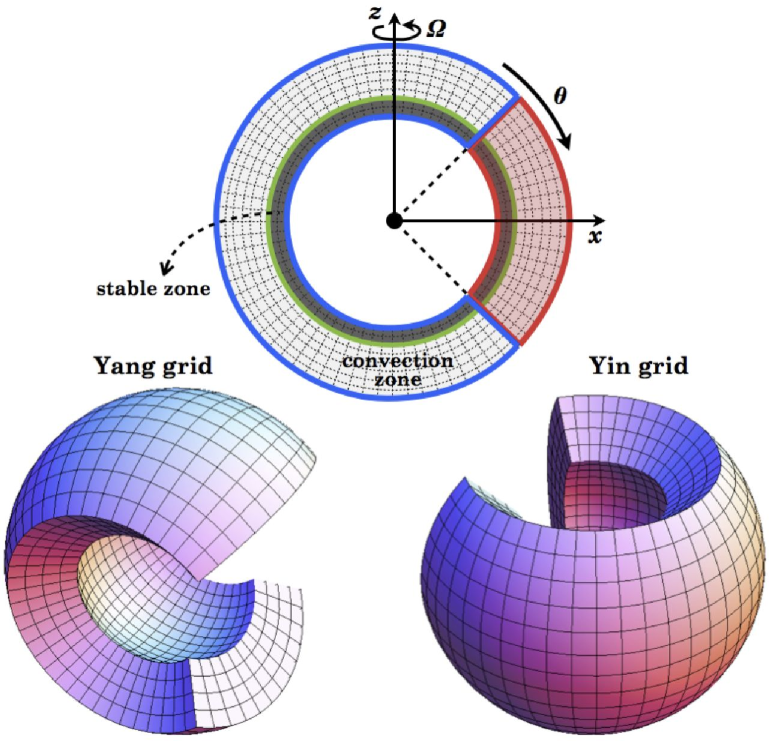
The eqs. (1)–(4) are discretized by the second-order central difference on the Yin-Yang grid. Each of the two congruent grids, Yin-grid and Yang-grid, covers a partial spherical shell region defined as (). They are combined in a complemental way to cover a whole spherical shell as shown in Figure 2. The regions surrounded by red and blue curves are assigned to the Yin- and Yang-grids, respectively. Physical quantities on the horizontal boarders of Yin- or Yang-grid are set by mutual interpolations. For the time integration, the standard fourth-order Runge-Kutta method is used. Since the Yin-Yang grid is free from the coordinate singularity and the grid concentration around there, we can avoid the severe time-step constraint due to the CFL condition. See Kageyama & Sato 2004 for details on the Yin-Yang grid method. The computation is performed in parallel using MPI (Message Passing Interface).
Non-dimensional parameters , , and , and constant angular velocity of are adopted in all the calculations reported here in order to achieve the Coriolis number expected in the convection zone of the Sun []. The total grid size for the run with the upper convection layer and the lower stable layer (Model A) is (in ) (in ) 402 (in ) (Yin & Yang). A model without the stable layer (Model B) is also studied, in the domain , with the same physical parameters and the same grid spacings (). A random temperature perturbation and weak magnetic field are seeded in the convection zone when the calculation starts.
3. Numerical Results
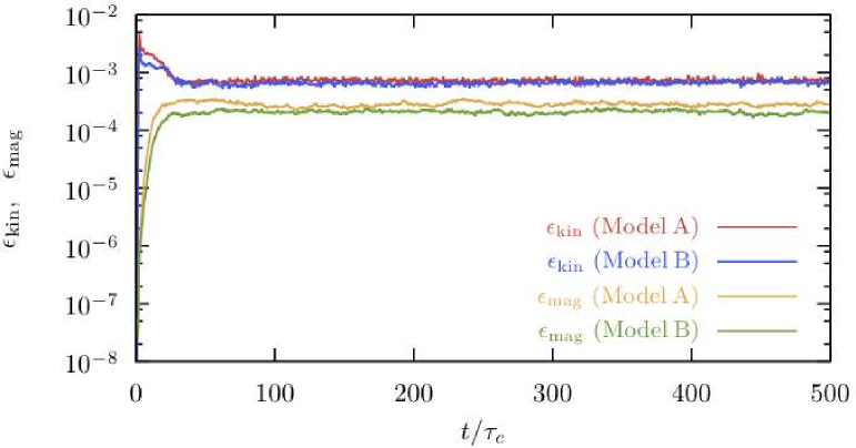
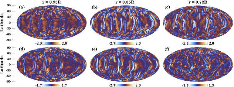
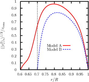
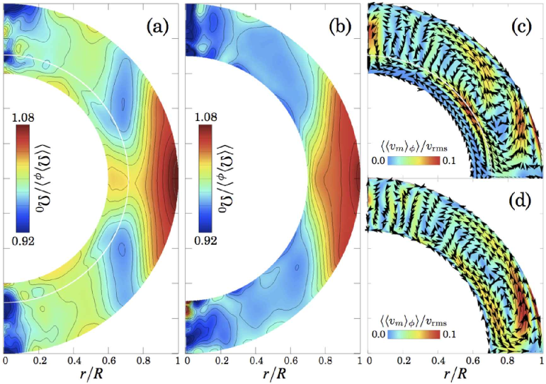
Figure 3 shows the temporal evolution of the volume-averaged kinetic and magnetic energies defined by
| (10) |
for Models A and B. The red and orange curves correspond to those for Model A. The blue and green curves are for Model B. After the convective motion sets in, it reaches a nonlinear saturation state at around . The saturation levels of the convection kinetic energy for Models A and B are almost the same. The mean velocity is which yields , and for both models. We have run the simulations till and then compare physical properties of convections, mean flows and magnetic dynamos between two models.
To examine the convective and magnetic structures in detail, we define the following four averages of a function on a sphere.
The latitudinal average:
| (11) |
The longitudinal average:
| (12) |
The spherical average:
| (13) |
The northern hemispheric average:
| (14) |
The time-average of each spatial mean is denoted by additional angular brackets, such as .
3.1. Properties of Convective Motion
Figure 4 shows, in the Mollweide projection, the distribution of the radial velocity when on spherical surfaces at different depths for two models. Panels (a)–(c) correspond to the depths , and for Model A, and panels (d)–(f) are those for Model B. The orange and blue tones depict upflow and downflow velocities. At the upper () and mid () convection zones, the convective motion is characterized by upflow dominant cells surrounded by networks of narrow downflow lanes for both models. The higher the latitude, the smaller the convective cell prevails. Elongated columnar convective cells aligned with the rotation axis appear near the equator. These are the typical features observed in rotating stratified convection (e.g., Spruit et al. 1990; Miesch et al. 2000; Brummell et al. 2002; Brun et al. 2004). In panel (c), we find that the downflow lanes persist the plume-like coherent structure even just above the bottom of the unstable layer (). The downflow plumes then penetrate into the underlying stable layer.
The radial profile of the mean radial velocity is shown in Figure 5. The red-solid and blue-dashed curves correspond to Models A and B, respectively. The time average spans in the range of . The mean radial velocity has a peak at the mid convection zone () for both models. The convective motion is the most active there. While the radial flow is restrained by the boundary placed on the bottom of the convection zone in Model B, it can penetrate into the underlying stable layer in Model A. As a result of the penetrative convection, mean zonal and meridional flows are driven by the Reynolds and Maxwell stresses in the stable layer. That will be described in the followings.
3.2. Structures of Mean Flow
In Figures 6(a) and (b), time-averaged mean angular velocity, defined by , is shown for the models A and B, respectively. The time average spans in the range of . The normalization unit is the initial angular velocity .
The differential rotations in both models have basically solar-like profiles with the equatorial acceleration. However, both exhibit more cylindrical alignment than the solar rotation profile characterized by the conical iso-rotation surface. The system is dominated by the Taylor-Proudman balance in both models (e.g., Pedlosky 1987). The angular velocity contrast between equator and pole is about % in Model A and % in Model B. These are slightly smaller than that obtained by the helioseismology (%). More remarkably, a radial gradient of the angular velocity is developed in the stably stratified layer around latitudes . This structure is reminiscent of the solar tachocline despite the radial shear layer is broad compared to the observed one (Spiegel & Zahn 1992; Charbonneau et al. 1999; Miesch 2005; Hughes et al. 2007). The rotation profile of Model A is reasonably similar with that of the Sun deduced from helioseismology (Thompson et al. 2003).
The spontaneous formation of the tachocline-like shear layer below the convective envelope was reported in the hydrodynamic simulation of the solar penetrative convection performed by Brun et al. (2011). Our results suggest that the tachocline-like shear layer is a natural outcome of the presence of the stable layer even in the MHD convection system. We discuss more about the differential rotation profile established in Model A in § 4.1.
Shown in Figures 6(c) and (d) are time-averaged mean meridional flows for the models A and B. The color contour depicts the meridional flow velocity, defined by , with a maximum . Overplotted are streaklines with a length proportional to the flow speed. The circulation flow is primarily counter-clockwise in the bulk of the convection zone in the northern hemisphere, that is, the poleward in the upper convection zone and the equatorward in the bottom convection zone in both models. There is however a clear difference in the circulation pattern between the two models. While a large single-cell is formed in Model B, Model A shows a double-cell pattern with a strong inward/outward flow at the low/mid latitudes. An intriguing finding is that the equatorward component penetrates into the underlying stable layer when the radial gradient of the angular velocity resides (see Figure 6(a)). This suggests that the penetrative transport of magnetic flux by the meridional flow might play a role in magnetic dynamo in our model.
The meridional flow takes a role in transporting angular momentum and magnetic flux in the Sun. However, the circulation pattern, velocity, and their time variations are still controversial as compared with the mean angular velocity profile which is well-confirmed by the helioseismic measurement. This is because the meridional circulation is much weaker than the differential rotation. Although the global circulation consisting of two cells is implied by the helioseismic inversion (see Mitra-Kraev & Thompson 2007) and is also obtained by numerical simulation (e.g., Miesch et al. 2006), it is not agreed in general (Hathaway 2012; Schad et al. 2012).
The mean-field theory of the angular momentum transport predicts a single-cell circulation (c.g., Ruediger 1989). Despite the kinematic flux-transport dynamo model is constructed based on the single-cell circulation (Dikpati & Charbonneau 1999; Charbonneau 2005), the influence of the circulation pattern on the magnetic activity is still a matter of debate (Pipin & Kosovichev 2013 and references therein). In order for more detailed discussion about the meridional flow, we should improve our simulation model in such a way to achieve smaller-scale subsurface convection ranging from granulation to super-granulation as probed by local helioseismology (Gizon & Birch 2005; Rieutord & Rincon 2010).
3.3. Structures of Magnetic Field
.
|
|
|
|
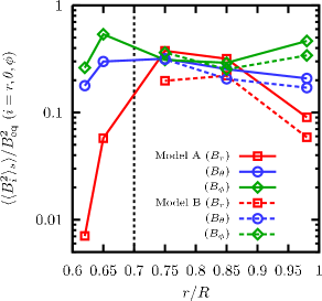
As shown in Figure 3, the magnetic energy is amplified by the dynamo action and is saturated at a level of about % of the convective kinetic energy for both models after . The magnetic field is maintained longer enough than the magnetic diffusion time (). Although the volume-averaged magnetic energy is almost the same in the models A and B, there are remarkable differences in the spatial structure of the magnetic fields.
The time and surface average of the magnetic energy density is presented as a function of radius in Figure 7. The broken solid lines with red-squares, blue-circles and green-diamonds denote the contributions from radial, latitudinal and azimuthal components of the magnetic field for Model A. The broken dashed lines with the same symbols denote those for Model B. The time average spans in the range of . While the contributions of three magnetic components are almost the same at the mid convection zone () where the convective motion is vigorous, the azimuthal component becomes predominant in the region where the convective motion is less active for both models (see also Figure 5). Especially, in the stable layer of Model A, most of the magnetic energy is stored as a form of the azimuthal field.
To examine the magnetic structure in more detail, we divide the magnetic energy density into axi-symmetric part and asymmetric part (see Appendix)
| (15) |
where we denote the axi-symmetric part of the magnetic field for ,
| (16) |
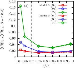
To elucidate the relative strengths of axi-symmetric components, we plot the profiles of in Figure 8(a). The broken solid lines with red-squares, blue-circles and green-diamonds denote the radial, latitudinal and azimuthal components for Model A. The broken dashed lines with the same symbols denote those for Model B. The time average spans in the range of . Among the three axi-symmetric components, is dominant. The tendency of –dominance is apparent not only in the stable layer, but also in the convection zone both in models A and B. The relative strength of the axi-symmetric component increases with the depth and reaches the maximum at around the bottom stable zone. Figures 7 and 8(a) suggest that the axi-symmetric component is built up rather in the convectively calm layer although the magnetic energy is amplified preferentially in the region where the vigorous convective motion exits.
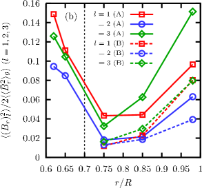
We then analyze the latitudinal moments of the axi-symmetric field . We focus on since this component reflects purely the poloidal field, while and are mixture of the toroidal and poloidal fields. From the Peseval’s equation (see Appendix),
| (17) |
where
| (18) |
Here are normalized Legendre polynomials. Figure 8(b) shows profiles of for and . The broken solid lines with red-squares, blue-circles and green-diamonds denote dipole (), quadrupole (), and octupole () moments for Model A. The broken dashed lines with the same symbols denote those for Model B. The time average spans in the range of . There is not much difference among amplitudes of dipole, quadrupole and octupole moments at all the depth. Nevertheless, it would be worth noting that Model B has a octupole dominance in almost the whole domain. In the case of Model A, the dipole gradually becomes dominant with the depth. It is predominant in the bottom convection zone and the stable zone although the upper and mid convection zones are dominated by higher multipoles like as Model B. The stably stratified layer below the convective envelope promotes dipole solution as indicated by Miesch et al. (2009).
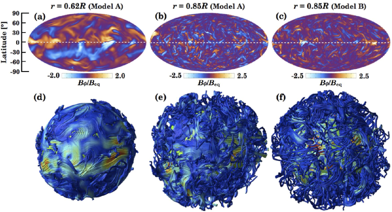
The similarity and difference of the magnetic structure between two models are the most obvious on the azimuthal component of the magnetic field. A snapshot of the azimuthal component of the magnetic field at is presented in Figure 9 on a spherical surface at (a) and (b) for Model A, and (c) for Model B. The orange and blue tones depict positive and negative values of the component normalized by . The magnetic field lines at the time corresponding to those in the panels (a)–(c) are visualized in Figures 9(d)–(f), respectively. As expected from Figures 7 and 8, the convective envelope is dominated by disordered tangled magnetic field lines with a myriad of localized small-scale structures in both models. These incoherent magnetic fields are strongly influenced by vigorous convective motions and thus are highly intermittent. The horizontal converging flows sweep magnetic fields into downflow lanes and intensify them locally to the super-equipartition strength as was observed in existing convective dynamo simulations (e.g., Brandenburg et al. 1996; Cattaneo et al. 2003; Brun et al. 2004).
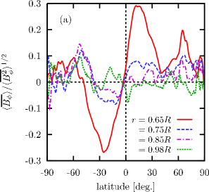
In the underlying stable layer of Model A, a strong large-scale azimuthal component of magnetic field is built up around the equator, and resides there for long time intervals. This well-organized magnetic component is roughly antisymmetric about the equatorial plane and has a maximum strength of an order of . The large-scale component is organized in the stable zone where the radial angular velocity gradient resides (see Figure 6(a)). This would be an important evidence of a connection between the deep-seated large-scale magnetic component and the tachocline-like shear layer that is spontaneously developed in the model with the stable layer.
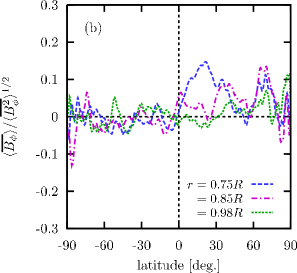
The latitudinal profiles of are shown at the sampled radii in Figures 10(a) and (b) for Models A and B. The red-solid, blue-dashed, purple-dash-dotted and green-dotted curves correspond to , , , and , respectively. The time average spans in the range of for Model A or for Model B. As shown in Figures 8(a) and 9, the strong mean azimuthal component with the antisymmetric profile is built up around the equatorial plane in the stable layer of Model A. It reaches maximum strength at around the latitude . While the antisymmetric property of the mean-field is found not only in the stable layer but also in the convective envelope, the amplitude of the mean-field component is much smaller in the convection zone than in the stable zone. In comparison with the Model A, the antisymmetric property of the mean azimuthal field is weaker in the Model B.
Overall magnetic structures simulated in our models indicate that the stably stratified layer is an important building block to organize large-scale magnetic components and support numerical studies of Browning et al. (2006) and Ghizaru et al. (2010). Despite the magnetic energy is amplified by the vigorous convective motion in the mid convection zone, the strong mean magnetic component is preferentially organized in the region where the convective motion is less vigorous. This suggests that the downward pumping process of the magnetic flux is of great importance in the solar dynamo mechanism (Tobias et al. 2001, 2008; Barker et al. 2012). The implementation of more realistic convective penetration and downward pumping processes into the numerical modeling might come the first to reproduce the solar dynamo.
3.4. Cyclic Property of Magnetic Fields
|
|
|
|
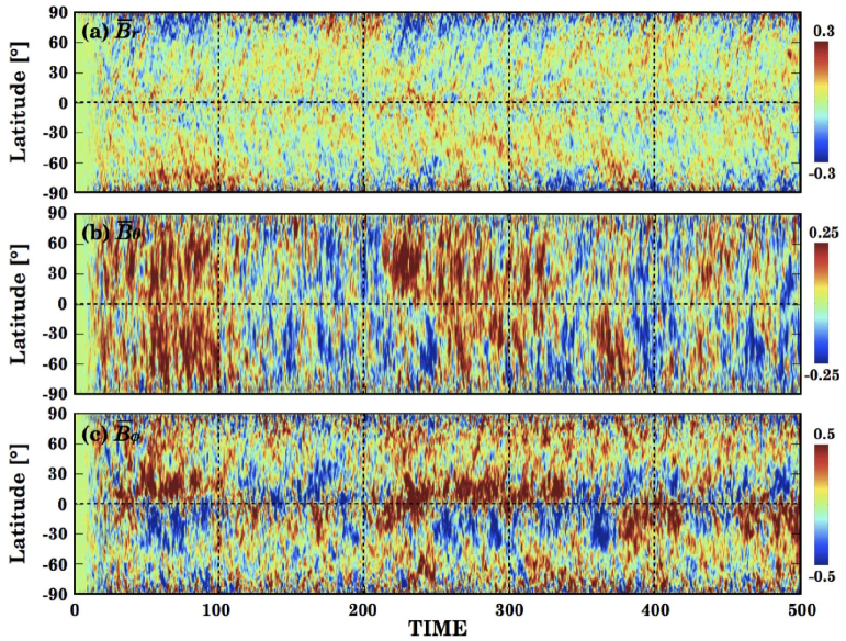
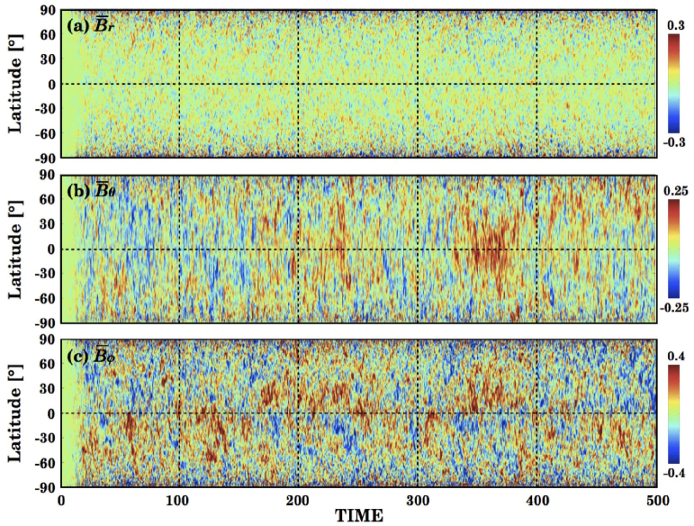
One of the most interesting findings in our simulation is that the large-scale magnetic fields show polarity reversals. Figure 11 gives an azimuthally-averaged magnetic field as a function of time and latitude for Model A. The panels (a), (b) and (c) represent , , and at . The large-scale with antisymmetric parity persists over a relatively long period despite strong stochastic disturbances due to penetrative convective motions. The component changes the sign for at least three times, at about , , and [panel (c)].
As for the poloidal component of the magnetic field, it shows the dipole dominance in the stable layer as indicated in Figure 8(b). During – when strong component with positive polarity dominates in the northern hemisphere, negative and positive are observed [panels (a) and (b)]. While the component has the same sign in both the hemispheres, the component has opposite polarity in the two hemispheres. When the reversal takes place, the other two components and also change the sign. See, for example, at about in Figure 11.
The time-latitude diagram of an azimuthally-averaged magnetic field for Model B is shown in Figure 12. The panels (a), (b) and (c) represent , , and at . The mean-field component shows a week polarity preference and polarity reversals in time even in the model without the stable layer. While the component has an antisymmetric profile with respect to the equator, the component has the same sign in both the hemispheres as well as the Model A. However, the amplitude, coherency and dipole dominance of the mean magnetic component are much weaker in the model B compared with those in the model A. These are consistent with Figures 8–10.
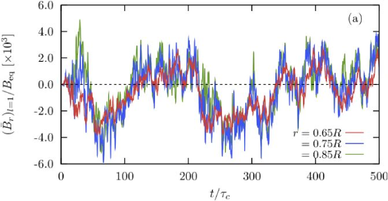
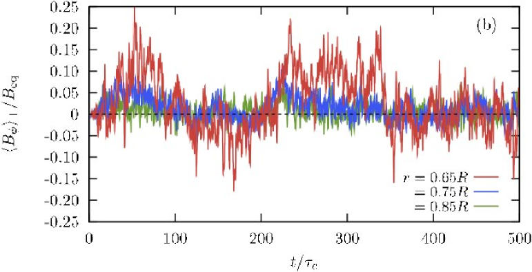
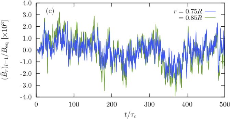
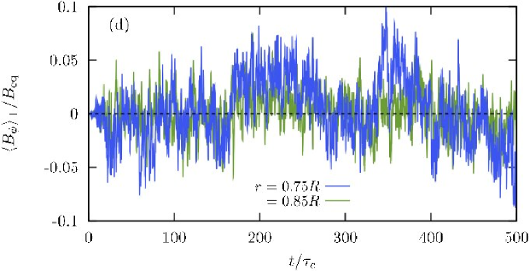
As the indicators of the depth-dependency of the polarity reversal, we show the temporal evolution of the dipole moment defined by equation (18) and the northern hemispheric average of the azimuthal field in Figure 13. Panels (a) and (b) correspond to and for Model A. Panels (c) and (d) are those for Model B. The red, blue, and green curves correspond to the depths , , and , respectively. The polarity reversal takes place not only in the underlying stable layer but also in the convective envelope for Model A. It is remarkable that there is a clear phase synchronization in the polarity reversals at different depths. Even in the case of the Mode B, the polarity reversal of the mean-field component is noticeable although the short-term variability is superimposed onto the global long-term modulation. The cycle period is about for both models. This indicates that the polarity reversal of the mean-field component is a global phenomenon that takes place synchronously throughout the system regardless the presence of the stable layer.
4. Discussion
4.1. Force Balance in Differential Rotation

|
|
|
|
The helioseismic measurements suggest that the tachocline thickness is less than % of the solar radius (e.g., Elliott & Gough 1999; Charbonneau et al. 1999; Basu & Antia 2001). The presence of such a thin transition layer leads to the tachocline confinement problem (Spiegel & Zahn 1992). The mechanism that inhibits the differential rotation in the convection zone to spread into the deeper radiative interior is still an open problem, though several theoretical models have been proposed (Rudiger & Kitchatinov 1997; Gough & McIntyre 1998; Rogers 2011; Brun et al. 2011).
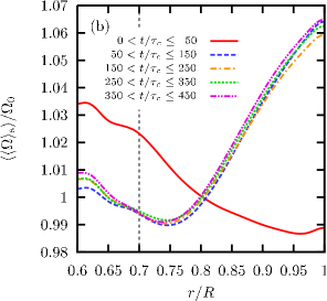
In conjunction with the tachocline confinement problem, we examine the time evolution of the differential rotation established in our simulation model with the stably stratified layer (Model A). We show, in Figure 14 (a), the temporal evolution of the kinetic energy of differential rotation averaged over the entire volume () and the volume of the stable zone ( ) defined by
| (19) |
After the initial transitional stage , the kinetic energy of the differential rotation is settled into an approximately constant value both in the entire domain and in the stable zone. In our simulation, the viscous spreading of the tachocline-like shear layer operates on a timescale of . This dominates over the radiative spreading controlled by the Eddington-Sweet timescale. Since the duration of the simulation is about , the differential rotation has achieved the equilibrated profile.
The statistical stationarity of the differential rotation profile is confirmed in Figure 14 (b), which shows the radial profile of the mean angular velocity averaged over a given time span, , for Model A. The different lines correspond to different time spans. Here the surface average is taken over the range of (around the equator). After the initial evolutionary stage (), the differential rotation attains a stationary profile in which outer shell is rotating faster. The differential rotation in the convection zone does not spread downward into the stable layer as time passes in spite of the shear on the interface of the convection and stable layers.
The formation of the solar-like rotation profile is associated with the development of the magnetic field. As seen in the mean rotation profile during , the inner shell rotates faster than the outer shell at the early dynamo kinematic stage. When the magnetic field is sufficiently amplified, it begins to affect the convective motion. The rotation profile changes to the opposite state in which the outer shell is rotating faster. This implies that the dynamo-generated magnetic field plays an important role in establishing the solar-like differential rotation.
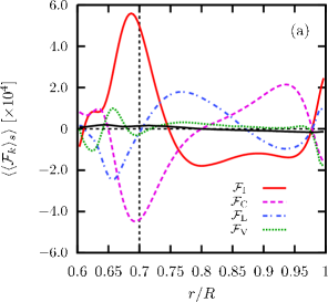
To elucidate the azimuthal force balance maintaining the differential rotation, we will consider the azimuthal component of momentum equation. The right-hand side of the equation is divided into four force terms:
| (20) |
where is the inertia force, is the Coriolis force, is the Lorentz force, and is the viscous force. Note that azimuthal pressure gradient force does not contribute to the mean azimuthal force balance. These four force terms should cancel out each other for retaining the statistical equilibrium.
The time and surface average of the each force term is demonstrated as a function of radius in Figure 15 (a). The solid red, dashed magenta, dash-dotted blue, dotted green curves correspond to the radial profiles of the inertia, Coriolis, Lorentz and viscous forces, respectively. The solid black curve denotes the sum of the four azimuthal forces. The time average is taken over with snapshot data. The azimuthal force balance is mainly dominated by the inertia, Coriolis and Lorentz forces. In the convection zone, the negative inertia force balances with the sum of the positive Coriolis and Lorentz forces. In contrast to that, the positive inertia force is compensated by the sum of the negative Coriolis and Lorentz forces in the stable zone. The positive peak of below the interface between the convection zone and stable zone indicates the angular momentum transport by the penetrative convection. The viscous force makes a minor contribution to the azimuthal force balance except the surface layer and the bottom of the stable zone. The net azimuthal force represented by solid black curve is nearly zero, confirming the statistical equilibrium of the azimuthal flow not only in the convection zone, but also in the stable zone.
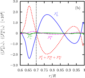
To examine the azimuthal force balance in more detail, we divide each force term into the contributions of the axisymmetric mean components given by and the contributions of the fluctuation components by . Figure 15 (b) illustrates the roles of the mean and fluctuation components in the azimuthal force balance. Here we show the radial profiles of and by the red dashed and magenta dashed curves, which are all flow origins. The blue and green solid curves denote the radial profiles of and , which are magnetic field origins. The contributions of fluctuation components to Coriolis and viscous forces are negligibly small.
In the region where the convective motion is less vigorous (upper convection zone and stable zone), the positive azimuthal force due to the flow field is balanced with the negative force sustained by the dynamo-generated magnetic field. In contrast to that, the negative azimuthal force due to the flow field is compensated by the positive Lorentz force in the most of the convection zone where the convective motion is vigorous. The Lorentz force by the nonlinear coupling of fluctuating magnetic field plays a crucial role in the azimuthal force balance for maintaining the equilibrated profile of the differential rotation.
As shown in Figure 6, the differential rotation profile established in our model exhibits more cylindrical alignment than the solar rotation profile characterized by the conical iso-rotation surface. Our MHD convection system is still dominated by Taylor-Proudmann balance. It is well known that the latitudinal entropy variation at the base of the convection zone induces a baroclinicity, and yields the solar-like conical rotation profile (e.g., Kitchatinov & Ruediger 1995; Rempel 2005; Miesch et al. 2006; Masada 2011). It might be important to numerically capture with higher accuracy the nonlinear MHD processes, such as instabilities and resultant turbulence, in the stable layer to reproduce the large-scale solar convection profile more accurately.
4.2. Qualitative Picture of Magnetic Dynamo
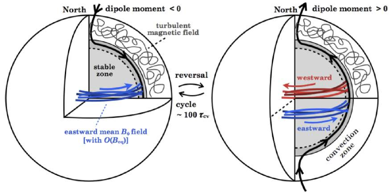
Since the main purpose of this paper is not to accurately model the solar dynamo, but rather to reveal the effects of the penetrative convection on the magnetic dynamo process, the effective luminosity used in the simulation are larger than the solar values. Nevertheless, it would be helpful to evaluate the cycle period and the mean-field strength obtained in our simulation in comparing our model with the models of other groups.
Figures 13 gives the cycle period of the polarity reversal , which is evaluated as
| (21) |
when we adopt the solar values and . This is about a half of the cycle of the polarity reversal in the Sun. At the cycle maxima, the strength of the axi-symmetric azimuthal field in the stable zone reaches , which can be evaluated as
| (22) |
with the density at the mid convection zone of the Sun. This is a comparable strength with the large-scale magnetic field simulated in Browning et al. (2006) and Ghizaru et al. (2010), but would be an order of magnitude smaller than that expected in the tachocline layer of the Sun for explaining the sunspot emergence at the surface on latitudes of less than (c.g., Choudhuri & Gilman 1987)
When taken all the numerical results together, the structure and evolution of the dynamo-generated magnetic field in our model is represented by a schematic picture in Figure 15. The thick black line demonstrates the poloidal magnetic component with dipole dominance. The blue and red curves denote eastward and westward azimuthal components. The mean large-scale azimuthal field with is preferentially organized around the equatorial region in the stably stratified layer, whereas the convection zone is dominated by the turbulent fluctuating component. The polarity reversal with the cycle period of takes place globally and synchronously throughout the system.
The dipole dominance is one of remarkable features of the large-scale magnetic field rooted in the stable layer. The tendency of the dipole dominance that appears when taking account of the stable layer is reported in Browning et al. (2006) and Miesch et al. (2009). The differential rotation can not only amplify the mean toroidal fields through the so-called -effect, and but also expel the asymmetric field components via rotational smoothing process (Rädler 1980, 1986; Spruit 1999). The dipole-like magnetic structure with large-scale axi-symmetric azimuthal component would be thus a natural outcome of the rotational amplification and smoothing of the magnetic field in the stable layer. The more accurate modeling of the stably stratified tachocline would enable us to tackle the generation mechanism of large-scale field that can be responsible for the origin of the sunspot on the solar surface.
We finally remark that both the equatorward migration and buoyant emergence of the large-scale magnetic component, that can bridge the gap between the simulation and sunspot observation, could not be simulated in our model. This clearly tells us that we have still a lot of missing ingredients to reproduce the solar interior in our dynamo modeling.
5. Summary
We reported, in this paper, our first results of solar dynamo simulation based on the Yin-Yang grid with the fully compressible MHD model. To investigate influences of the stably stratified layer below the convection zone, two simulation models with and without the stable layer (Models A and B) were compared. It is confirmed from our numerical study that the stable layer has substantial influence on the convection and the magnetic field. Our main findings are summarized as follows.
1. The convective motion in the upper convection zone is characterized by upflow dominant cells surrounded by networks of narrow downflow lanes for both models. While the radial flow is restrained by the boundary placed on the bottom of the convection zone in Model B, the downflow lanes persist the plume-like coherent structure even just above the bottom of the unstable layer in Model A. The downflow plumes then penetrate into the underlying stable layer.
2. The differential rotation profiles in both models are reasonably solar-like with equatorial acceleration. However, both exhibit more cylindrical alignment than the solar rotation profile with the conical iso-rotation surface inferred from the helioseismology. It is remarkable that the radial shear layer, which is reminiscent of the solar tachocline, is spontaneously developed without any forcing just beneath the convection zone as a result of the penetrative convection in Model A. The Lorentz force by the nonlinear coupling of fluctuating magnetic field plays an important role in the azimuthal force balance for maintaining the solar-like differential rotation.
3. While the turbulent magnetic field becomes predominant in the region where the convective motion is vigorous, the mean-field component is preferentially built up in the region where the convective motion is less vigorous. Especially in the stably stratified layer, the strong large-scale azimuthal component with antisymmetric profile with respect to the equator and the poloidal field with dipole dominance are spontaneously organized.
4. The mean magnetic component undergoes polarity reversals with the cycle period of for both models. It takes place globally and synchronously throughout the system regardless the presence of the stable layer. However, the amplitude, coherency and dipole dominance of the mean magnetic component are much weaker in the model B compared with those in the model A. The stably stratified layer is a key component for organizing the large-scale strong magnetic field, but is not essential for the polarity reversal.
All the dynamo simulations reported here have used a relatively weak stratification with the density contrast of about (see §2). The strong stratification in the actual Sun may influence on the physical properties of convections, mean flows and magnetic dynamo (Käpylä et al. 2013). It would be interesting that the three key features, solar-like , , and the polarity reversals are self-consistently reproduced, without assuming any forcing, even in the modest density stratification. Higher resolution simulations with a more realistic density stratification will facilitate our understanding of the physics of the solar convection and the solar dynamo, that is our next step with the Yin-Yang solar dynamo simulation code.
Appendix A Dividing spherical mean of energy into axi-symmetric and asymmetric parts
The purpose of this section is to split the spherical mean of energy into axi-symmetric part and asymmetric part.
For a smooth function on a sphere, we define the following three means.
Longitudinal mean:
| (A1) |
Latitudinal mean:
| (A2) |
Surface mean:
| (A3) |
We can always divide into axis-symmetric and asymmetric parts:
| (A4) |
Note that
| (A5) |
The surface mean of is also divided into two parts:
| (A6) | |||||
| (A7) | |||||
| (A8) |
Expanding by the normalized Legendre polynomials
| (A9) |
that satisfy
| (A10) |
as
| (A11) |
we get the Perseval’s equation,
| (A12) |
where Legendre coefficients are given by
| (A13) |
Similarly, for a vector field , we get
| (A14) | |||||
| (A15) | |||||
| (A16) |
where the symmetric part
| (A17) |
and asymmetric part
| (A18) |
Due to the Perseval’s equation (A12), each of the three terms in eq. (A17) can be expanded as,
| (A19) |
where are Legendre coefficients
| (A20) |
Note that for a magnetic field, the monopole component is absent.
References
- Basu & Antia (2001) Basu, S., & Antia, H. M. 2001, MNRAS, 324, 498
- Barker et al. (2012) Barker, A. J., Silvers, L. J., Proctor, M. R. E., & Weiss, N. O. 2012, MNRAS, 424, 115
- Brandenburg et al. (1996) Brandenburg, A., Jennings, R. L., Nordlund, Å., et al. 1996, Journal of Fluid Mechanics, 306, 325
- Brandenburg et al. (2007) Brandenburg, A., Käpylä, P. J., Mitra, D., Moss, D., & Tavakol, R. 2007, Astronomische Nachrichten, 328, 1118
- Brown et al. (2011) Brown, B. P., Miesch, M. S., Browning, M. K., Brun, A. S., & Toomre, J. 2011, ApJ, 731, 69
- Browning et al. (2006) Browning, M. K., Miesch, M. S., Brun, A. S., & Toomre, J. 2006, ApJ, 648, L157
- Brummell et al. (2002) Brummell, N. H., Clune, T. L., & Toomre, J. 2002, ApJ, 570, 825
- Brun et al. (2004) Brun, A. S., Miesch, M. S., & Toomre, J. 2004, ApJ, 614, 1073
- Brun et al. (2011) Brun, A. S., Miesch, M. S., & Toomre, J. 2011, ApJ, 742, 79
- Cattaneo et al. (2003) Cattaneo, F., Emonet, T., & Weiss, N. 2003, ApJ, 588, 1183
- Cattaneo et al. (1991) Cattaneo, F., Brummell, N. H., Toomre, J., Malagoli, A., & Hurlburt, N. E. 1991, ApJ, 370, 282
- Charbonneau et al. (1999) Charbonneau, P., Christensen-Dalsgaard, J., Henning, R., et al. 1999, ApJ, 527, 445
- Charbonneau (2005) Charbonneau, P. 2005, Living Reviews in Solar Physics, 2, 2
- Choudhuri & Gilman (1987) Choudhuri, A. R., & Gilman, P. A. 1987, ApJ, 316, 788
- Dikpati & Charbonneau (1999) Dikpati, M., & Charbonneau, P. 1999, ApJ, 518, 508
- Elliott & Gough (1999) Elliott, J. R., & Gough, D. O. 1999, ApJ, 516, 475
- Glatzmaier (1985) Glatzmaier, G. A. 1985, ApJ, 291, 300
- Gilman & Miller (1981) Gilman, P. A., & Miller, J. 1981, ApJS, 46, 211
- Gilman (1983) Gilman, P. A. 1983, ApJS, 53, 243
- Gizon & Birch (2005) Gizon, L., & Birch, A. C. 2005, Living Reviews in Solar Physics, 2, 6
- Ghizaru et al. (2010) Ghizaru, M., Charbonneau, P., & Smolarkiewicz, P. K. 2010, ApJ, 715, L133
- Gough & McIntyre (1998) Gough, D. O., & McIntyre, M. E. 1998, Nature, 394, 755
- Hathaway (2010) Hathaway, D. H. 2010, Living Reviews in Solar Physics, 7, 1
- Hathaway (2012) Hathaway, D. H. 2012, ApJ, 760, 84
- Hughes et al. (2007) Hughes, D. W., Rosner, R., & Weiss, N. O. 2007, The Solar Tachocline,
- Kageyama & Sato (2004) Kageyama, A., & Sato, T. 2004, Geochemistry, Geophysics, Geosystems, 5, 9005
- Kageyama et al. (2008) Kageyama, A., Miyagoshi, T., & Sato, T. 2008, Nature, 454, 1106
- Kameyama et al. (2008) Kameyama, M., Kageyama, A., & Sato, T. 2008, Physics of the Earth and Planetary Interiors, 171, 19
- Käpylä et al. (2010) Käpylä, P. J., Korpi, M. J., Brandenburg, A., Mitra, D., & Tavakol, R. 2010, Astronomische Nachrichten, 331, 73
- Käpylä et al. (2012) Käpylä, P. J., Mantere, M. J., & Brandenburg, A. 2012, ApJ, 755, L22
- Käpylä et al. (2013) Käpylä, P. J., Mantere, M. J., Cole, E., Warnecke, J., & Brandenburg, A. 2013, arXiv:1301.2595
- Kitchatinov & Ruediger (1995) Kitchatinov, L. L., & Ruediger, G. 1995, A&A, 299, 446
- Lentz et al. (2012) Lentz, E. J., Bruenn, S. W., Harris, J. A., et al. 2012, Proc. 12th Symposium on Nuclei in the Cosmos. PoS(NIC XII) 208
- Masada (2011) Masada, Y. 2011, MNRAS, 411, L26
- Meneguzzi & Pouquet (1989) Meneguzzi, M., & Pouquet, A. 1989, Journal of Fluid Mechanics, 205, 297
- Miesch et al. (2000) Miesch, M. S., Elliott, J. R., Toomre, J., Clune, T. L., Glatzmaier, G. A., & Gilman, P. A. 2000, ApJ, 532, 593
- Miesch (2005) Miesch, M. S. 2005, Living Reviews in Solar Physics, 2, 1
- Miesch et al. (2006) Miesch, M. S., Brun, A. S., & Toomre, J. 2006, ApJ, 641, 618
- Miesch et al. (2009) Miesch, M. S., Browning, M. K., Brun, A. S., Toomre, J., & Brown, B. P. 2009, Solar-Stellar Dynamos as Revealed by Helio- and Asteroseismology: GONG 2008/SOHO 21, 416, 443
- Miesch (2012) Miesch, M. S. 2012, Royal Society of London Philosophical Transactions Series A, 370, 3049
- Mitra-Kraev & Thompson (2007) Mitra-Kraev, U., & Thompson, M. J. 2007, Astronomische Nachrichten, 328, 1009
- Miyagoshi et al. (2010) Miyagoshi, T., Kageyama, A., & Sato, T. 2010, Nature, 463, 793
- Müller et al. (2012) Müller, E., Janka, H.-T., & Wongwathanarat, A. 2012, A&A, 537, A63
- Nordlund et al. (1992) Nordlund, A., Brandenburg, A., Jennings, R. L., et al. 1992, ApJ, 392, 647
- Ossendrijver et al. (2001) Ossendrijver, M., Stix, M., & Brandenburg, A. 2001, A&A, 376, 713
- Ossendrijver (2003) Ossendrijver, M. 2003, A&A Rev., 11, 287
- Pedlosky (1987) Pedlosky, J. 1987, Geophysical Fluid Dynamics, by Joseph Pedlosky. Springer, New York. 1987
- Pipin & Kosovichev (2013) Pipin, V. V., & Kosovichev, A. G. 2013, arXiv:1302.0943
- Prusa et al. (2008) Prusa, J.M., Smolarkiewicz, K., & Wyszogrodzki, A. 2008, Computers & Fluids, 37, 9
- Rädler (1980) Räedler, K.-H. 1980, Astronomische Nachrichten, 301, 101
- Rädler (1986) Rädler, K.-H. 1986, Plasma Astrophysics, 251, 569
- Racine et al. (2011) Racine, É., Charbonneau, P., Ghizaru, M., Bouchat, A., & Smolarkiewicz, P. K. 2011, ApJ, 735, 46
- Rempel (2005) Rempel, M. 2005, ApJ, 622, 1320
- Rieutord & Rincon (2010) Rieutord, M., & Rincon, F. 2010, Living Reviews in Solar Physics, 7, 2
- Rogers (2011) Rogers, T.M. 2011, ApJ, 733, 12
- Ruediger (1989) Ruediger, G. 1989, Berlin: Akademie Verlag, 1989
- Rudiger & Kitchatinov (1997) Rudiger, G., & Kitchatinov, L. L. 1997, Astronomische Nachrichten, 318, 273
- Schad et al. (2012) Schad, A., Timmer, J., & Roth, M. 2012, Astronomische Nachrichten, 333, 991
- Smolarkiewicz & Szmelter (2009) Smolarkiewicz, P. K., & Szmelter, J. 2009, Journal of Computational Physics, 228, 33
- Spiegel & Zahn (1992) Spiegel, E. A., & Zahn, J. P. 1992, A&A, 265, 106
- Spruit et al. (1990) Spruit, H. C., Nordlund, A., & Title, A. M. 1990, ARA&A, 28, 263
- Spruit (1999) Spruit, H. C. 1999, A&A, 349, 189
- Tackley (2008) Tackley, P. J. 2008, Physics of the Earth and Planetary Interiors, 171, 7
- Thompson et al. (2003) Thompson, M. J., Christensen-Dalsgaard, J., Miesch, M. S., & Toomre, J. 2003, ARA&A, 41, 599
- Tobias et al. (2001) Tobias, S. M., Brummell, N. H., Clune, T. L., & Toomre, J. 2001, ApJ, 549, 1183
- Tobias et al. (2008) Tobias, S. M., Cattaneo, F., & Brummell, N. H. 2008, ApJ, 685, 596