The dominant imprint of Rossby waves in the climate network

Abstract

The connectivity pattern of networks, which are based on a correlation between ground level temperature time series, shows a dominant dense stripe of links in the southern ocean. We show that statistical categorization of these links yields a clear association with the pattern of an atmospheric Rossby wave, one of the major mechanisms associated with the weather system and with planetary scale energy transport. It is shown that alternating densities of negative and positive links (correlations) are arranged in half Rossby wave distances around 3,500 km, 7,000 km and 10,000 km and are aligned with the expected direction of energy flow, distribution of time delays and the seasonality of these waves. It is also shown that long distance links (i.e., of distances larger than 2,000 km) that are associated with Rossby waves are the most dominant in the climate network. Climate networks may thus be used as an efficient new way to detect and analyze Rossby waves, based on reliable and available ground level measurements, in addition to the frequently used 300 hPa reanalysis meridional wind data.

Networks have become an important tool for analyzing technological and natural systems Boccaletti2006 ; Newman2010 ; Cohen2010 ; Albert2002 . Examples range from social relations Newman2002 , biochemical interactions Guimera2005 ; Palla2005 ; Jeong2000 , information flow through the world wide web Huberman2001 , physiological activities Bashan2012 , and the mitigation of attacks on transportation infrastructures Schneider2011 . It was suggested in past years that climate variables, like temperature and geopotential height, can be viewed as a climate network Tsonis2006 ; Yamasaki2008 ; Tsonis2008 ; Donges2009(1) ; Berezin2012 ; Gozolchiani2011 ; Gurz2012 ; Donges2009 . In this representation, different regions of the world are regarded as nodes of the network, and links of the network represent communications between different locations via, e.g., heat and material exchange. A multitude of statistical analysis methods are often used to capture major variability patterns in climate time series Storch2003 ; Robinson2008 ; Alpert2011 , where the correlation matrix plays an important part. The climate network provides a complementary tool to study the statistical properties of the climate system.

The climate network often has very strong links which are caused by a proximity (distance) effect Berezin2012 . Namely, pairs of sites close to each other below some threshold distance (typically 2,000 km) are often strongly positively correlated. A significant fraction of the stable network structure may be associated with the proximity effect. It is hence common to analyze climate time series also based on negative correlations (e.g., Wallace1981 ; Walker1925 ; Hoskins1981 ), which usually represent more interesting remote interactions, called teleconnections.

However, recent studies have not distinguished between positive and negative correlations in climate networks Bashan2012 ; Tsonis2006 ; Yamasaki2008 ; Tsonis2008 ; Donges2009(1) ; Berezin2012 ; Donges2009 ; Gurz2012 ; Gozolchiani2011 . In particular, it is apparent, based on previous studies, that a large fraction of the links in the climate network resides in the southern ocean Yamasaki2008 ; Gozolchiani2011 ; Tsonis2008 . This fraction may include (beyond the proximity effect distance) both negative and positive correlations.

Here we analyze separately the negative and positive correlations of the climate network. We show that these links alternate, as a function of distance, between negative and positive, consistent with a wave pattern. We find that the time delay associated with these links increases from one to five days as a function of the distance between the nodes (the length of the links). We also analyze the typical length scale of the links, their seasonality, and the geographical structure of the climate network; all of these are found here to be consistent with atmospheric Rossby waves, one of the most efficient climate mechanisms of planetary-scale energy transfer Chang2005 . Studies of atmospheric Rossby waves are usually based on the 300 hPa meridional wind velocity reanalysis data Chang1993 ; Chang1999(1) ; Chang1999 . Here we show that it is possible to uncover the characteristics of Rossby waves using more common and reliable surface data, like surface air temperature. We find that Rossby waves dominate the climate network, an observation that, surprisingly, has not been previously reported.

Here, we analyze the daily data of air temperature, sea level pressure, geopotential height, and meridional velocity fields. Specifically, we analyze a network of 726 nodes around the globe (see Gozolchiani2011 or small dots in Fig. 4) from the NCEP/NCAR reanalysis I grid Kalnay1996 ; comment1 . Below, we mainly focus on the surface temperature field as one of the most common and reliable types of data. For each node (i.e., longitude/latitude grid point) of the network, daily values within the period 1948-2010 are used, from which we extract anomaly values. Specifically, if we take the record of a given site in the grid to be ${\tilde{T}^{y}}(d)$, where $y$ is the year and $d$ is the day (from 1 to 365), then the filtered record is denoted by ${T^{y}}(d)={\tilde{T}^{y}}(d)-\frac{1}{N}\sum_{y}{\tilde{T^{y}}(d)}$, where $N$ is the number of years available in the record. We also define ${\Theta_{s}}(d)\equiv{{{\left[{{T_{s}}(d)-\left\langle{{T_{s}}(d)}\right\rangle}\right]}\mathord{\left/{\vphantom{{\left[{{T_{s}}(d)-\left\langle{{T_{s}}(d)}\right\rangle}\right]}{\left\langle{{{\left({{T_{s}}(d)-\left\langle{{T_{s}}(d)}\right\rangle}\right)}^{2}}}\right\rangle}}}\right.\kern-1.2pt}{\left\langle{{{\left({{T_{s}}(d)-\left\langle{{T_{s}}(d)}\right\rangle}\right)}^{2}}}\right\rangle}}^{{1\mathord{\left/{\vphantom{12}}\right.\kern-1.2pt}2}}}$, where $\langle\cdots\rangle$ is the average of the time series.

The link between each pair of sites on the grid, $s_{1}$ and $s_{2}$, is calculated as the cross-correlation function $X_{{s_{1}},{s_{2}}}^{y}(\tau\geq 0)=\left\langle{\Theta_{{s_{1}}}^{y}(d)}{\Theta_{{s_{2}}}^{y}(d+\tau)}\right\rangle$, where $\tau$ is the time lag and $X_{{s_{1}},{s_{2}}}^{y}(\tau)=X_{{s_{2}},{s_{1}}}^{y}(-\tau)$. We define the time lag, $\tau^{*}$, at which $X_{{s_{1}},{s_{2}}}^{y}(\tau)$ is maximal (or minimal), as the time delay of a pair $s_{1}$, $s_{2}$. When $s_{1}$ is to the west of $s_{2}$ and the time lag is positive, the link direction is to the east. We distinguish between positive and negative link weights as follows

$$W_{{s_{1}},{s_{2}}}^{y}=\frac{{{\rm MAX}(X_{{s_{1}},{s_{2}}}^{y})-{\rm MEAN}(X_{{s_{1}},{s_{2}}}^{y})}}{{{\rm STD}(X_{{s_{1}},{s_{2}}}^{y})}},$$ (1)

and,

$$W_{{s_{1}},{s_{2}}}^{y}=\frac{{{\rm MIN}(X_{{s_{1}},{s_{2}}}^{y})-{\rm MEAN}(X_{{s_{1}},{s_{2}}}^{y})}}{{{\rm STD}(X_{{s_{1}},{s_{2}}}^{y})}}$$ (2)

where ${\rm MAX}$ and ${\rm MIN}$ are the maximum and minimum values of the cross-correlation function, ${\rm MEAN}$ and ${\rm STD}$ are the mean and standard deviation, and the superscript $y$ denotes a specific year. Typical time series and their cross-correlation functions are shown in Fig. 1. In this sample, the absolute value of a minimal (negative) cross-correlation function is much larger than the maximal value.

Figure 1: (Color online) (a) An example of a seasonally detrended surface temperature daily time series from 45^∘S, 52.5^∘E for the year 1948. (b) Same as (a) for 45^∘S, 97.5^∘E. (c) The cross-correlation function between the time series shown in (a) and (b). (d) Same as (c) but when the time series of the two sites are of different years (“shuffling” method).

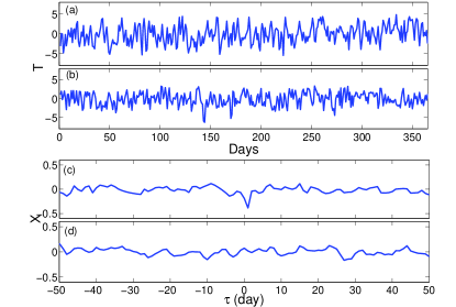
We implemented the above procedure for winter and summer time series, separately. Specifically, we calculate the cross-correlation functions of each pair of sites, where the data ranges from May 1st to Aug. 31st (123 days) for southern hemisphere (SH) winter (northern hemisphere, (NH) summer) or from Nov. 1st to Feb. 28th (120 days) for SH summer (NH winter). We choose a maximal time lag of 72 days and a time period of $y\in[1948,2010]$. The correlation coefficient and the link weight are based on 12 months of data, in order to have sufficient statistics. This is done by “gluing” together three consecutive winters (summers), such that the total number of months is 12.

Figure 2: (Color online) (a) The probability density function (PDF) of the mean weight of negative links in the globe, in both real (blue solid line) and shuffled (red dashed line) data. (b) The dependence of the standard deviation of time delay $\tau^{*}$ on the mean weight $\langle W\rangle$ for all possible links, for real (blue) and shuffled (red) data. (c) The mean negative link weight as a function of distance $d$, for the SH (blue circles), NH (red squares) and the equator (pink diamonds) regions. The figure is based on the globe temperature records at 1000 hPa isobar for Nov. to Feb..

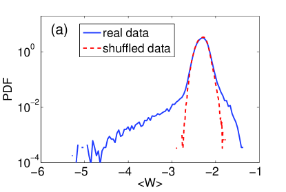
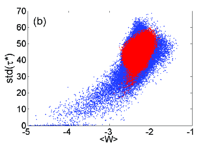
We analyze a near surface (1000 hPa) temperature time series. First, we focus on the properties of link weight around the globe (Fig. 2) for the months Nov. to Feb.. To identify the significant links we apply a shuffling procedure in which the order of the years is shuffled while the order within each year remains unchanged. This shuffling scheme is aimed at preserving all the statistical quantities of the data, such as the distribution of values, and their autocorrelation properties, but omitting the physical dependence between different nodes. Fig. 2(a) and (b) depict the link weight statistics for the real and shuffled data. High negative mean link weight values exist in the probability density function (PDF) of the real data but are missing in the shuffled data, and therefore are not likely to occur by chance. Moreover, high variability (std.) during different years of the time delays of links $\tau^{*}$ is also a signature of random behavior Bashan2012 (Fig. 2(b)). The differences between the distribution of real data and shuffled data indicate that many significant negative links exist in the climate network (Fig. 2(a),(b)). We obtain similar results for positive links and other fields (not shown).

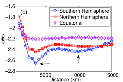
Next, we divide the world into three geographical zones, the SH (from 22.5^∘S to the south pole), the NH (from 22.5^∘N to the north pole) and the equator (between 22.5^∘S and 22.5^∘N). We then calculate the (geographical and temporal) mean link weight $\langle W_{s_{1},s_{2}}\rangle$ as a function of the geographical distance of links, $d$. It is clear that in the SH, there is a preferred distance of $\sim$ 3,500 km and a much weaker one of $\sim$ 10,000 km (Fig. 2(c)). In the NH region, we find a similar, weaker dependence, while in the equatorial region, there is no preferred distance (Fig. 2(c)). These preferred distances may be associated with atmospheric Rossby waves Chang2005 ; Chang1999(1) ; Chang1999 ; Chang1993 , which have a wavelength of $\sim$ 7,000 km and which are known to be pronounced in the SH, weaker in the NH and absent in the equatorial region Chang1999(1) ; Chang1999 . The negative peaks at 3,500 km and 10,000 km represent a 1/2 wavelength and a 3/2 wavelength of the observed Rossby wavelength.

Figure 3: (Color online) The dependence of the weight of negative links on the distance $d$ in the SH during (a) winter and (b) summer months. (c),(d) Same as (a),(b) for positive links. The PDF of time delays $\tau^{*}$ of near negative (blue squares, $d\sim$ 3,500 km), far positive (red circles, $d\sim$ 7,000 km), and far negative (pink diamonds, $d\sim$ 10,000 km) weighted links, in the SH during (e) winter and (f) summer. The figure is based on the temperature field at 1000 hPa isobar.

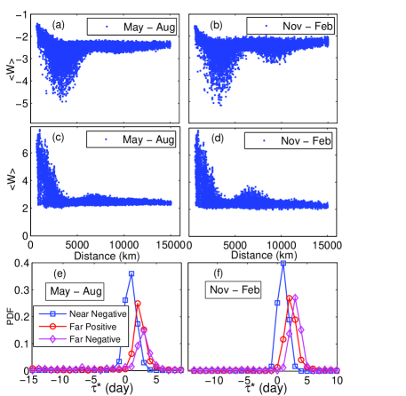
To further consolidate the association of the observed pattern in the climate network with Rossby waves, we compare the seasonality of this pattern with the known seasonal characteristics of Rossby waves. In Fig. 3(a)-(d), we plot the negative and positive weights of all SH links, for the winter and summer months separately. Each point represents an average link weight $\langle W\rangle$ over years versus its distance $d$. The negative weights, defined in Eq. (2), have a pronounced enhanced distribution of large weights for $d\sim$ 3,500 km during both summer and winter months, while for the SH summer months (Nov. to Feb.), there is an additional preferred distance of $\sim$ 10,000 km (Fig. 3 (b)), both in accordance with the 1/2 and 3/2 wavelengths of atmospheric Rossby waves. Around the full wavelength distance (i.e., $d\sim 7,000$ km), we find, as expected, an enhanced distribution of large positive weights (defined in Eq. (1)) (Fig. 3 (c),(d)). However, a larger abundance of strong waves (represented by links at 1/2, 1, and 3/2 wavelengths) during summer, in comparison to winter months, is clearly seen in Fig. 3 (a)-(d), in agreement with the clearer pattern of Rossby waves found during the SH summer in the SH Chang1999(1) ; Chang1999 ; Chang1993 . The situation is similar in the NH (not shown), for the NH winter. In the distribution of positive weights (Fig. 3(c),(d)), one clearly sees the links that emerge around $d<2,000$ km due to the proximity effect mentioned in the introduction.

Atmospheric Rossby waves have a characteristic group velocity, and we now estimate it based on the climate network results shown above. To achieve this, we divide $d$ by $\tau^{*}$ for each link, under the assumption that $\tau^{*}$ is a good estimate for the underlying dynamical delay between the two sites (nodes) cimp . Since $\tau^{*}$ is only meaningful for links with weights above the background noise level (see Fig. 2(b), and ref. Berezin2012 ), we limit the analysis to links with weights $|\overline{W}|>2.8$  fn1 . Furthermore, to avoid links that are prone to the proximity effect (as such links cannot easily fit in the current Rossby wave interpretation), when considering positively correlated links, we consider links with $d>5,000$ km. Also, we constrain the near negative links to be within $d\in[2,000km,5,000km]$ and far negative links to have $d>8,000$ km. The PDFs of time delay $\tau^{*}$ of the near negative links, the far positive links and the far negative links are shown in Fig. 3(e),(f). By our convention, positive $\tau^{*}$ means an eastward energy flow, which is the typical case for most observed links. The results point to a time lag of $\tau\approx$ 1 day for the near negative links (i.e., links in the first peak in Fig. 3(a)), $\tau\approx$ 2-3 days for the far (beyond the proximity effect) positive links, and $\tau\approx$ 3-4 days for the far negative links (i.e., belonging to the second peak in the scatter plot of Fig. 3(a,b)). Based on these numbers, our estimated group velocities are in the range $[20-35]$m/s, consistent with the range $[23-32]$m/s reported in previous studies Chang1999 ; Berbery1996 .

Figure 4: (Color online) The out- (a) and in-degree (b) of the climate network structure from Nov. to Feb. (SH summer). The out- (c) and in-degree (d) of the climate network structure from May to Aug. (SH winter). The figure is based on the temperature record at 1000 hPa isobar.

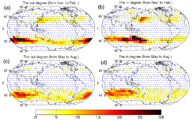
The climate network has a unique geographical structure that can be compared with the geographical structure of Rossby waves. Since the network is directed—positive $\tau$ indicates eastward flow while negative $\tau$ indicates westward flow—we distinguish between a link that is pointing toward a node (where the number of links pointing to a specific node is referred to below as “in-degree”), or away from the node (referred to below as “out-degree”) (see  Gozolchiani2011 ). Fig. 4 depicts the mean in- and out-degrees of each node, excluding the equatorial region that conforms with a pattern that is not related to our current discussion. The observed structure is consistent with the structure of Rossby waves Chang1999 . First, the wave band in the SH from May to August (SH winter, Fig. 4(c),(d)) is broader than that of the SH summer (Nov. to Feb., Fig. 4 (a,b)). Second, the atmospheric Rossby wave structure in the NH summer is less pronounced. Third, the wave structure in the SH summer (Nov. to Feb.) lies on a band centered near 50^∘S. All the above characteristics are consistent with the properties of Rossby waves.

Figure 5: (Color online) The dependence of the weight of negative links on the distance $d$ in the SH during SH summer months for temperature (left panels) and meridional velocity (right panels) for 300 hPa (upper panels) and 1,000 hPa (lower panels).

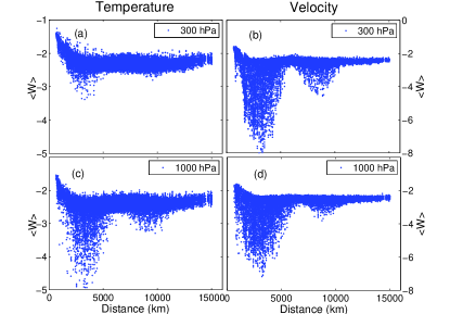
Previous studies found the 300 hPa meridional velocity field to be the most suitable for studying the characteristics of Rossby waves Chang1993 ; Chang1999 ; Chang1999(1) . Our method captures the wave properties also using other fields at various altitudes. In particular, we showed above that the wave pattern is clearly seen at a ground level (1000 hPa) temperature field, a more common and reliable variable. In Fig. 5, we compare, using the climate network technique, between the mean weight distributions of the negative links of the meridional velocity and temperature fields. We find that the pattern of the two fields is similar, although the meridional velocity yields larger weights. In addition, the meridional velocity yields a clearer pattern at the high altitude of 300 hPa, while the temperature field yields a clearer pattern at the ground level of 1000 hPa.

In summary, we analyze the properties of the climate network by considering, separately, positive and negative correlations (links). The most dominant links in the climate network with a geographical distance larger than 2,000 km are found for distances of $\sim$ 3,500 km, $\sim$ 7,000 km and $\sim$ 10,000 km. These distances coincide with the 1/2, 1 and 3/2 wavelengths of common atmospheric Rossby waves. Moreover, the time delays associated with these distances are in agreement with the direction of the energy flow and with the group velocity of the atmospheric Rossby waves. The pronounced length scales of the climate network, the dominance in the SH in comparison with the NH, and the dominance during the SH summer in the SH are all consistent with the properties of atmospheric Rossby waves. All of these factors thus provide strong support for the association of the majority of the climate network far links with Rossby waves.

References

- (1) R. Albert, A-L. Barabasi, Rev. Mod. Phys., 74, 47 (2002).
- (2) S. Boccaletti, V. Latora, Y. Moreno, M. Chavez and D-U. Hwang, Physics Reports, 424, 175 (2006).
- (3) M. E. J. Newman, Networks: An Introduction. Oxford Press, (2010).
- (4) R. Cohen and S. Havlin, Complex Networks: Structure, Robustness and Function, Cambridge University Press, (2010).
- (5) M. Girvan and M. E. J. Newman, Proc. Natl. Acad. Sci., U.S.A. 99, 7821 (2002).
- (6) R. Guimera and L. A. N. Amaral, Nature, 433, 895 (2005).
- (7) G. Palla, I. Derenyi, I. Farkas, and T. Vicsek, Nature, 435, 814 (2005).
- (8) H. Jeong, B. Tombor, R. Albert, Z. N. Oltvai, A.-L. Barabasi, Nature, 407, 651 (2000).
- (9) B. A. Huberman, The Laws of the Web, MIT Press, Cambridge, MA (2001).
- (10) A. Bashan et al., Nature Communications, 3, 702 (2012).
- (11) C. M. Schneider, A. A. Moreira, J. S. Andrade Jr, S. Havlin, H. J. Herrmann, Proc. Nati. Acad. Sci., U.S.A. 108, 3838 (2011).
- (12) A. A. Tsonis, K. L. Swanson, and P. J. Roebber, Bull. Am. Meteorol. Soc., 87, 585 (2006).
- (13) K. Yamasaki, A. Gozolchiani, and S. Havlin, Phys. Rev. Lett., 100, 228501 (2008).
- (14) A. A. Tsonis and K. L. Swanson, Phys. Rev. Lett., 100, 228502, (2008).
- (15) J. F. Donges, Y. Zou, N. Marwan and J. Kurths, Europhys. Lett., 87 48007, (2009).
- (16) Y. Berezin et al., Nature Scientific Reports, 2, 666 (2012).
- (17) A. Gozolchiani, S. Havlin and K. Yamasaki, Phys. Rev. Lett., 107, 148501, (2011).
- (18) O. Guez et al., Eurphys. Lett., 98, 38006 (2012).
- (19) J. F. Donges, Y. Zou, N. Marwan, and J. Kurths, Eur. Phys. J. Special Topics, 174, 157 (2009).
- (20) H. V. Storch and F. W. Zwiers, Statistical Analysis in Climate Research, Cambridge University Press, (2003).
- (21) L. F. Robinson, V. H. de la Pena and Y. Kushnir, Theoretical and Applied Climatology, 94, 215 (2008).
- (22) P. Alpert and T. Sholokhman, Factor Separation in the Atmosphere: Applications and Future Prospects, Cambridge University Press, (2011).
- (23) J. M. Wallace and D. S. Gutzler, Mon. Wea. Rev., 109, 784 (1981).
- (24) B. J. Hoskins and D. Karoly, J. Atmos. Sci., 38, 1179 (1981).
- (25) G. T. Walker, Quarterly Journal of the Royal Meteorological Society, 51, 337 (1925).
- (26) E. K. M. Chang, J. Atmos. Sci., 62, 2467 (2005).
- (27) E. K. M. Chang, J. Atmos. Sci., 50, 2038 (1993).
- (28) E. K. M. Chang, and B. Y. Daniel, J. Atmos. Sci., 56, 1708 (1999).
- (29) E. K. M. Chang, J. Atmos. Sci., 56, 1729 (1999).
- (30) Kalnay et al., Bull. Amer. Meteor. Soc., 77, 437-470, (1996). http://www.esrl.noaa.gov/psd/data/gridded/
- (31) The original resolution of the reanalysis data is 2.5∘. The number of nodes that were analyzed was normalized by the cosine of latitude, to keep the density of nodes equally distributed.
- (32) L. Cimponeriu, M. Rosenblum and A. Pikovsky, Phys. Rev. E, 70, 046213 (2004)
- (33) We have checked thresholds in the range without significant qualitative changes in the results.
- (34) E. H. Berbery, and C. S. Vera, J. Atmos. Sci., 53, 468 (1996).