TU-933
Isocurvature Constraints and Anharmonic Effects
on QCD Axion Dark Matter
Takeshi Kobayashi,a,b111takeshi@cita.utoronto.ca,
Ryosuke Kurematsu,c222rkurematsu@tuhep.phys.tohoku.ac.jp
and Fuminobu Takahashic333fumi@tuhep.phys.tohoku.ac.jp
aCanadian Institute for Theoretical Astrophysics,
University of Toronto,
60 St. George Street, Toronto, Ontario M5S
3H8, Canada
bPerimeter Institute for Theoretical Physics,
31 Caroline Street North, Waterloo, Ontario N2L 2Y5, Canada
c Department of Physics, Tohoku University, Sendai 980-8578, Japan
1 Introduction
The identity of dark matter is one of the central issues in cosmology and particle physics. The QCD axion is an interesting and plausible candidate for dark matter; it is a Nambu-Goldstone (NG) particle associated with the spontaneous breakdown of the Peccei-Quinn (PQ) symmetry introduced to solve the strong CP problem in QCD [1, 2]. As the axion settles down at the potential minimum, the CP violating phase is set to a vanishingly small value, solving the strong CP problem.
The dynamical relaxation of the CP phase necessarily induces coherent oscillations of the axion, which contribute to dark matter, since the axion is stable in a cosmological time scale for the decay constant in the axion window [3],
| (1) |
The lower bound comes from astrophysical constraints including the cooling argument of globular-cluster stars, and the upper bound from the requirement that the axion density should not exceed the observed dark matter density for the initial misalignment angle of order unity. If the fine-tuning of the initial position is allowed, or if non-standard cosmology is assumed [4], the upper bound can be relaxed to e.g. the GUT or string scale.
One of the features of the axion is that its quantum fluctuation during inflation naturally induces an almost scale-invariant isocurvature density fluctuation, which would leave a distinctive imprint on the CMB spectrum.444 If the QCD interactions become strong at an intermediate or high energy scale in the very early Universe, the axion may acquire a sufficiently heavy mass, leading to suppression of the isocurvature perturbations [5]. The observed CMB spectrum is known to be fitted extremely well by a nearly scale-invariant adiabatic density perturbation, and a mixture of the isocurvature perturbations is tightly constrained by the observations [6, 7]. This constraint can be interpreted as an upper bound on the inflation energy density as the quantum fluctuation of the axion field is set by the Hubble parameter during inflation [8, 9].
The statistical information contained in the density fluctuations can be exploited by estimating higher order correlation functions. The non-Gaussianity of the isocurvature density fluctuations has been studied from both theoretical [10, 11, 12, 13, 14] and observational [15, 16, 17] point of view. In particular, the non-Gaussianity of the CDM isocurvature perturbation induced by the axion was estimated under an approximation assuming a quadratic potential for the axion [10]. This approximation however breaks down as the initial misalignment angle deviates from the CP symmetric vacuum, and an anharmonic effect must be taken into account. The anharmonic effect on the axion abundance and the isocurvature power spectrum was studied in Refs. [18, 19, 20, 21, 22]. However, while there is a consensus on the anharmonic effect on the axion abundance, there are apparent disagreement as to how the isocurvature perturbations are affected by the anharmonic effect.
Recently an analytic method and approximations to compute density perturbations induced by a curvaton field with a broad class of the potential was developed by Kawasaki and two of the present authors (Kobayashi and Takahashi) (KKT in the following) [23]. Using this new method, we can analytically estimate the density perturbations generated in a curvaton mechanism [24, 25, 26, 27] for a potential significantly deviated from the simple quadratic one [23, 28, 29].555 In the hilltop limit, the density fluctuations receive a dominant contribution from the fluctuations of the timing when the curvaton starts to oscillate, rather than from those of the oscillation amplitude, in contrast to what is usually assumed for the quadratic potential. To our knowledge, this observation was first made in Ref. [30], and its analytic understanding was developed in Ref. [23]. See also Ref. [31] for spectator field models in light of the spectral index after the Planck. The analytic and numerical results were found to agree with each other to a very good accuracy, typically, within several percent. This method was however limited to a time-independent potential for the curvaton.
In this paper we extend the analytic method to a time-dependent potential, and then apply the method to the case of the QCD axion. We find it essential to define the onset of oscillations properly in order to evaluate the axion isocurvature perturbations. To this end we solve an attractor equation of motion for the axion until it starts to oscillate. This is the key to understand the anharmonic effect on the behavior of isocurvature perturbations. Based on the extended KKT method, we first correctly estimate the power spectrum and non-Gaussianity of the axion isocurvature perturbations for any axion initial position, resolving the aforementioned disagreement in the literature. We find that both power spectrum and non-Gaussianity are enhanced as the initial field value approaches the hilltop of the potential, thus giving an extremely tight constraint on the inflation scale for the axion decay constant GeV, near the smaller end of the axion dark matter window (1). We will also provide useful formulae for the power spectrum and non-Gaussianity of the axion isocurvature perturbations.
Here let us summarize the comparison of our results with the works in the past. First of all, the axion abundance has been studied extensively in the past, including the hilltop limit, and we obtained results which are consistent with the previous works. Namely, the axion abundance is enhanced as the initial field value approaches the hilltop of the potential. However, concerning the power spectrum of the axion isocurvature perturbations, we find that there are some inconsistencies among the literature. As we shall see later, we find that the power spectrum of the axion isocurvature perturbation gets significantly enhanced toward the hilltop, and its behavior agrees well with the result of Ref. [19] valid near the hilltop. However, such an enhancement was not correctly taken into account in Ref. [22], which resulted in a much weaker constraint on the inflation scale for GeV in their Fig. 1. In Ref. [32], it was pointed out that the power spectrum can be suppressed or enhanced by the anharmonic effects depending on the parameters. We do not confirm such suppression in our analysis. Furthermore, their enhancement factor is weaker than what we find.
The rest of this paper is organized as follows. In Sec. 2 we summarize the basic properties of the QCD axion. In Sec. 3, we give a brief review of the recently developed analytic approach and extend it to include the time-dependent potential. We apply this analysis to the QCD axion, and calculate the derivative of the e-folding with respect to the axion field value at the horizon exit. In Sec. 4, using the results in Sec. 3, we estimate the power spectrum and non-Gaussianity of the isocurvature perturbations, and derive constraints on the inflation scale as a function of the axion decay constant. We also provide useful formulae for the power spectrum and non-Gaussianity of the axion isocurvature perturbations; given the analytic expression for the axion dark matter abundance, one can easily estimate them using the formulae. The last section is devoted to conclusions.
2 Axion Dark Matter
We here briefly review the basics of the QCD axion dark matter. The axion is a NG boson associated with the spontaneous breaking of the PQ symmetry, which was introduced to solve the strong CP problem. Throughout this paper we assume that the PQ symmetry is already broken during inflation and is not restored after inflation666 The isocurvature perturbations are not generated if the PQ symmetry is restored during or after inflation [33, 34]. In this case, however, the topological defect such as the cosmic strings and domain walls are generated, and in particular, the PQ sector must be such that the domain wall number is unity. , and that the PQ breaking scale remains unchanged during and after inflation. See Ref. [35, 36] for the case where the PQ breaking scale, and therefore the coefficient of the kinetic term for the axion, significantly evolves after inflation, which would suppress/enhance the axion quantum fluctuations. A similar effect is possible if there is a non-minimal coupling to gravity [37]. It is also possible to make the axion so heavy during inflation that its quantum fluctuations are suppressed if the QCD becomes strong at an intermediate or high energy scale [5].
The axion has a flat potential protected by the PQ symmetry, which however is explicitly broken by the QCD anomaly. Thus, as the comic temperature drops down to the QCD scale, MeV, the QCD interactions become strong and non-perturbative, and the axion gradually acquires a finite mass from the QCD instanton effects. The axion potential is approximately given by
| (2) |
where is the axion decay constant and is the temperature dependent axion mass approximately given by [38]
| (5) |
with and . We set the CP symmetric vacuum to be the origin of the axion. The axion mass at zero temperature is related to the decay constant as
| (6) |
where , MeV, MeV, and we used the conventional value for in the second equality.
At a sufficiently high temperature, the axion mass is much smaller than the Hubble parameter. When the temperature becomes as low as GeV, the axion starts to oscillate around the potential minimum. Throughout this paper we assume the radiation dominated Universe when the axion starts to oscillate. For a small initial misalignment angle, , the axion potential can be approximated with a quadratic potential. Then the axion abundance is given by
| (7) |
where is the present-day Hubble parameter in units of km s-1 Mpc-1. One can see from this form that the observed dark matter abundance can be naturally explained by the coherent oscillations of the axion for the initial misalignment angle of order unity and for . On the other hand, the initial misalignment angle must be finely tuned to be an extremely small value for to avoid the overclosure of the Universe.
If the axion field initially sits near the maximum of the potential, i.e., , the commencement of the coherent oscillations can be significantly delayed. This is known as the anharmonic effect [18, 19]. In the following we study its effect on the isocurvature fluctuations of the axion by using the recently developed analytic method. We shall see that the anharmonic effect leads to the enhancement of the abundance as well as the isocurvature perturbations of the axion.
3 Analytical method of density perturbations
3.1 Basic strategy
Here we provide a basic strategy of the analytical method to compute the density perturbations generated by quantum fluctuations of a scalar field. See Ref. [23] for details.
The density perturbations induced by a light scalar field depend on the scalar evolution during and after inflation. Suppose that the scalar potential is approximated by a quadratic potential, and that its mass is sufficiently light during and for some time after inflation. Then the scalar field hardly evolves and stays more or less at the initial position until it starts to oscillate. When the Hubble parameter becomes comparable to the mass, it starts to oscillate, and importantly, the timing does not depend on the position. This is no longer the case for a potential of the general form, and one needs to follow the evolution of the scalar field until the commencement of coherent oscillations in order to compute the density perturbations. To this end, we first note that the scalar evolution can be actually well described by an attractor equation of motion. Then, by using the attractor equation of motion, we express the dependence of the e-folding number on the initial position of the scalar field. Finally we compute the power spectrum and non-Gaussianity parameter of the isocurvature perturbations, making use of the -formalism [39, 40, 41, 42]. The most important ingredients are and , where is the e-folding number between the horizon exit and some time after the matter-radiation equality, and is the field value at the horizon exit of the CMB scales. The purpose of the rest of this section is to express and in terms of the scalar potential and the axion field.
In Ref. [23], the scalar potential was assumed to be time-independent. Here we shall extend the attractor equation of motion to include a possible time-dependence of the scalar potential, which is an essential feature of the axion.
3.2 The attractor equation of motion
Here we derive an attractor equation of motion of the following form,
| (8) |
where is a positive constant, a dot represents a -derivative, and a prime a partial differentiation with respect to the scalar field . In the following discussion we identify with the QCD axion, but most of the results in this section can be straightforwardly applied to a generic scalar field with a potential with explicit time dependence.
The attractor equation for a time-independent potential was derived in Ref. [43] and also in Appendix A of Ref. [23]. The point is that, the scalar evolution can be well described by a first order differential equation when the curvature of the potential is much smaller than the Hubble parameter. The coefficient is determined so that the attractor equation is consistent with the true equation of motion, .
To simplify our analysis we consider a potential of the form, , with , where is a constant. Then the constant in (8) should satisfy
| (9) |
This shows that in a Universe with constant (i.e. constant equation of state parameter ), then as long as that the potential curvature is as small as , the constant is given by
| (10) |
One can further check that the approximation (8) with (10) is actually a stable attractor for .
In the case of axion, the temperature dependence is given by777 We have confirmed that such approximation is indeed valid until the commencement of oscillations for the parameter region of our interest. For example, the axion mass can approach its zero-temperature value before the axion starts to oscillate if the axion is located extremely close to the hilltop (beyond the region studied in this paper), however in such case the axion density would exceed the observed dark matter density.
| (11) |
for . This leads to
| (12) |
i.e., , where we have assumed radiation-domination, , in the second equality.888The temperature dependence of the relativistic degrees of freedom is neglected in the second equality of (12). We remark that within the temperature range where the axion starts its oscillations, changes slowly enough such that its time variation gives at most % modification to the value of . (Having a constant greatly simplifies the analysis for axions, as we will soon see.) The coefficient can be approximated with
| (13) |
where we used . The attractor equation of motion will be valid as long as
| (14) |
Roughly speaking, the attractor equation of motion holds until the curvature of the potential becomes about times as large as the Hubble parameter.
3.3 The onset of oscillations
The early stage of the scalar evolution can be described well by the attractor equation, which however breaks down at a certain point, and the scalar field starts to oscillate around the potential minimum. The purpose of this subsection is to define the timing of the commencement of oscillations, , or equivalently, , and to calculate its dependence on the initial position . Specifically, we will calculate and .
Setting the potential minimum around which the scalar oscillates to , the oscillations are considered to start when
| (15) |
where is a constant of order unity. We will set it to be unity in the numerical calculations, but we have confirmed that our results remain almost intact as long as is of order unity. Combined with the attractor equation, we obtain
| (16) |
where it is assumed that the potential is an increasing function of from the origin to the field values of interest. Differentiating both sides with respect to , we obtain
| (17) |
where and , and it should be noted that the potential explicitly depends on the time, which also depends on . (In other words, and are related through Eq. (15).) Using
| (18) |
which holds in the radiation dominated era, we obtain
| (19) |
with
| (20) |
For later use we rewrite Eq. (19) as
| (21) |
If the scalar potential is quadratic, the function vanishes. On the other hand, in the hilltop limit, becomes much larger than unity. Thus, is considered to represent the effect of the deviation of the scalar potential from a quadratic one.
Next we calculate . Integrating the attractor equation over and , we obtain
| (22) |
where actually means , and terms that are independent of are denoted as const. We differentiate both sides with respect to to obtain
| (23) |
The main results of this subsection are (19) and (23), which will be used later to calculate .
3.4 Axion number density
Next we estimate the axion number density. Since the axion mass increases after the onset of oscillations, it is the number density that determines the relic abundance of the axion; the number density decreases in proportional to the inverse of the volume, and its ratio to the entropy density is fixed. The axion energy density at a later time can be estimated by multiplying the number density with the zero-temperature mass, .
Denoting the mass at the origin on the onset of oscillations as , the number density is related to the potential and mass as
| (24) |
Precisely speaking, the number density is also dependent on the kinetic energy. However, one can see that the kinetic energy contribution becomes smaller as one goes to the hilltop region, since the onset of oscillations are delayed. This can be seen as follows. The kinetic energy can be estimated as
| (25) |
where (15) is used. On the other hand, the potential energy is
| (26) |
Thus, for the delayed onset of oscillations, , the kinetic energy is smaller than the potential energy.
Differentiating the number density with respect to , one obtains
| (27) | |||||
where it should be noted that has no explicit dependence on , and so, . Using and Eq. (21), one arrives at
| (28) |
3.5 The e-folding number
Now we are ready to calculate the derivative of the e-folding number with respect to , which is directly related to the primordial curvature perturbations in the formalism. We are interested in the e-folding number between the horizon exit of the cosmological scales and some time after the matter-radiation equality, and these times are represented by and . Specifically we take the slicings at and as the flat slicing and uniform density slicing, respectively. The e-folding number between and is given by
| (29) |
Let us split the integral into two pieces;
| (30) | |||||
| (31) |
It is useful to use the radiation energy density, or the entropy density, instead of the time. We adopt the entropy density, , which scales as the inverse of the volume, even if the relativistic degrees of freedom changes with time;
| (32) |
The e-folding numbers can be rewritten as
| (33) |
where and , and the constant term in does not depend on . The radiation energy density is related to the entropy density as
| (34) |
We are interested in the derivative of the e-folding number with respect to . The variation of , , is set by the Hubble parameter during inflation, , and the corresponding fractional change of the temperature, , is much smaller than unity for the parameters of our interest. Thus, we can practically neglect the change of and due to the variation of . Similar discussions apply to and as well. Then we obtain
| (35) | |||||
| (36) |
where we have assumed that the Universe was radiation-dominated and the axion and the other CDM components were negligible at . The advantage of using the entropy density is that it becomes clear that the above formulae are still valid even if the relativistic degrees of freedom changes between and .
Now we estimate the first term in Eq. (36), which turns out to be rather involved. To this end we define
| (37) | |||||
| (38) |
where the total DM density is given by , and denotes the CDM component other than the QCD axion. Using and , we have (note that on the final uniform density slicing is a constant that is chosen independently of )
We suppose that the entropy perturbation between and is not generated by the fluctuation of . (Hence we consider the CDM components other than the axion are produced while the axion has little effect on the expansion of the Universe.) Thus,
| (40) |
namely,
| (41) |
So, we obtain
| (42) |
Substituting this into Eq. (36), we arrive at
| (43) |
To summarize,
| (44) | |||||
where we used Eq. (19) and Eq. (28) in the last equality, and is understood as . This result is reasonable, since it vanishes in the limit of , i.e., when the axion has negligible energy density.
In order to estimate the non-Gaussianity of the isocurvature perturbations, we need to calculate . The following formulae are useful for this purpose;
| (45) | |||||
| (46) |
which can be shown by direct calculation. After long calculation, we obtain the second derivative of as
Now we are ready to estimate the isocurvature perturbations and its non-Gaussianity.
4 The axion isocurvature perturbations and its non-Gaussianity
4.1 Power spectrum and bi-spectrum
Let us start by discussing how the two-point and three-point correlation functions of the isocurvature perturbations can be expressed in the formalism [39, 40, 41, 42], following Ref. [10].
The isocurvature perturbation is defined as
| (49) |
where is the curvature perturbation on the slicing where the dark matter (radiation) is spatially homogeneous. Using the formalism, is obtained as the fluctuations in the number of e-folds between an initial flat slicing (which we take as the time of CMB scale horizon exit) and a final uniform- slicing, among different patches of the Universe. Since we are interested in the difference between and , we only need to compute the contribution to arising from the axion field fluctuations . Thus (49) can be expressed in terms of the derivative of the e-folding number as [10]999Here we do not consider fluctuations of CDM components other than the axion, and further suppose that there are no mixing terms such as where is the inflaton field.
| (50) |
By taking the final uniform- slicing for to be deep in the matter dominated era, i.e., , the slicing can be identified with a uniform total density slicing and thus we can use the results from the previous section.101010We should remark that baryons are not taken into account throughout this paper. The simplified treatment is sufficient for giving order-of-magnitude constraints on the axion and inflationary parameters. Here let us also note that baryons can be added to the above analyses by extending the density ratios defined in (37) and (38) by (51) with denoting the total matter (= CDM + baryons) density. However obtained in this way with the choice of a final uniform- slicing would give isocurvature perturbations between radiation and total matter.
One may wonder about the validity of using the formalism since the CDM and radiation components exchange energy with each other, as is clearly seen from the explicit temperature dependence of the axion mass. Here we remark that after the interactions are turned off, the perturbations can be computed as the between flat and uniform- slicings. Moreover since the Universe expands uniformly between flat slicings, the initial flat slicing can be chosen arbitrarily, which we take it to be when the CMB scale exits the horizon as we can use the usual estimate for field fluctuations .
The power spectrum and the bispectrum are usually defined in the momentum space as
| (52) | ||||
| (53) |
where the isocurvature perturbation in the momentum space is defined by
| (54) |
The momentum dependence of the bispectrum can be approximately factored out;
| (55) |
where is the non-linearity parameter for the isocurvature perturbations.111111 is identical to used in Ref. [10].
Similarly we define the power spectrum of the axion field fluctuations;
| (56) |
where
| (57) |
The power spectrum and the non-linearity parameter of the isocurvature perturbation can be expressed as, to leading order in the field fluctuations,121212 It is straightforward to take into account of higher-order contributions, which can be relevant if is not sufficiently small compared to . This is the case if one considers a large value of and/or a small value of . Note however that the expansion of in terms of breaks down for . When the potential can be approximated by a quadratic one, an order-of-magnitude estimate of is still possible by simply replacing with , where .
| (58) |
where we consider the axion to have Gaussian field fluctuations. Let us repeat that in the above expressions, we substitute the results from the previous section deep in the matter-dominated era, i.e., .
The constraint from the Planck and the WMAP large-scale polarization data reads [7]
| (59) |
where represents the relative amplitude of the power spectrum of the isocurvature perturbation to that of the adiabatic one:131313 Note that defined here corresponds to in Ref. [7].
| (60) |
with Mpc-1. The power spectrum of the curvature perturbations is given by [44]
| (61) |
The bound on the non-linearity parameter was derived using the WMAP 7-yr data [16],
| (62) |
for the scale-invariant isocurvature perturbations, assuming the absence of non-Gaussianity in the adiabatic perturbations.141414 We expect that the constraint on can be improved considerably by using the Planck data.
4.2 Axionic isocurvature perturbations and its non-Gaussianity
Now we are ready to obtain the analytical expression for the isocurvature perturbation and its non-Gaussianity generated by the axion, by combining the results in the preceding sections.
Let us first calculate the power spectrum of the isocurvature perturbation. To simplify the expression, we define . Using Eq. (44), we then obtain
| (63) |
where we have taken the limit of . Here, recall that is a constant of order unity, , and is given as
| (64) |
In the hilltop limit, (cf. (20)) becomes much larger than unity, and both and approach . Actually, however, decreases much more slowly than [23]. Thus, the power spectrum of the isocurvature perturbation gets enhanced significantly by the factor , in the hilltop limit. Note that is also enhanced in the hilltop limit (see Fig. 1), which is much milder compared to the enhancement due to the factor .
The non-Gaussianity parameter is given by
| (65) | |||||
In contrast to the power spectrum, there is no huge enhancement due to in the hilltop limit; the increase of is much milder and is mainly due to . Note also that does not depend on the inflation scale, while the power spectrum does.
In order to see the consistency of the above result with the previously known results, let us consider a quadratic potential, for which and . This corresponds to the case where the initial misalignment angle is small. Then one can easily check
| (66) |
in the limit of the quadratic potential, . This coincides with the result, for in Ref. [10].
Using the above relations (63) and (65), let us estimate the isocurvature perturbations and its non-Gaussianity of the axion dark matter. To this end, we need to solve Eq. (15) (or Eq. (22)) in order to evaluate the commencement of oscillations, which determines , as well as . We have numerically solved the equation of motion for the axion in a radiation dominated Universe and obtained from Eq. (15), then substituted to the above relations to obtain and . The ratio is also numerically computed in order to obtain . We present these semi-analytic results in the following.
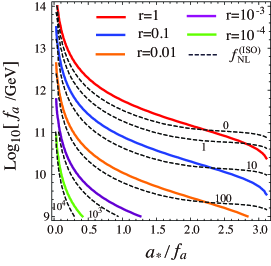
In Fig. 1, we show the contours of the fraction of the axion to the total dark matter density, (see Eq. (38)), and the non-linearity parameter , in the plane of the initial misalignment angle and the axion decay constant . In the region above the top (red) solid line, the axion abundance exceeds the observed dark matter abundance. We can see that, for a given value of , the axion abundance increases as the initial position approaches the hilltop, . Accordingly, the observed dark matter abundance is realized at a smaller value of for the hilltop initial condition, . The contours of show that they are parallel to those of for . This is because, as we have seen above, is determined simply by when the scalar potential can be approximated with the quadratic potential. On the other hand, as the initial position approaches the hilltop, the value of mildly increases along the contours of . This mild increase is due to the delayed onset of oscillations, which is one of the features of the hilltop curvaton [23].
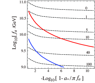
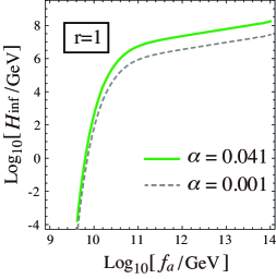
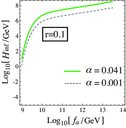
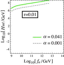
The inflationary scale, , is bounded from above by the isocurvature constraint (59). The contours of the upper bound on are shown in Fig. 2. Since the isocurvature perturbation is significantly enhanced towards the hilltop, the constraint on becomes tight. For instance, for , must be smaller than GeV.151515We have checked that the axion does not fall into wrong vacuum by climbing over the hilltop of the potential due to the quantum fluctuations, as long as the isocurvature constraint on is satisfied. On the other hand, the non-Gaussianity constraint (62) gives much weaker constraints in the hilltop region. One can see this by noting that is at most in the hilltop when , leading to . If the axion is a tiny fraction of dark matter (say, ), the non-Gaussianity constraint becomes important, as shown in Ref. [10].
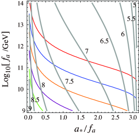
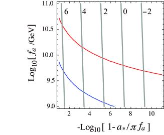
Lastly, we show the constraint on as a function of the decay constant in Fig. 3. For comparison, we show two constraints, , and . The first one represents the current constraints from the Planck and WMAP large-scale polarization data, while the latter one is just for showing how the constraint changes as the constraint on improves. We can see that the constraint becomes extremely tight for due to the anharmonic effect near the hilltop. The effect becomes milder as decreases since the initial misalignment angles deviates from the hilltop.
4.3 Useful expressions for and
In order to see if the above semi-analytic estimate correctly describes the power spectrum and non-Gaussianity of the axion isocurvature perturbations, let us compare them with another (more direct) calculation. To this end, it is important to note that (i) the actual abundance of the QCD axion is much smaller than that of radiation in the early times, which makes it extremely difficult to numerically solve the evolution of the QCD axion from its formation until the Universe becomes matter-dominated; (ii) in contrast to the ordinary curvaton scenario, the total dark matter abundance is fixed by observations. Namely, the abundance of the dark matter other than the QCD axion must be adjusted so that the total dark matter density satisfies . The condition for the adiabatic density perturbation, Eq. (40), fixes how to compensate the contribution of the QCD axion.
Let us recap how the isocurvature density perturbations are generated. The axion acquires quantum fluctuations of order , which results in the fluctuations of the axion density. The fluctuations of the e-folding number is through the isocurvature fluctuations of the dark matter density. Therefore, in principle, if we know how the axion density fluctuates and how the e-folding number fluctuates through the isocurvature fluctuations of the dark matter density, we should be able to estimate the isocurvature perturbation and its non-Gaussianity.
The present homogeneous or spatially averaged dark matter density should satisfy,
| (67) |
and it is that acquires spatial fluctuations, while is independent of . Note however that does depend on through (67), but its fluctuations do not on . More precisely speaking, the dependence of on arises from the requirement that the (spatially averaged) total dark matter density reproduce the observed value. However, its fluctuations is adiabatic and therefore independent of . Thus, when we expand the e-folding number with respect to , we should use
| (68) |
where and are energy densities on a flat slicing at an arbitrary time. Let us repeat that we are expanding w.r.t. the fluctuations , and for the expansions we need not consider the spatially averaged observational constraint (67).
Thus, we may evaluate as follows;
| (69) |
with
| (70) |
where we have used Eq. (68). Thus, the power spectrum and the non-Gaussianity are given by
| (71) | |||||
| (72) |
The exact solution for the evolution of the Universe which contains radiation and non-relativistic matter is parametrized in terms of a parameter as
| (73) | |||||
| (74) |
where is the scale factor (it should not be confused with the axion ), is a cosmological time, denotes the density parameter for radiation, and the subscript “” denotes values at an arbitrary time. In the matter-domination limit,
| (75) |
The uniform density slicing corresponds to a constant surface. Thus, taking both the initial flat slicing and final uniform density slicing to be in the matter-dominated era, the e-folding between them depends on on the initial slicing as161616The results in this page can also be derived from the following equation in the matter-dominated era: (76) where the energy densities in the left hand side are those on the initial flat slicing, is on the final uniform density slicing, and is the number of e-folds between the two slicings.
| (77) | |||||
| (78) |
giving
| (79) | |||||
| (80) |
Since both and redshift as , they can be replaced by energy densities on a flat slicing in the later Universe, and we finally obtain useful expressions for and :
| (81) | |||||
| (82) |
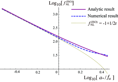
Thus, given the axion abundance as a function of , we can estimate the power spectrum as well as the non-Gaussianity parameter . (To be precise, the abundance in (81) and (82) is not the averaged quantity over the entire observed sky. Instead, it should be considered as a function of denoting how the present axion density responds to the initial axion field value. The critical density here is taken as a constant.171717Furthermore, the density ratio in (81) and (82) is that on a flat slicing, in contrast to in (38) defined on a uniform density slicing. However the two ’s are approximately the same and hence we do not distinguish them in the expressions for and .) If , these expressions reproduce the known results, , and (see (66)). Note that our analytic result for given in (65) is expressed in terms of the parameters at , while the above estimate (82) depends on the final axion abundance. The advantage of the analytic results in the previous subsection is that one can easily understand the behavior of the isocurvature perturbation and its non-Gaussianity in terms of the axion dynamics and the potential. On the other hand, the expression (82) is more useful when the (approximate) analytic expression for the axion abundance is known. It is also suitable for numerical calculations.
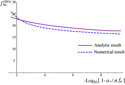
In Fig. 4, we compare two expressions for , (65) and (82), for GeV. They agree with each other well for a wide range of the initial condition within about %. We can also see that the expression is indeed valid only near the origin.
5 Conclusions
In this paper we have extended the analytic method developed by KKT to a time-dependent potential and then applied it to the QCD axion. We have derived the analytical expressions for the isocurvature power spectrum (63) and its non-Gaussianity parameter (65). Interestingly, the power spectrum significantly increases in the hilltop limit, while the non-Gaussianity increases only mildly. Specifically, becomes a few tens in the hilltop limit when the axion is the dominant component of dark matter. If the axion is a subdominant component of dark matter, it increases as in the non-hilltop region (see (66)). The upper bound on the inflation scale becomes extremely tight in the hilltop limit; GeV for when the axion is the dominant component of dark matter. (See Fig. 3). Our analytic expressions for the axionic isocurvature perturbations will be useful for a probe of the QCD axion dark matter by using the CMB data.
Acknowledgment
TK thanks Ramandeep Gill and Toyokazu Sekiguchi for helpful conversations. This work was supported by the Grant-in-Aid for Scientific Research on Innovative Areas (No.24111702, No. 21111006, and No.23104008), Scientific Research (A) (No. 22244030 and No.21244033), and JSPS Grant-in-Aid for Young Scientists (B) (No. 24740135) [FT]. This work was also supported by World Premier International Center Initiative (WPI Program), MEXT, Japan
Appendix A Another derivation of upper bounds on and evaluation of
Here let us estimate the isocurvature constraint on by using the analytic expression (81) and a known analytic approximation of the anharmonic effect. To this end, we use the axion abundance [21],
| (83) |
with the anharmonic coefficient [22]
| (84) |
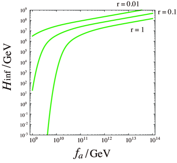
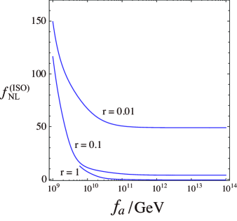
where we have changed the exponent so as to be consistent with the axion abundance, although this change does not affect our results. Substituting these into (81), we obtain the resultant isocurvature perturbation which is constrained by (59). We can express the constraint as an upper bound on as a function of for fixed (i.e., is given as a function of ). The result is shown in Fig. 5, where the upper bounds are shown for , and from bottom to top. We can see that the constraints are consistent with what we obtained by using the semi-analytic formulae (see Fig. 3). Similarly, we can evaluate by substituting the above expressions into (82). See Fig. 6. The enhancement toward the lower value of is due to the anharmonic effect represented by in (65).
References
- [1] R. D. Peccei and H. R. Quinn, Phys. Rev. Lett. 38, 1440 (1977); Phys. Rev. D 16, 1791 (1977).
- [2] For a review, see J. E. Kim, Phys. Rept. 150, 1 (1987); H. Y. Cheng, Phys. Rept. 158, 1 (1988); J. E. Kim and G. Carosi, Rev. Mod. Phys. 82, 557 (2010) [arXiv:0807.3125 [hep-ph]]; A. Ringwald, Phys. Dark Univ. 1 (2012) 116 [arXiv:1210.5081 [hep-ph]]; M. Kawasaki and K. Nakayama, arXiv:1301.1123 [hep-ph].
- [3] G. G. Raffelt, “Stars as Laboratories for Fundamental Physics,” Chicago University Press, USA (1996).
- [4] M. Kawasaki, T. Moroi and T. Yanagida, Phys. Lett. B 383, 313 (1996) [hep-ph/9510461].
- [5] K. S. Jeong and F. Takahashi, arXiv:1304.8131 [hep-ph].
- [6] G. Hinshaw, D. Larson, E. Komatsu, D. N. Spergel, C. L. Bennett, J. Dunkley, M. R. Nolta and M. Halpern et al., arXiv:1212.5226 [astro-ph.CO].
- [7] P. A. R. Ade et al. [ Planck Collaboration], arXiv:1303.5082 [astro-ph.CO].
- [8] D. Seckel and M. S. Turner, Phys. Rev. D 32, 3178 (1985).
- [9] D. H. Lyth, Phys. Lett. B 236, 408 (1990).
- [10] M. Kawasaki, K. Nakayama, T. Sekiguchi, T. Suyama and F. Takahashi, JCAP 0811, 019 (2008) [arXiv:0808.0009 [astro-ph]]; JCAP 0901, 042 (2009) [arXiv:0810.0208 [astro-ph]].
- [11] D. Langlois, F. Vernizzi and D. Wands, JCAP 0812, 004 (2008) [arXiv:0809.4646 [astro-ph]].
- [12] E. Kawakami, M. Kawasaki, K. Nakayama, F. Takahashi and , JCAP 0909, 002 (2009) [arXiv:0905.1552 [astro-ph.CO]].
- [13] D. Langlois, A. Lepidi and , JCAP 1101, 008 (2011) [arXiv:1007.5498 [astro-ph.CO]].
- [14] D. Langlois, T. Takahashi and , JCAP 1102, 020 (2011) [arXiv:1012.4885 [astro-ph.CO]].
- [15] C. Hikage, K. Koyama, T. Matsubara, T. Takahashi and M. Yamaguchi, Mon. Not. Roy. Astron. Soc. 398, 2188 (2009) [arXiv:0812.3500 [astro-ph]].
- [16] C. Hikage, M. Kawasaki, T. Sekiguchi and T. Takahashi, arXiv:1211.1095 [astro-ph.CO].
- [17] C. Hikage, M. Kawasaki, T. Sekiguchi and T. Takahashi, arXiv:1212.6001 [astro-ph.CO].
- [18] M. S. Turner, Phys. Rev. D 33, 889 (1986).
- [19] D. H. Lyth, Phys. Rev. D 45, 3394 (1992).
- [20] K. Strobl and T. J. Weiler, Phys. Rev. D 50, 7690 (1994) [astro-ph/9405028].
- [21] K. J. Bae, J. -H. Huh, J. E. Kim and , JCAP 0809, 005 (2008) [arXiv:0806.0497 [hep-ph]].
- [22] L. Visinelli, P. Gondolo and , Phys. Rev. D 80, 035024 (2009) [arXiv:0903.4377 [astro-ph.CO]].
- [23] M. Kawasaki, T. Kobayashi and F. Takahashi, Phys. Rev. D 84 (2011) 123506 [arXiv:1107.6011 [astro-ph.CO]].
- [24] A. D. Linde and V. F. Mukhanov, Phys. Rev. D 56, 535 (1997) [arXiv:astro-ph/9610219].
- [25] K. Enqvist and M. S. Sloth, Nucl. Phys. B 626, 395 (2002) [arXiv:hep-ph/0109214].
- [26] D. H. Lyth and D. Wands, Phys. Lett. B 524, 5 (2002) [arXiv:hep-ph/0110002].
- [27] T. Moroi and T. Takahashi, Phys. Lett. B 522, 215 (2001) [Erratum-ibid. B 539, 303 (2002)] [arXiv:hep-ph/0110096].
- [28] T. Kobayashi and T. Takahashi, JCAP 1206, 004 (2012) [arXiv:1203.3011 [astro-ph.CO]].
- [29] M. Kawasaki, T. Kobayashi and F. Takahashi, arXiv:1210.6595 [astro-ph.CO].
- [30] M. Kawasaki, K. Nakayama and F. Takahashi, JCAP 0901, 026 (2009) [arXiv:0810.1585 [hep-ph]].
- [31] T. Kobayashi, F. Takahashi, T. Takahashi, M. Yamaguchi and , arXiv:1303.6255 [astro-ph.CO].
- [32] O. Wantz, E. P. S. Shellard and , Phys. Rev. D 82, 123508 (2010) [arXiv:0910.1066 [astro-ph.CO]].
- [33] A. D. Linde and D. H. Lyth, Phys. Lett. B 246, 353 (1990).
- [34] D. H. Lyth and E. D. Stewart, Phys. Lett. B 283, 189 (1992).
- [35] A. D. Linde, Phys. Lett. B 259, 38 (1991).
- [36] S. Kasuya, M. Kawasaki and , Phys. Rev. D 80, 023516 (2009) [arXiv:0904.3800 [astro-ph.CO]].
- [37] S. Folkerts, C. Germani and J. Redondo, arXiv:1304.7270 [hep-ph].
- [38] J. Preskill, M. B. Wise, F. Wilczek and , Phys. Lett. B 120, 127 (1983).
- [39] A. A. Starobinsky, JETP Lett. 42, 152 (1985) [Pisma Zh. Eksp. Teor. Fiz. 42, 124 (1985)].
- [40] M. Sasaki and E. D. Stewart, Prog. Theor. Phys. 95, 71 (1996) [astro-ph/9507001].
- [41] D. Wands, K. A. Malik, D. H. Lyth and A. R. Liddle, Phys. Rev. D 62, 043527 (2000) [astro-ph/0003278].
- [42] D. H. Lyth, K. A. Malik and M. Sasaki, JCAP 0505, 004 (2005) [astro-ph/0411220].
- [43] T. Chiba, Phys. Rev. D 79, 083517 (2009) [Erratum-ibid. D 80, 109902 (2009)] [arXiv:0902.4037 [astro-ph.CO]].
- [44] P. A. R. Ade et al. [Planck Collaboration], arXiv:1303.5076 [astro-ph.CO].