VLT-SINFONI integral field spectroscopy of low-z luminous and ultraluminous infrared galaxies

We present a 2D study of the internal extinction on (sub)kiloparsec scales of a sample of local ($z<0.1$) LIRGs (10) and ULIRGs (7), based on near-infrared Pa$\alpha$, Br$\delta$, and Br$\gamma$ line ratios, obtained with VLT-SINFONI integral-field spectroscopy (IFS). The 2D extinction (A_V) distributions of the objects, map regions of $\sim 3\times 3$ kpc (LIRGs) and $\sim 12\times 12$ kpc (ULIRGs), with average angular resolutions (FWHM) of $\sim$0.2 kpc and $\sim$0.9 kpc, respectively. The individual A_V galaxy distributions indicate a very clumpy dust structure already on sub-kiloparsec scales, with values (per spaxel) ranging from A_V$\sim$1 to 20 mag in LIRGs, and from A_V$\sim$2 to 15 mag in ULIRGs. As a class, the median values of the distributions are A_V=5.3 mag and A_V=6.5 mag for the LIRG and ULIRG subsamples, respectively. In $\sim$70% of the objects, the extinction peaks at the nucleus with values ranging from A_V$\sim$3 to 17 mag. Within each galaxy, the A_V radial profile shows a mild decrement in LIRGs within the inner 2 kpc radius, while the same radial variation is not detected in ULIRGs, likely because of the lower linear scale resolution of the observations at the distance of ULIRGs. We evaluated the effects of the galaxy distance in the measurements of the extinction as a function of the linear scale (in kpc) of the spaxel (i.e. due to the limited angular resolution of the observations). If the distribution of the gas/dust and star-forming regions in local LIRGs (63 Mpc, 40 pc/spaxel on average) is the same for galaxies at greater distances, the observed median A_V values based on emission line ratios would be a factor $\sim$ 0.8 lower at the average distance of our ULIRG sample (328 Mpc, 0.2 kpc/spaxel), and a factor $\sim$0.67 for galaxies located at distances of more than 800 Mpc (0.4 kpc/spaxel). This distance effect would have implications for deriving the intrinsic extinction in high-z star-forming galaxies and for subsequent properties such as star formation rate, star formation surface density, and KS- law, based on H$\alpha$ line fluxes. If local LIRGs are analogues of the main-sequence (MS) star-forming galaxies at cosmological distances, the extinction values (A_V) derived from the observed emission lines in these high-z sources would need to be increased by a factor 1.4 on average.

1 Introduction

Since the first results obtained by the Infrared Astronomical Satellite (IRAS) (Soifer et al. 1984), there has been strong effort to study the physical processes that power the luminous (LIRGs; $10^{11}$L_⊙$<$L_IR$<10^{12}$L_⊙) and ultraluminous (ULIRGs; $10^{12}$L_⊙$<$L_IR$<10^{13}$L_⊙) infrared galaxy population (Sanders & Mirabel 1996, Lonsdale et al. 2006). The origin of the mid- and far-infrared emission (L_IR[8-1000 $\mu$m]) that dominates their bolometric luminosity is established as mainly due to massive starbursts with a small AGN contribution for LIRGs and with an increasing contribution in ULIRGs (e.g. Goldader et al. 1995, Veilleux et al. 2009, Nardini et al. 2010, Alonso-Herrero et al. 2012 and references therein). The radiation that originates in the starburst and/or the active galactic nucleus is then reprocessed by a surrounding dust component, and then re-emitted at long wavelengths in the form of a huge infrared emission.

One of the main difficulties in understanding the underlying power source of the LIRGs and ULIRGs is the high opacity of their nuclear regions. Previous optical (García-Marín et al. 2009) and near-infrared studies in LIRGs and ULIRGs (Genzel et al. 1998, Scoville et al. 2000, Alonso-Herrero et al. 2006) reveal that the distribution of the dust in these object is not uniform and that, though the dust tends to concentrate in the inner kiloparsecs with average visual extinction of A_V$\sim$3-5 mag in LIRGs and even higher in ULIRGs, the global distribution shows a patchy structure on kiloparsec and sub-kiloparsec scales (Colina et al. 2000, García-Marín et al. 2006, Bedregal et al. 2009).

Besides the importance of knowing the 2D structure of the dust to understand the environment where the power source of the LIRGs and ULIRGs is embedded, dust plays a key role in the derivation of other physical and structural parameters of these objects, such as the derived star formation rate (García-Marín et al. 2009), the effective radius (Arribas et al. 2012), and as a consequence, the dynamical masses.

Understanding the distribution and effect of dust in star-forming galaxies is also important for correctly interpreting or comparing different tracers of star formation during the history of the Universe. This is in turn relevant when comparing local and high-z star-forming galaxy populations, which are often observed using different tracers and/or resolutions. The distribution of dust can in principle be studied in detail in local U/LIRGs with the advantage of the relatively high linear resolution and S/N. These studies can, therefore, help us interpret observations of analogous high-z star-forming galaxies, for which such a level of resolution, and S/N is not attainable with current instruments.

The present work is part of a series presenting new H- and K-band SINFONI (Spectrograph for INtegral Field Observations in the Near Infrared, Eisenhauer et al. 2003) seeing-limited observations of a sample of local LIRGs and ULIRGs. Piqueras López et al. (2012) (hereafter Paper I) presented the atlas of the sample, the data reduction, and a brief analysis and discussion of the morphology of the gas emission and kinematics. In this second paper in the series, we focus on the study of the 2D distribution of the dust derived using the Br$\gamma$/Br$\delta$ and Pa$\alpha$/Br$\gamma$ ratios for LIRGs and ULIRGs, respectively, whereas in Piqueras López et al. 2013 (Paper III, in preparation), we will apply the results for the 2D dust structure to study both the overall star formation rate (SFR) and the kpc structure of the SFR surface density ($\Sigma_{\rm SFR}$) of the galaxies of the sample.

The paper is organized as follows. In Sections 2 and 3 we briefly describe the sample, observations, and data reduction process, which are detailed in Paper I. The procedures for obtaining the emission and A_V maps are described in Section 4, and the results and analysis of the A_V maps and distributions are presented in Section 5. Finally, Section 6 includes a brief summary of the paper. Throughout this work we consider H${}_{0}=$70 km s^-1 Mpc^-1, $\Omega_{\rm\Lambda}$ = 0.70, $\Omega_{\rm M}$ = 0.30.

2 The sample

Table 1: The SINFONI sample

ID1	ID2	z	DL	Scale	log LIR
Common	IRAS		(Mpc)	(pc/arcsec)	(L⊙)
(1)	(2)	(3)	(4)	(5)	(6)
IRASF 12115-4656	IRAS 12115-4657	0.018489	84.4	394	11.10
IC 5179	IRAS 22132-3705	0.011415	45.6	216	11.12
NGC 2369	IRAS 07160-6215	0.010807	48.6	230	11.17
NGC 5135	IRAS 13229-2934	0.013693	63.5	299	11.33
NGC 3110	IRAS 10015-0614	0.016858	78.4	367	11.34
NGC 7130	IRAS 21453-3511	0.016151	66.3	312	11.34
ESO 320-G030	IRAS 11506-3851	0.010781	51.1	242	11.35
IRASF 17138-1017	IRAS 17138-1017	0.017335	75.3	353	11.42
IC 4687	IRAS 18093-5744	0.017345	75.1	352	11.44
NGC 3256	IRAS 10257-4338	0.009354	44.6	212	11.74
IRAS 23128-5919	IRAS 23128-5919	0.044601	195	869	12.04
IRAS 21130-4446	IRAS 21130-4446	0.092554	421	1712	12.22
IRAS 22491-1808	IRAS 22491-1808	0.077760	347	1453	12.23
IRAS 06206-6315	IRAS 06206-6315	0.092441	425	1726	12.31
IRAS 12112+0305	IRAS 12112+0305	0.073317	337	1416	12.38
IRAS 14348-1447	IRAS 14348-1447	0.083000	382	1575	12.41
IRAS 17208-0014	IRAS 17208-0014	0.042810	189	844	12.43

The SINFONI sample is a subsample of a larger set of local LIRGs and ULIRGs described in Arribas et al. (2008) that was observed with different IFS facilities. These facilities include optical and infrared IFS instruments in both hemispheres, such as INTEGRAL+WYFFOS (Arribas et al. 1998) at the 4.2 m William Herschel Telescope, VLT-VIMOS (VIsible MultiObject Spectrograph, LeFèvre et al. 2003), PMAS (Potsdam MultiAperture Spectrophotometer, Roth et al. 2005), and SINFONI. The large sample ($\sim$70 sources) covers the whole range of LIRGs and ULIRGs IR luminosities and the different morphological classes observed in these objects.

The sample used for the present study comprises a total of 17 objects, 10 LIRGs, and 7 ULIRGs covering the luminosity range log(L_IR/L_⊙)$=11.10-12.43$ (see Table 1). It was selected to be representative of the different morphological types of LIRGs and ULIRGs, from isolated galaxies to strongly interacting systems and mergers. The mean redshifts of the LIRG and ULIRG subsamples are $z_{\rm LIRGs}=0.014$ and $z_{\rm ULIRGs}=0.072$ and the mean luminosities are log(L_IR/L_⊙)$=11.33$ and log(L_IR/L_⊙)$=12.29$, respectively. More details on the sample can be found in Paper I.

3 Observations and data reduction

The data were obtained in service mode between April 2006 and July 2008 using SINFONI on the VLT (periods 77B, 78B, and 81B). The sample was observed in the K band (1.95–2.45 $\mu$m) with a plate scale of 0$\aas@@fstack{\prime\prime}$125$\times$0$\aas@@fstack{\prime\prime}$250 pixel^-1 that results in an FoV of 8”x8” by a 2D 64x64 spaxel frame. The spectral resolution is R$\sim$4000, and the full-width-at-half-maximum (FWHM) as measured from the OH sky line at 2.190 $\mu$m is $\sim$6.0 Å with a dispersion of 2.45 Å per pixel. The observations have a typical resolution of $\sim$0.63 arcsec (FWHM, seeing-limited) that corresponds, on average, to $\sim$0.2 kpc and $\sim$0.9 kpc for LIRGs and ULIRGs, respectively.

Owing to the limited FoV, the data sample typically $\sim 3\times 3$ kpc for the LIRGs and $\sim 12\times 12$ kpc for the ULIRGs subsample. Some of the more extended systems were then observed in different pointings to cover regions of interest like secondary nuclei or star-forming complexes. For a detailed description of the observations, pointings, and integration times, see Paper I.

The reduction process was performed using the ESO pipeline ESOREX (version 2.0.5) and our own IDL routines for the flux calibration. All the individual frames were corrected from dark subtraction, flat fielding, detector linearity, geometrical distortion, wavelength calibration and sky-subtraction. After this process, the cubes of those objects with several pointings were combined to build a final mosaic.

The maps of the Pa$\alpha$, Br$\gamma$, and Br$\delta$ lines were constructed by fitting a Gaussian profile on a spaxel-by-spaxel basis. We have developed our own routines, based on the IDL routine MPFIT (Markwardt 2009), to perform the fitting of the cubes in an automated fashion. As described in Paper I, the data were binned using the Voronoi method developed by Cappellari & Copin (2003) in order to maximise the S/N over the entire FoV. Each map was binned independently, since the S/N depends on the wavelength, as well as the spatial distribution of the emission, to achieve a minimum S/N on average in the whole FoV. This minimum S/N varies from object to object, and is typically between 15 and 25 for the brightest line (Br$\gamma$ and Pa$\alpha$ in LIRGs and ULIRGs, respectively), and between 8 and 10 for the weakest (Br$\delta$ and Br$\gamma$ for LIRGs and ULIRGs, respectively). Further details on the flux calibration and the individual S/N thresholds used in the Voronoi binning can be found in the Paper I of these series.

4 Data analysis

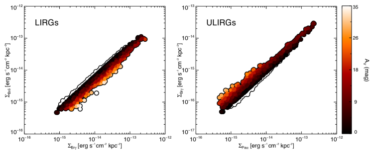
Fig. 3: Surface brightness distributions of the individual spaxels of LIRGs and ULIRGs. For clarity, we only plot a random distribution of the 20% and 50% of the points for LIRGs and ULIRGs, respectively. The colour code indicates the A_V value of each spaxel, whereas the points with A_V$<0$ are outlined with a black contour line. The increase in the extinction towards low surface brightness values is mainly due to the high uncertainties of the flux measurements, in particular in ULIRGs, where the highest A_V values correspond to the spaxels with the lower Br$\gamma$ surface brightness.

The 2D extinction / dust structure was derived using the Br$\gamma$/Br$\delta$ and Pa$\alpha$/Br$\gamma$ line ratios for LIRGs and ULIRGs respectively. Although the Br$\delta$ line is detected in most of the ULIRGs, its S/N is not high enough to map the emission and, in most of the cases, it is not sufficient to perform an integrated analysis of the emission.

As mentioned before, the maps of the different lines were constructed by fitting a single Gaussian profile on a spaxel-by-spaxel basis (see Fig. 6 and 1j). Based on the emission maps, we obtained the extinction in magnitudes (A_V) following the procedure outlined in Bedregal et al. (2009). We compared the theoretical ratio between the two lines (Br$\gamma$/Br$\delta$$=1.52$ and Pa$\alpha$/Br$\gamma$$=12.07$ at T$=10,000$ K and n${}_{\rm e}=10^{4}\,cm^{-3}$, case B; Osterbrock 1989) with the measurements for each spaxel. The extinction in magnitudes could be expressed in the form

$$\rm A_{\rm\lambda_{1}}-A_{\rm\lambda_{2}}=-2.5\cdot\rm log\left[\cfrac{\left(F_{\rm\lambda_{1}}/F_{\rm\lambda_{2}}\right)_{\rm O}}{\left(F_{\rm\lambda_{1}}/F_{\rm\lambda_{2}}\right)_{\rm T}}\right],$$ (1)

where F${}_{\rm\lambda_{\rm i},O}$ and F${}_{\rm\lambda_{\rm i},T}$ are the observed and theoretical fluxes for a line centred at $\rm\lambda_{\rm i}$. We made use of the extinction law described in Calzetti et al. (2000) to express Equation 1 in terms of the visual extinction A_V (A${}_{\rm Br\gamma}=0.096$ A_V, A${}_{\rm Br\delta}=0.132$ A_V and A${}_{\rm Pa\alpha}=0.145$ A_V).

Since the individual values of A_V are sensitive to the S/N of the weakest line (Br$\delta$ and Br$\gamma$ for LIRGs and ULIRGs respectively), we have only considered those spaxels where the weakest line has been detected above an S/N threshold of four to obtain reliable A_V. This effect is very significative in the case of the Br$\gamma$/Br$\delta$ ratio since the Br$\delta$ line lies close to the blue limit of the SINFONI K-band. As discussed in Paper I, this wavelength region is strongly affected by noise due to the sky emission, and the atmospheric transmission also decreases. This translates into a more complex local continuum determination, making the line fitting more uncertain. An excess in the continuum level estimation would decrease the line flux and, therefore, increase the extinction (see expression above). Although the Pa$\alpha$ line also lies in this region of the spectra, this effect is not so relevant, given the strength of the line (more than $\times 10$ the Br$\gamma$ emission), and it is in the numerator of Equation 1.

The 1$\rm\sigma$ uncertainties of the individual A_V values vary typically from 10–20% in central regions with high S/N, up to 70–80% in external areas of low surface brightness ($\Sigma\lower 2.0pt\hbox{$\,\buildrel\scriptstyle<\over{\scriptstyle\sim}\,$}$10^-16 erg s^-1 cm^-2 kpc^-2), with a median value of 30-35%. Owing to the larger individual errors in the low surface brightness areas, we observed an artificial increase in the A_V measurements, especially in the ULIRGs. This systematic effect is observed in Fig. 3, where the highest extinction values are measured in those spaxels with the lower Br$\gamma$ surface brightness. The A_V uncertainties are obtained from the corresponding errors in the fluxes of the two lines, which as described in Paper I, are estimated using Monte Carlo simulations. The advantage of this kind of error estimation is that uncertainties are directly measured from the spectra, so they not only include the effect from photon noise but also take uncertainties due to an improper continuum determination or line fitting into account.

Table 2: Integrated properties and statistics of the A_V distributions

Object	AV,nuclear		AV,nuclear		A${}_{\rm V,R_{\rm eff}}$		AV,FoV		AV,median	AV,mean		AV (P5)	AV (P95)	Nspaxel
(1)	(2)		(3)		(5)		(6)		(7)	(8)		(9)	(10)	(11)
IRASF12115-4656	$\cdots$		$\cdots$		7.7 $\pm$	0.1	5.2 $\pm$	0.1	4.9	6.3 $\pm$	8.1	-3.65	21.5	1533
IC5179	10.4 $\pm$	0.4	$\cdots$		4.2 $\pm$	0.1‡	4.2 $\pm$	0.1	4.4	5.2 $\pm$	6.3	-3.00	17.3	2099
NGC2369	16.8 $\pm$	0.2	$\cdots$		17.3 $\pm$	0.1	15.0 $\pm$	0.1	15.5	13.5 $\pm$	6.6	3.75	26.0	603
NGC5135	2.8 $\pm$	0.2	$\cdots$		3.8 $\pm$	0.1	3.7 $\pm$	0.1	4.2	4.7 $\pm$	4.5	-1.72	11.7	1100
NGC3110	$\cdots$		$\cdots$		7.4 $\pm$	0.1‡	7.4 $\pm$	0.1	7.9	7.9 $\pm$	5.8	-3.02	16.6	400
NGC7130	12.3 $\pm$	0.3	$\cdots$		11.8 $\pm$	0.2	8.7 $\pm$	0.1	6.2	5.9 $\pm$	6.5	-2.45	18.6	687
ESO320-G030	$\cdots$		$\cdots$		7.8 $\pm$	0.1	7.0 $\pm$	0.1	7.8	8.0 $\pm$	7.1	-2.82	20.1	1383
IRASF17138-1017	15.2 $\pm$	0.4	$\cdots$		11.1 $\pm$	0.1	7.0 $\pm$	0.1	7.6	6.1 $\pm$	5.6	-0.91	17.2	806
IC4687	10.6 $\pm$	0.1	$\cdots$		3.9 $\pm$	0.1	3.7 $\pm$	0.1	4.2	4.5 $\pm$	5.1	-1.74	13.1	3401
NGC3256†	$\cdots$		12.2 $\pm$	0.2	5.0 $\pm$	0.1	4.1 $\pm$	0.1	5.0	6.6 $\pm$	6.1	-2.73	16.8	4522
IRAS23128-5919	8.7 $\pm$	0.3	6.7 $\pm$	0.2	7.1 $\pm$	0.1	6.8 $\pm$	0.1	6.2	7.0 $\pm$	4.7	-1.60	13.4	1182
IRAS21130-4446	4.3 $\pm$	0.4	3.2 $\pm$	0.2	4.7 $\pm$	0.3	4.4 $\pm$	0.1	5.4	5.0 $\pm$	5.9	-1.80	15.5	214
IRAS22491-1808	4.1 $\pm$	0.3	4.5 $\pm$	0.2	5.5 $\pm$	0.1	5.3 $\pm$	0.1	6.4	6.5 $\pm$	5.1	-1.79	16.0	299
IRAS06206-6315	7.5 $\pm$	0.3	11.3 $\pm$	0.4	7.6 $\pm$	0.2	8.5 $\pm$	0.2	10.7	9.5 $\pm$	7.7	-3.05	22.7	114
IRAS12112+0305	8.9 $\pm$	0.3	8.4 $\pm$	0.2	9.2 $\pm$	0.2	8.5 $\pm$	0.1	8.2	9.0 $\pm$	6.2	-0.52	20.9	466
IRAS14348-1447	5.5 $\pm$	0.2	8.1 $\pm$	0.3	6.2 $\pm$	0.2	7.1 $\pm$	0.1	8.6	7.9 $\pm$	6.9	-1.04	20.6	301
IRAS17208-0014	8.0 $\pm$	0.2	$\cdots$		6.8 $\pm$	0.1	5.8 $\pm$	0.1	4.8	6.3 $\pm$	4.0	-1.61	10.8	485

5 Results and discussion

5.1 Two-dimensional extinction structure in LIRGs and ULIRGs

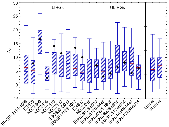
Fig. 4: Individual A_V distributions, on a spaxel-by-spaxel basis, of the galaxies of the sample ordered by increasing L_IR. The extremes of the distributions are the 5th and 95th percentiles (P₅ and P₉₅). The boxes illustrate the interquartile range, whereas the horizontal blue and red lines correspond to the median and the weighted mean of the distribution, respectively. The measurements of the nuclear extinction are plotted as black diamonds. The total A_V distributions for LIRGs and ULIRGs are shown on the right-hand side of the plot.

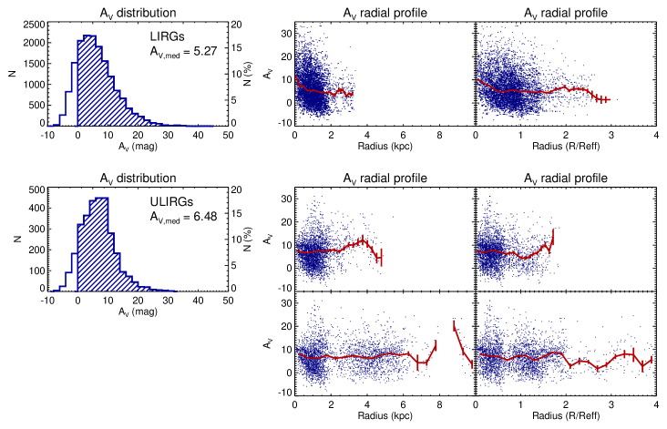
Fig. 5: A_V distributions and radial profiles of the LIRGs (top) and ULIRGs (bottom) subsamples on a spaxel-by-spaxel basis. The median A_V values of each distribution are shown in the left panels. In the central and right panels, the radial profiles are plotted in terms of the radius in kpc (centre) and in units of the H$\alpha$ effective radius (R_eff, right panel) extracted from Arribas et al. (2012). The red line represents the weighted mean of A_V and its error for different radial bins in steps of 1/30 of the total radial coverage. For the ULIRG subsample, we plotted the radial profile of the sample by considering each component of the systems separately (top) and the profile extracted by taking the brightest nucleus in the K-band continuum as the centre of the systems (bottom).

Our 2D extinction maps cover areas from $\sim$2 kpc to $\sim$12 kpc for LIRGs and ULIRGs, respectively (see Figs. 6 and 1j). The seeing-limited observations provide a linear resolution equivalent to a physical scale resolution of $\sim$0.2 kpc and $\sim$0.9 kpc for each subsample. On these scales, the extinction maps show that dust is not uniformly distributed, revealing a clumpy structure with almost transparent areas (A_V$\,\buildrel\scriptstyle<\over{\scriptstyle\sim}\,$1 mag) and regions where the visual extinction is higher than ten magnitudes.

In LIRGs, the extinction maps show a very irregular and clumpy structure on scales of $\sim$200-300 pc, already observed from near-IR continuum maps (Scoville et al. 2000). The higher A_V values are usually associated with the nuclear regions of the objects, although obscured extranuclear regions are also common. The star-forming regions with high Br$\gamma$ surface brightness, found along the dynamical structures like arms of rings, are typically low-extinction regions.

As shown in the radial profiles of NGC 3110 or IRASF 12115-4656 (Figs. 1b and 1e), the extinction increases inwards up to A_V$\sim$15–25 mag. This behaviour is also observed in ESO 320-G030 (Fig. 1d), where the emission is concentrated on a star-forming ring of $\sim$500–600 pc radius. Although the nucleus might also be obscured, the radial profile of this object is not as steep as in NGC 3110 or IRASF 12115-4656 and indicates that the lack of emission could also be due to the intrinsic distribution of the star-forming regions around the ring.

The morphology of the A_V maps in the ULIRG subsample suggest a patchy, non-uniform distribution of the dust, typically on physical scales of $\,\buildrel\scriptstyle>\over{\scriptstyle\sim}\,$1 kpc that correspond to our resolution limit. Owing to the higher linear resolution (i.e. kpc/spaxel) of the ULIRG subsample, the comparison with the LIRGs is not straightforward. As shown in Fig. 5, although our data samples similar areas of $\sim$1-2 R_eff, the dust structure is probed with significantly different spatial resolutions, owing to the factor $\times$5 in distance between both subsamples. This difference precludes our from resolving sub-kiloparsec structures in ULIRGs, such as the ones observed in the LIRG A_V maps, limiting our physical resolution to $\sim$1 kpc. As discussed in Sec. 5.4, these differences in the linear resolution between both subsamples not only shape the observed dust morphology in the more distant galaxies, but also might determine global measurements of the extinction, such as the median of the A_V distributions. In Sec. 5.5 we discuss how this distance effect would have direct implications for the study of high-z galaxies.

5.2 A_V distributions and radial profiles

Figures 6 and 1j show the A_V distributions for each galaxy. Although it is clear that most of the spaxels with A_V$<$0 have no physical meaning individually, we have kept them in the distributions since they do have statistical relevance. If we remove them from the distributions, we introduce a bias toward the high A_V values, displacing the mean and median of the distributions artificially. On the other hand, due to the S/N threshold adopted, we assure that most of those spaxels with A_V$<$0 are compatible with A_V$\sim$0 within the uncertainties.

The histograms show a wide variety of distributions, from narrow, peaked distributions, such as NGC 5135 or IC 4687 (Fig. 1f and 1h), concentrated towards low A_V values, to wide distributions such as NGC 3110 or IRAS 14348-1447 (Figs. 1b and 2c) that extend up to $\sim$30-35 mag. The median and weighted mean A_V values, together with the 5th and 95th percentiles of the distributions, are listed in Table 2. Figure 4 also compares the individual distributions of each galaxy of the sample, ordered by increasing L_IR. As shown in the figure, most of the individual values, within the interquartile ranges, are concentrated between A_V$\sim$1 and A_V$\sim$20 mag, and there is no clear evidence of any dependence with L_IR.

In LIRGs, the visual extinction ranges between A_V$\sim 1-20$ mag, whereas in ULIRGs, the A_V values range between A_V$\sim 2-15$ mag. In LIRGs, these values of the visual extinction are very similar although slightly lower than previous results in the mid-infrared from Spitzer, A_V$\lower 2.0pt\hbox{$\,\buildrel\scriptstyle<\over{\scriptstyle\sim}\,$}1-30$ mag with a mean value of $\sim$11 mag (Pereira-Santaella et al. 2010, Alonso-Herrero et al. 2012). On the other hand, ULIRGs show slightly higher values than previous measurements in the optical, from A_V$\,\buildrel\scriptstyle<\over{\scriptstyle\sim}\,$0.2 mag to $\sim 9$ mag (García-Marín et al. 2009), and significantly lower than mid-infrared measurements based on the silicate absorption feature at 9.7 $\mu$m, from A_V$\sim$6 mag up to A_V$\,\buildrel\scriptstyle>\over{\scriptstyle\sim}\,$40 mag (Imanishi et al. 2007).

These A_V values have to be considered as lower limits of the dust extinction, since the theoretical values of the ratios are based on the assumption that the gas is optically thin. However, it is well known that the central regions of these objects are dusty environments and that the observed recombination lines might have been originated at different depths within the star-forming regions. That also means that we would infer different extinction values from different emission line ratios, since the lines are probing different optical depths.

To compare the A_V distributions of LIRGs and ULIRGs, we combined all the available spaxels of each luminosity bin to obtain a typical A_V distribution. These distributions are shown in Fig. 4 and, in more detail, in Fig. 5. The median values of A_V for each subsample are similar, A_V${}_{\rm med}=5.3$ mag and A_V${}_{\rm med}=6.5$ mag, and the number of individual spaxels is $\sim$16000 for the LIRG distribution and $\sim$3000 for the ULIRG one. The shape of the distributions are, however, slightly different. Whereas the LIRG distribution seems to have more than 50% of the points concentrated within the range A_V$\simeq 1-10$ mag, the ULIRGs extend over a somewhat narrower range of A_V$\simeq 3-10$ mag and tend to reach higher A_V values on individual spaxels. On the other hand, the modes of the distributions are also different; whereas the LIRG distribution peaks at $\sim 3-4$ mag, the mode of the ULIRG distribution reaches up to $\sim 7-8$ mag. Although some of these differences might be intrinsic, we discuss in Section 5.4 that the physical sampling of the maps plays an important role in the study of the extinction, owing to the patchy structure of the dust.

We obtained the radial profiles of the extinction for every individual object of the sample and characteristic profiles for both LIRG and ULIRG subsamples. For this purpose, we adopted the same criterion as in Paper I to identify the central spaxel of each object with the brightest spaxel of the FoV in the K-band image (see Figs.6 and 1j). The only exception in NGC 3256, since the nucleus of this galaxy was not observed in the K-band (see Paper I for further details). For this object, we used the H-band continuum image of the nucleus to identify the central spaxel. For those systems with multiple nuclei (i.e. all the ULIRGs with the exception of IRAS 17208-0014), we also extracted the radial profiles of each component separately.

As shown in Figs. 6 and 1j, the profiles typically sample the inner $\sim 2$ kpc for the LIRGs and $\,\buildrel\scriptstyle<\over{\scriptstyle\sim}\,$6 kpc for the ULIRGs, and most of them have an almost flat or negative slope. LIRGs show steeper negative slopes than ULIRGs, especially in the central 0.5–1 kpc. In LIRGs, these slopes are typically of $\sim-$2.4 mag kpc^-1 on average, versus $\sim-$0.3 mag kpc^-1 in ULIRGs. This could be explained by the different sampling scales of both subsamples, since we cannot resolve the innermost regions of the ULIRGs with the resolution achieved for the LIRG subset. In those pre-coalescent systems with multiple nuclei, we found no systematic differences between the radial profiles of both components. These profiles typically sample the innermost $\sim 2-3$ kpc of each component of the system, and show no clear radial dependence of the extinction on these scales.

We extracted the radial profiles of the total A_V distributions of LIRGs and ULIRGs separately. Since each object has been observed with different sampling and physical scales, we also obtained the profiles in units of the effective radius R_eff, using the values from Arribas et al. (2012) obtained from H$\alpha$ maps. As shown in Fig. 5, the LIRG profile is almost flat beyond r$\sim$1 kpc or $\sim$0.5 R_eff, with an average value of A_V$\sim$5.3  mag. Within the central kiloparsec, the extinction increases up to $\sim$10 mag. The ULIRG subsample shows a very uniform profile, with a median value of A_V$\sim$6.0 mag and only local deviations due to the presence of double nuclei in some of the systems, or due to strong complexes of star formation at distances beyond 2-3 kpc radius (see Fig.2a and 2b for some examples). The radial profile shows small differences when extracted for each component separately, with an almost flat slope over the inner 2-3 kpc radius ($\sim$R_eff). The measurements beyond $r\sim$6 kpc or $r\sim$2 R_eff are very uncertain, owing to the lack of available spaxels and to the low surface brightness of the Br$\gamma$ emission in these regions. As mentioned before, the extinction in ULIRGs derived using Eq. 1 is highly affected by noise fluctuations of the Br$\gamma$ line.

5.3 Nuclear and integrated A_V measurements

We obtained integrated A_V measurements for different regions of interest in each object (Table 2). The uncertainties of the parameters are obtained by a Monte Carlo method of $\rm N=1000$ simulations, and do not take the 1$\sigma$ uncertainties of $\sim$5% into account in the absolute flux calibration (see Piqueras López et al. 2012). We found that, in $\sim$70% of the objects, its nucleus corresponds to a peak in the extinction, ranging from A_V$\sim$3 mag up to A_V$\sim$17 mag. These values of the nuclear extinction are higher than each median and mean A_V values in $\sim 57$% of the objects. However, there are some galaxies, such as NGC 3110 or IC 4687 (Figs. 1b and 1h), where the nucleus is completely obscured, and no measurements of the extinction are available. That the nucleus of the objects coincides with a peak of the extinction agrees with other studies in LIRGs and ULIRGs (see Alonso-Herrero et al. 2006 and García-Marín et al. 2009) based on H$\alpha$/H$\beta$ and Pa$\alpha$/Br$\gamma$ ratios, and with mid-infrared studies with Spitzer, based on the silicate absorption feature at 9.7 $\mu$m (Imanishi et al. 2007, Pereira-Santaella et al. 2010). These authors found that either the highest extinctions coincide with the nucleus of the objects or the nuclear regions are local maxima in the A_V maps.

For those objects with a double nucleus, we also presented integrated measurements of the extinction for the secondary one. Although almost all of the interacting systems in our sample are ULIRGs, NGC 3256 presents a well known, highly obscured nucleus $\sim 5$ arcsec to the south of the main one. Our measurements of the extinction of the southern nucleus of this object shows that it is one of the most extinguished regions in our sample, with A_V$\simeq$12.2 mag, in good agreement with previous works (Kotilainen et al. 1996, Alonso-Herrero et al. 2006, Díaz-Santos et al. 2008, Rich et al. 2011).

5.4 Dust clumpiness and the effect of the linear resolution.

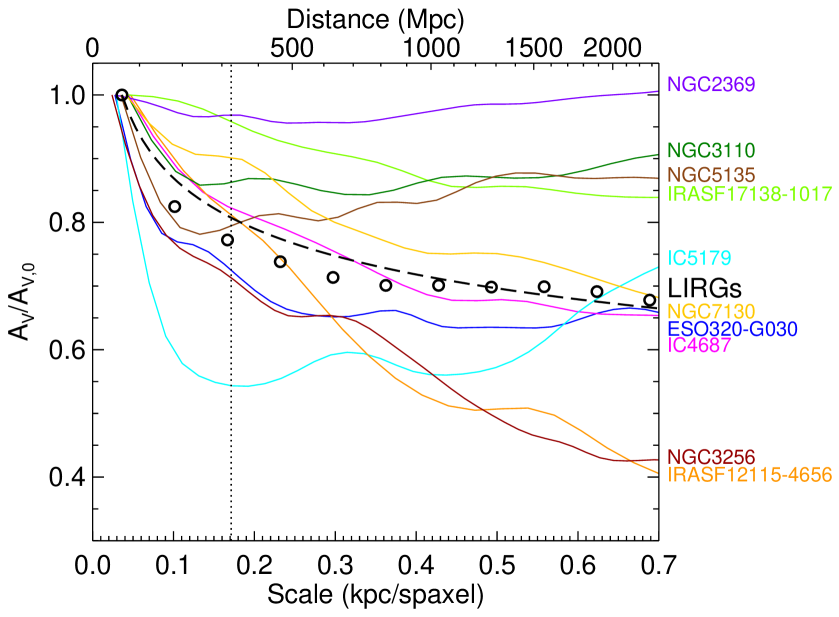
Fig. 6: Evolution of the computed median A_V of the individual distributions of the LIRG subsample as a function of scale/distance. The A_V values are normalised to the rest-framed distribution. The value that corresponds to the A_V distribution of the whole LIRG subsample is plotted as black circles and a power-law fit to the data as a dashed black line. The mean distance of the ULIRG subsample (328 Mpc) is plotted as a vertical dotted line for reference.

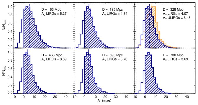
Fig. 7: Different simulations of the LIRGs A_V distribution for increasing distance (from top to bottom and left to right). The median of each distribution is highlighted with a vertical dashed line. The distance and the median A_V of the simulated distribution is annotated in each panel. The top left panel corresponds to the average distance of the ULIRG subsample, and shows the observed A_V distribution of the ULIRGs and its median, in yellow.

As mentioned in Section 5.1, the A_V maps reveal a patchy, clumpy structure of the dust at sub-kiloparsec and kiloparsec scales in LIRGs and ULIRGs, respectively. Given this non-uniform distribution, the measurements of the extinction at different distances might be affected by the physical scale of the observations. To probe how the pixel scale might bias the A_V measurements, we have obtained the A_V distribution of our LIRG sample simulating different scales, hence different distances. This distance effect because of the linear resolution might be even more relevant for high-z objects, where the structure is sampled on even larger scales of $\sim$1-2 kpc.

To simulate the distribution at further distances, we degraded the individual Br$\gamma$ and Br$\delta$ maps to different scales, and obtained maps of poorer spatial resolution. In this process, we only considered the same valid spaxels as in the original maps. Once the maps were degraded, we obtained the A_V distributions of each individual object as described in Section 4, which were finally combined in one single distribution.

Since the FoV of our SINFONI observation is limited to $\sim 8"\times 8"$, we could only sample the innermost $\sim 3\times 3$ kpc of the LIRGs (typically $\sim$R_eff). If we translate these scales to a distance that is ten times larger, these $\sim 3$ kpc are equivalent to an angular distance of $\sim$1”, i.e. 1/8 of the FoV or $\sim 8$  spaxels. The lack of data from the external regions of the local objects keeps the extrapolation to larger distances from beeing straight-forward.

Figure 6 shows the relation of the median of the individual A_V simulated distributions to the sampling scale/distance, for each galaxy in the LIRG subsample. Although each curve shows a different behaviour that depends on the particular gas and dust distribution, there is a general trend towards lower A_V values as distance increases. This decrement of the median value of the visual extinction is also observed when we consider the distribution of LIRGs as a class, adding all the individual spaxels of the LIRG subsample in a single distribution, as shown in the figure. To parametrize this observed decrement of the median A_V of the LIRG distribution with the sampling scale/distance, we fitted the data points to a simple power-law model, and found that the best-fit model corresponds to

$$\rm A_{\rm V}/A_{\rm V0}\simeq\rm(D/D_{\rm 0})^{-0.13}\simeq\rm(S/S_{\rm 0})^{-0.14},$$ (2)

where A_V and S are the median values of the A_V distribution and the physical scale at a distance D, respectively, and A${}_{\rm V0}=5.27$ mag and S${}_{\rm 0}=290$ pc arcsec^-1 are the median values of the rest-frame A_V distribution and median physical scale at the mean distance of the LIRGs subset, D${}_{\rm 0}=63.3$ Mpc, respectively.

In figure 7, we show in detail the observed A_V distribution of the LIRG subsample and the simulated distributions for increasing distances. The different panels reveal that not only the median value of the distribution decreases when the galaxies are sampled on a larger physical scale, but also that the shape of the distribution is slightly different, becoming narrower than the rest-framed distribution, and more compact. The mode of the simulated distribution also changes with respect to the ULIRG observed distribution, and becomes lower than the median. As shown in Fig. 6, the difference between the rest-frame extinction, A_V0, and the simulated A_V increases rapidly within the first D$\sim$700 Mpc, and seems to reach an asymptotic value of A_V/A${}_{\rm V0}\sim$0.65 beyond that distance.

The non-uniform distribution of the dust, even on small scales, makes that, at a given resolution unit, we map both obscured regions and areas where the interstellar medium is more transparent. This average is biased towards the brightest regions, which are those were the emission is less absorbed. The result is that, on average, the dust distribution is smoothed, becomes narrower, and the A_V values that we measure are biased towards the lowest values.

As mentioned in Section 5.2, we measured a median extinction of A_V${}_{\rm,LIRGs}=5.3$ and A_V${}_{\rm,ULIRGs}=6.5$ magnitudes for our LIRG and ULIRG subsamples, respectively. Since the average distance of each subsample is $\sim 63$ Mpc and $\sim 328$ Mpc (see Paper I), this factor $\sim$5 in distance and sampling scale (from $\sim$0.2 kpc to $\sim$0.9 kpc on average, respectively) translates to a decrease in the measured A_V of $\sim$1.2 mag, as shown in Fig. 7 (top right panel). If we assume that LIRGs and ULIRGs have similar structures and apply the same correction to the ULIRGs subsample, we find that the average A_V in the ULIRGs, corrected from distance effects, reaches A_V$\sim$8.0 mag, i.e. $\sim$2.8 mag higher than in LIRGs.

Besides this resolution/distance effect, the difference between the observed A_V distribution in LIRGs and ULIRGs could also be interpreted in terms of intrinsic differences in the morphology between both classes. Although there seems to be a general trend for LIRGs as a class that suggest that the observed A_V decreases with the distance/resolution, Fig.6 also shows that the behaviour of each individual galaxy is very different, and depends strongly on the particular morphology of the dust distribution. These differences among the objects of the LIRGs subset suggest that the correction to the observed A_V could not be accurate for individual galaxies, and would only reflect a general trend for LIRGs as a class.

5.5 Implication for extinction-corrected properties in high-z galaxies

There are different observational proofs that suggest that sub-millimetre galaxies (SMGs) could be the high-z analogous of local (U)LIRG. The sub-millimetre and radio fluxes of this population of galaxies indicate that their bolometric luminosities are comparable to local ULIRGs, whereas their mid-IR emission seems to be similar to the observed in local LIRGs (Kovács et al. 2006, Takata et al. 2006, Menéndez-Delmestre et al. 2009). Besides this, recent IFS-based observations of SMGs reveal that they present evidence of clumpy star formation on kiloparsec scales and similar star-formation rate surface densities ($\Sigma_{\rm SFR}$) to the local counterparts (Nesvadba et al. 2007, Harrison et al. 2012, Alaghband-Zadeh et al. 2012, Menéndez-Delmestre et al. 2013). It is well known that these high-z galaxies may be highly obscured and that a combination of intense dust-obscured star formation and dust-enshrouded AGN activity would be responsible for the high infrared luminosities of these objects (Blain et al. 2002). HST-NICMOS and ACS observations reflect structured dust obscuration in these objects (Swinbank et al. 2010). In particular, Takata et al. (2006) find that the internal extinction in these objects are similar to the extinction in local ULIRGs, and measured a median extinction of A_V$=2.9\pm 0.5$ mag in a sample of SMGs at z$\sim$1.0–3.5 using the H_α/H_β flux ratio.

Clumpy and dusty star-forming structures have also been identified at high redshifts in more common star forming galaxies (i.e. the so called Main Sequence star forming galaxies). These galaxies have (sub)kpc star-forming clumps mostly spread over galactocentric distances of few to several kpc (Förster Schreiber et al. 2011a, 2011b, Genzel et al. 2011), and with internal nebular extinctions of 2 to 4 magnitudes, assuming $\rm A_{v,H_{\alpha}}=A_{v,stellar}/0.44$ (Förster Schreiber et al. 2009, Wuyts et al. 2011).

In the previous subsection we showed that the distance/linear scale may play an important role in deriving the internal extinction properties of LIRGs and ULIRGs, by comparing both populations of galaxies locally, albeit with a difference of a factor $\times$5 in distance between both subsamples. According to the simulations, the median extinction measured in a given galaxy decreases when placed at increasing distances. This effect is due to the fixed angular resolution of the IFS data that translates into a larger physical scale per spatial resolution element (spaxel) as the distance to the galaxy increases, and is particularly important when the physical scales sampled by the spaxel are much larger than that of the intrinsic clumpy structure of the dust distribution and star-forming regions.

It is clear that if the intrinsic star-forming structure of high-z galaxies is in general similar to that of our local LIRGs (i.e. mostly disks) and ULIRGs (i.e. mostly interacting), the smearing effect mentioned above would have a direct impact in the derivation of their 2D internal extinction values, and of all relevant subsequent extinction corrected properties such as star formation surface densities, KS-laws, and overall star formation rates. This would certainly be the case not only with seeing-limited near-IR IFS, heavily undersampling the galaxies at redshifts of 1 to 3, with each spaxel corresponding to about 1.5-2 kpc, but even when using AO assisted IFS where the spaxel (50 to 100 mas) translates to about 0.4 to 0.8 kpc. Thus, if the results given by Eq. 2 (see also Fig. 6) are applied to high-z galaxies, the extinction values derived directly from the observed optical emission line ratios would require to be increased by a factor 1.4 on average. This correction would correspond to an additional increase in the H_α flux by a factor $\sim$3 and hence, in the extinction-corrected SFR and $\Sigma_{\rm SFR}$.

Finally, it is worth noticing that this distance effect could also have a minor wavelength dependency. The method presented here to derive the A_V values is based on specific emission line ratios in the near-infrared. Since these lines originate in regions of higher optical depths than the optical emission lines, and the stellar continuum measured at optical wavelengths, differences in the amount and/or distance dependency could appear. It would be worth exploring these effects with a suitable set of data, in particular if, as in many high-z studies, the A_V corrections applied to the observed H$\alpha$ flux is obtained indirectly using the standard Calzetti recipe A_Hα = 7.4 E(B–V), where E(B–V)_gas = 0.44 E(B–V)_stars (Calzetti et al. 2000, 2001)

6 Summary

In this paper, we presented a detailed 2D study of the extinction structure of a representative local sample of 10 LIRGs and 7 ULIRGs, based on VLT-SINFONI IFS K-band observations. We sample the central $\sim 3\times 3$ kpc for LIRGs and the $\sim 12\times 12$ kpc for ULIRGs, with average linear resolutions (FWHM) of $\sim$0.2 kpc and $\sim$0.9 kpc, respectively. The extinction maps are based on measurements of the Br$\gamma$/Br$\delta$ line ratio for LIRGs and of the Pa$\alpha$/Br$\gamma$ line ratio for ULIRGs.

In agreement with previous studies, we found that the distribution of the dust in these galaxies presents a patchy structure on sub-kiloparsec scales, with regions almost transparent with A_V$\sim$0 to heavily obscured areas with A_V values up to $\sim 20-30$ mag. In most of the objects in the sample ($\sim$70%), the nucleus of the galaxy coincides with the peak in the extinction maps, with values that range from A_V$\sim 3$ mag up to A_V$\sim$17 mag.

We obtained the A_V distribution of the individual galaxies on a spaxel-by-spaxel basis (see Fig. 4). The individual A_V distributions show a wide range of values with most of them spread between A_V$\sim$1 and A_V$\sim$20 mag, with no clear evidence of any dependence with L_IR. However, as a class (see Fig. 5), ULIRGs show A_V values (median of 6.5 mag, mode of $\sim$7-8 mag) higher than those for LIRGs (median of 5.3 mag, mode of $\sim$3-4 mag). The A_V distribution in LIRGs shows a mild decrease as a function of galactocentric distances of up to 1 kpc and a flattening at larger distances (2-3 kpc). No similar behaviour is detected in ULIRGs, most likely owing to the lower linear resolution of the observations.

To study the effect of the spatial sampling (i.e. physical scale per spaxel) in the derived extinction values at increasing galaxy distances, the individual Br$\gamma$ and Br$\delta$ maps of our subsample of local LIRGs (at an average distance of 63 Mpc) have been artificially smeared. These simulations have shown that the spatial resolution plays an important role in shaping the A_V distributions. The median value of the visual extinction measured on the LIRG subsample decreases as a function of the linear resolution/distance by a factor $\sim$ 0.8 at the average distance (328 Mpc, 0.2 kpc/spaxel) of our ULIRG sample, and up to $\sim$0.67 for distances above 800 Mpc (0.4 kpc/spaxel). This distance effect would have implications in the derivation of the intrinsic extinction, and subsequent properties, such as SFR, $\Sigma_{\rm SFR}$, and the KS-law, in high-z star-forming galaxies, even in AO-based spectroscopy. If local LIRGs are analogues of the main-sequence star-forming galaxies at cosmological distances, the extinction values (A_V) derived from the observed emission lines in these high-z sources would need to be increased by a factor 1.4 on average.

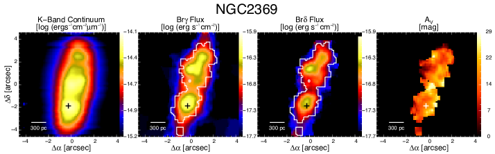
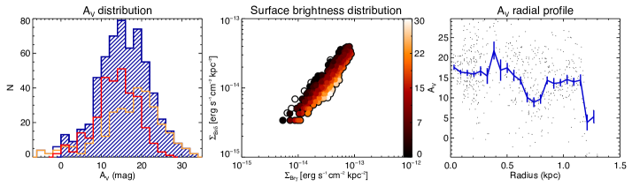
Fig. 1a: NGC 2369. Top panels show the SINFONI K band continuum emission, the observed maps (not corrected from extinction) of the lines Br$\gamma$ at 2.166 ${\mu}$m and Br$\delta$ at 1.945 ${\mu}$m, together with the A_V map. The white contour englobes those spaxels above $\rm S/N=4$ considered to build the A_V map and distribution. The brightest spaxel of the K band continuum is marked with a plus symbol (+), and has been used as reference to obtain the radial profile in the bottom right panel. The secondary nucleus, if present, is marked with a cross ($\times$). Bottom left panel shows the the Av distribution of all valid spaxels (blue histogram) and the distributions of the those spaxels above (red) and below (yellow) the median value of the Br$\delta$ S/N distribution. The relationship between the surface brightness of the lines and the A_V is shown in the central panel, where the points with A_V$<$0 are outlined with a black contour. Finally, the radial distribution of the extinction is shown in the bottom right panel, where the blue line represents the mean value of A_V for different radial bins and its error. The bins are obtained as the 1/30 of the total radial coverage of the map.

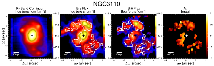
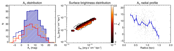
Fig. 1b: NGC 3110. Same as Fig. 1a but for NGC 3110

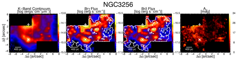
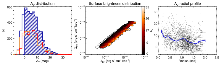
Fig. 1c: NGC 3256. Same as Fig. 1a but for NGC 3256. Please note that the central spaxel lays outside the FoV since the nucleus was not observed in K-band. See text and Paper I for further details.

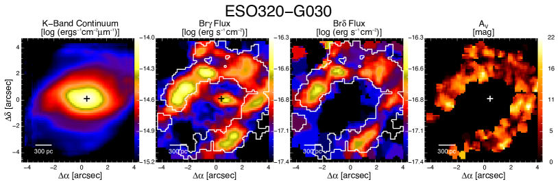
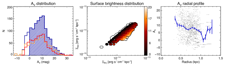
Fig. 1d: ESO 320-G030. Same as Fig. 1a but for ESO 320-G030

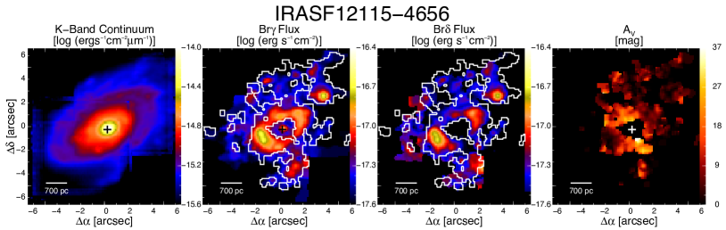
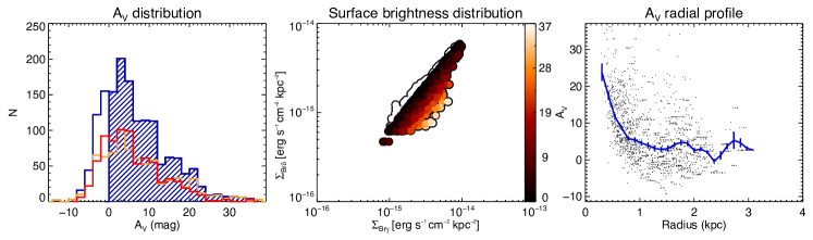
Fig. 1e: IRASF 12115-4656. Same as Fig. 1a but for IRASF 12115-4656

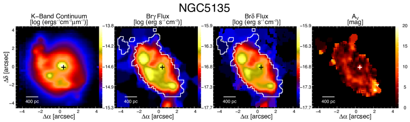
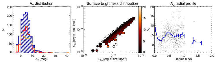
Fig. 1f: NGC 5135. Same as Fig. 1a but for NGC 5135

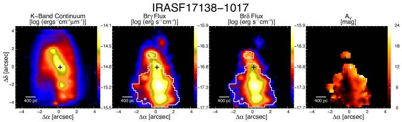
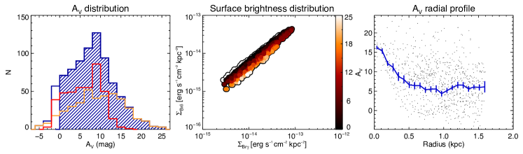
Fig. 1g: IRASF 17138-1017. Same as Fig. 1a but for IRASF 17138-1017

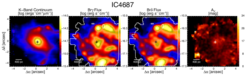
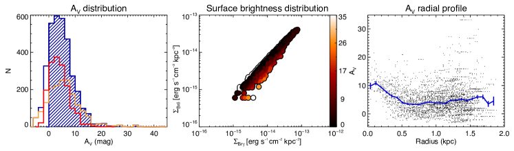
Fig. 1h: IC 4687. Same as Fig. 1a but for IC 4687

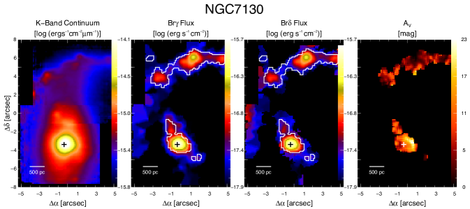
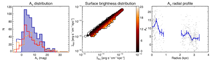
Fig. 1i: NGC 7130. Same as Fig. 1a but for NGC 7130

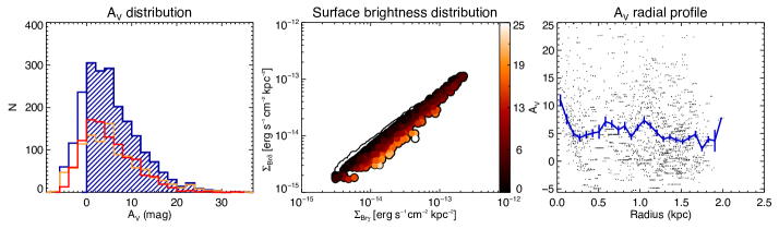
Fig. 1j: IC 5179. Same as Fig. 1a but for IC 5179

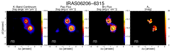
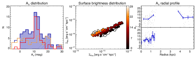
Fig. 2a: IRAS 06206-6315. Top panels show the SINFONI K band continuum emission, the observed maps (not corrected from extinction) of the lines Pa$\alpha$ at 1.876 ${\mu}$m and Br$\gamma$ at 2.166 ${\mu}$m, together with the A_V map. The white contour englobes those spaxels above $\rm S/N=4$ considered to build the A_V map and distribution. The brightest spaxel of the K band continuum is marked with a plus symbol (+), and has been used as reference to obtain the radial profile in the bottom right panel. The secondary nucleus, if present, is marked with a cross ($\times$). Bottom left panel shows the Av distribution of all valid spaxels (blue histogram) and the distributions of the those spaxels above (red) and below (yellow) the median value of the Br$\gamma$ S/N distribution. The relationship between the surface brightness of the lines and the A_V is shown in the central panel, where the points with A_V$<$0 are outlined with a black contour. Finally, the radial distribution of the extinction is shown in the bottom right panel, where the blue line represents the mean value of A_V for different radial bins and its error. The bins are obtained as the 1/30 of the total radial coverage of the map. For those objects with multiple components, the top inset shows the A_V radial profile of the system taking the main nucleus as the centre, whereas the bottom subpanel shows the radial profile obtained by extracting the profiles of each component separately and plotting them in the same reference frame.

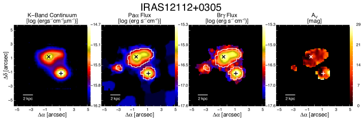
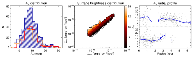
Fig. 2b: IRAS 12112+0305. Same as Fig. 2a but for IRAS 12112+0305.

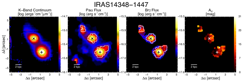
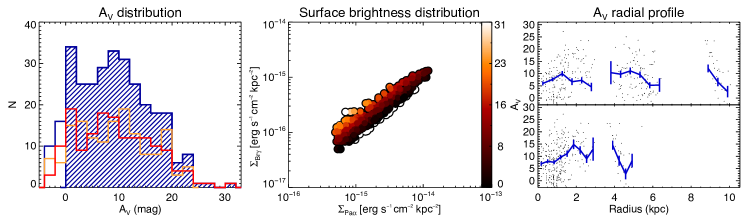
Fig. 2c: IRAS 14348-1447. Same as Fig. 2a but for IRAS 14348-1447.

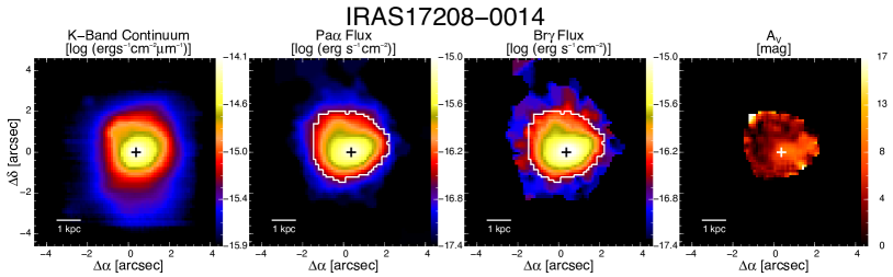
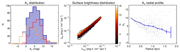
Fig. 2d: IRAS 17208-0014. Same as Fig. 2a but for IRAS 17208-0014.

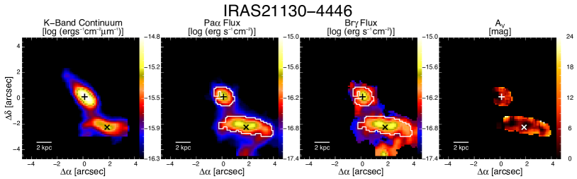
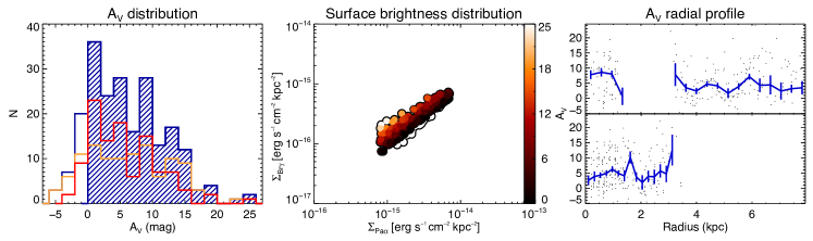
Fig. 2e: IRAS 21130-4446. Same as Fig. 2a but for IRAS 21130-4446.

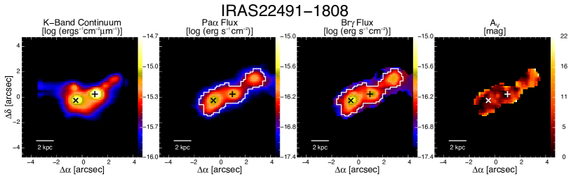
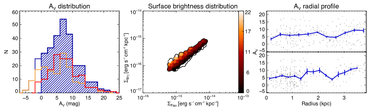
Fig. 2f: IRAS 22491-1808. Same as Fig. 2a but for IRAS 22491-1808.

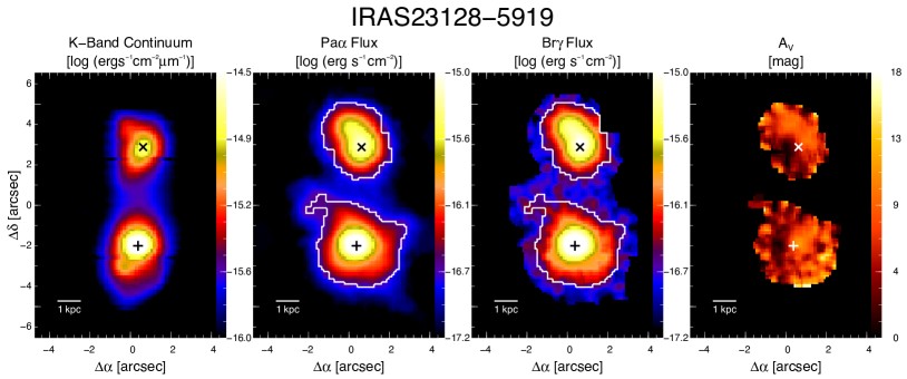
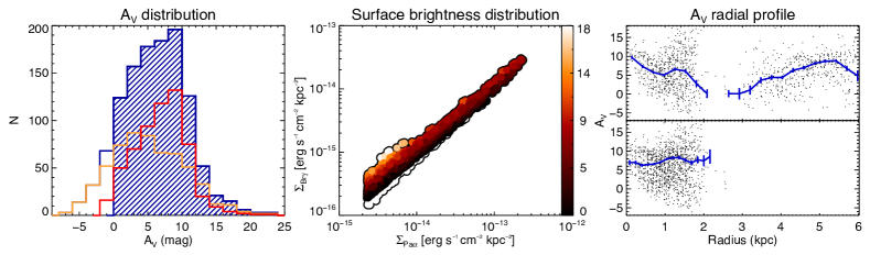
Fig. 2g: IRAS 23128-5919. Same as Fig. 2a but for IRAS 23128-5919.

References

- Alaghband-Zadeh et al. (2012) Alaghband-Zadeh, S., Chapman, S. C., Swinbank, A. M., et al. 2012, MNRAS, 424, 2232
- Alonso-Herrero et al. (2012) Alonso-Herrero, A., Pereira-Santaella, M., Rieke, G. H., & Rigopoulou, D. 2012, ApJ, 744, 2
- Alonso-Herrero et al. (2006) Alonso-Herrero, A., Rieke, G. H., Rieke, M. J., et al. 2006, ApJ, 650, 835
- Arribas et al. (1998) Arribas, S., Carter, D., Cavaller, L., et al. 1998, SPIE, 3355, 821
- Arribas et al. (2012) Arribas, S., Colina, L., Alonso-Herrero, A., et al. 2012, A&A, 541, A20
- Arribas et al. (2008) Arribas, S., Colina, L., Monreal-Ibero, A., et al. 2008, A&A, 479, 687
- Bedregal et al. (2009) Bedregal, A. G., Colina, L., Alonso-Herrero, A., & Arribas, S. 2009, ApJ, 698, 1852
- Blain et al. (2002) Blain, A. W., Smail, I., Ivison, R. J., Kneib, J. P., & Frayer, D. T. 2002, PhR, 369, 111
- Calzetti (2001) Calzetti, D. 2001, PASP, 113, 1449
- Calzetti et al. (2000) Calzetti, D., Armus, L., Bohlin, R. C., et al. 2000, ApJ, 533, 682
- Cappellari & Copin (2003) Cappellari, M. & Copin, Y. 2003, MNRAS, 342, 345
- Colina et al. (2000) Colina, L., Arribas, S., Borne, K. D., & Monreal, A. 2000, ApJ, 533, L9
- Díaz-Santos et al. (2008) Díaz-Santos, T., Alonso-Herrero, A., Colina, L., et al. 2008, ApJ, 685, 211
- Eisenhauer et al. (2003) Eisenhauer, F., Abuter, R., Bickert, K., et al. 2003, SPIE, 4841, 1548
- Förster Schreiber et al. (2009) Förster Schreiber, N. M., Genzel, R., Bouché, N., et al. 2009, ApJ, 706, 1364
- Förster Schreiber et al. (2011a) Förster Schreiber, N. M., Shapley, A. E., Erb, D. K., et al. 2011a, ApJ, 731, 65
- Förster Schreiber et al. (2011b) Förster Schreiber, N. M., Shapley, A. E., Genzel, R., et al. 2011b, ApJ, 739, 45
- García-Marín et al. (2009) García-Marín, M., Colina, L., & Arribas, S. 2009, A&A, 505, 1017
- García-Marín et al. (2006) García-Marín, M., Colina, L., Arribas, S., Alonso-Herrero, A., & Mediavilla, E. 2006, ApJ, 650, 850
- Genzel et al. (1998) Genzel, R., Lutz, D., Sturm, E., et al. 1998, ApJ, 498, 579
- Genzel et al. (2011) Genzel, R., Newman, S., Jones, T., et al. 2011, ApJ, 733, 101
- Goldader et al. (1995) Goldader, J. D., Joseph, R. D., Doyon, R., & Sanders, D. B. 1995, ApJ, 444, 97
- Harrison et al. (2012) Harrison, C. M., Alexander, D. M., Swinbank, A. M., et al. 2012, MNRAS, 426, 1073
- Imanishi et al. (2007) Imanishi, M., Dudley, C. C., Maiolino, R., et al. 2007, ApJS, 171, 72
- Kotilainen et al. (1996) Kotilainen, J. K., Moorwood, A. F. M., Ward, M. J., & Forbes, D. A. 1996, A&A, 305, 107
- Kovács et al. (2006) Kovács, A., Chapman, S. C., Dowell, C. D., et al. 2006, ApJ, 650, 592
- LeFèvre et al. (2003) LeFèvre, O., Saisse, M., Mancini, D., et al. 2003, SPIE, 4841, 1670
- Lonsdale et al. (2006) Lonsdale, C. J., Farrah, D., & Smith, H. E. 2006, Astrophysics Update 2, 285
- Markwardt (2009) Markwardt, C. B. 2009, Astronomical Data Analysis Software and Systems XVIII ASP Conference Series, 411, 251
- Menéndez-Delmestre et al. (2009) Menéndez-Delmestre, K., Blain, A. W., Smail, I., et al. 2009, ApJ, 699, 667
- Menéndez-Delmestre et al. (2013) Menéndez-Delmestre, K., Blain, A. W., Swinbank, M., et al. 2013, arXiv, astro-ph.CO
- Nardini et al. (2010) Nardini, E., Risaliti, G., Watabe, Y., Salvati, M., & Sani, E. 2010, MNRAS, 405, 2505
- Nesvadba et al. (2007) Nesvadba, N. P. H., Lehnert, M. D., Genzel, R., et al. 2007, ApJ, 657, 725
- Osterbrock (1989) Osterbrock, D. E. 1989, Astrophysics of Gaseous Nebulae and Active Galactic Nuclei. University Science Books, Mill Valley, USA
- Pereira-Santaella et al. (2010) Pereira-Santaella, M., Alonso-Herrero, A., Rieke, G. H., et al. 2010, ApJS, 188, 447
- Piqueras López et al. (2012) Piqueras López, J., Colina, L., Arribas, S., Alonso-Herrero, A., & Bedregal, A. G. 2012, A&A, 546, 64
- Rich et al. (2011) Rich, J. A., Kewley, L. J., & Dopita, M. A. 2011, ApJ, 734, 87
- Roth et al. (2005) Roth, M. M., Kelz, A., Fechner, T., et al. 2005, PASP, 117, 620
- Sanders et al. (2003) Sanders, D. B., Mazzarella, J. M., Kim, D.-C., Surace, J. A., & Soifer, B. T. 2003, AJ, 126, 1607
- Sanders & Mirabel (1996) Sanders, D. B. & Mirabel, I. F. 1996, ARA&A, 34, 749
- Scoville et al. (2000) Scoville, N. Z., Evans, A. S., Thompson, R., et al. 2000, AJ, 119, 991
- Soifer et al. (1984) Soifer, B. T., Neugebauer, G., Helou, G., et al. 1984, ApJ, 283, L1
- Swinbank et al. (2010) Swinbank, A. M., Smail, I., Chapman, S. C., et al. 2010, MNRAS, 405, 234
- Takata et al. (2006) Takata, T., Sekiguchi, K., Smail, I., et al. 2006, ApJ, 651, 713
- Veilleux et al. (2009) Veilleux, S., Kim, D.-C., Rupke, D. S. N., et al. 2009, A&A, 701, 587
- Wright (2006) Wright, E. L. 2006, PASP, 118, 1711
- Wuyts et al. (2011) Wuyts, S., Förster Schreiber, N. M., Lutz, D., et al. 2011, ApJ, 738, 106