2MTF II. New Parkes 21-cm observations of 303 southern galaxies

Abstract

We present new 21-cm neutral hydrogen (H i) observations of spiral galaxies for the 2MASS Tully Fisher (2MTF) survey. Using the 64-m Parkes radio telescope multibeam system we obtain 152 high signal-to-noise H i spectra from which we extract 148 high-accuracy ($<5\%$ error) velocity widths and derive reliable rotation velocities. The observed sample consists of 303 southern ($\delta<-40\degr$) galaxies selected from the 2MASS Redshift Survey (2MRS) with $K_{s}<11.25$ mag, $cz<10,000$ km s^-1 and axis ratio $b/a<0.5$. The H i observations reported in this paper will be combined with new H i spectra from the Green Bank and Arecibo telescopes, together producing the most uniform Tully-Fisher survey ever constructed (in terms of sky coverage). In particular, due to its near infrared selection, 2MTF will be significantly more complete at low Galactic latitude ($|b|<15^{\circ}$) and will provide a more reliable map of peculiar velocities in the local universe.

1 Introduction

In the local Universe, the galaxy distribution reveals large structures such as walls, filaments and voids on scales up to 100 Mpc (de Lapparent et al., 1986; Jones et al., 2009; Scrimgeour et al., 2012). The gravitational effects exerted on individual galaxies by this inhomogeneous distribution results in peculiar (non-Hubble) motions that can be used to probe the underlying mass distribution and constrain the cosmological models (Erdoğdu et al., 2006). Much of our understanding of the local Universe comes from optical sky surveys. However, infrared and 21-cm surveys are increasingly important because of lower dust extinction and their closer correspondence to stellar luminosity and total mass, respectively.

An important application obtained from the combination of galaxy photometry and H i spectra is the infrared Tully-Fisher relation, which is an empirical relation between the luminosity and rotational velocity of spiral galaxies (Tully & Fisher, 1977). The near-infrared Tully-Fisher relation has increased precision over optical formulations (Aaronson et al., 1982) and can be calibrated via primary distance indicators such as Cepheids or the Tip of the Red Giant Branch (Tully & Courtois, 2012), it can be used to measure redshift-independent distances of local spiral galaxies. With these redshift-independent distances, we can calculate the peculiar velocity field.

In the last few decades, a number of Tully-Fisher surveys have been conducted, including those described in Giovanelli et al. (1997); Springob et al. (2007); Tully et al. (2008). These are typically limited by source selection criteria and sky coverage. For instance, the SFI++ survey (Haynes et al., 1999a, b; Masters et al., 2006; Springob et al., 2007, and references therein), which is the largest Tully-Fisher survey to date, was selected optically in $I$-band and can only cover Galactic latitudes $|b|>15^{\circ}$. The part of the sky not covered by SFI++ is known as the Zone of Avoidance (ZoA) and is difficult to observe because of the effects of dust and stellar crowding in the plane of our Galaxy.

The 2MASS Tully-Fisher Survey (2MTF, Masters, 2008; Masters et al., 2008; Hong et al., 2013) gets around this by using infrared and 21-cm radio observations to improve our knowledge and model of the mass distribution of the local Universe. 2MTF is based on a source list selected from the 2 Micron All-Sky Survey Extended Source Catalog (2MASS XSC, Jarrett et al., 2000), and combines high-quality infrared photometry and 21-cm rotation widths for all bright inclined spirals in the 2MASS Redshift Survey (2MRS, Huchra et al., 2012). The final 2MTF sample is expected to contain about 3,000 high-quality H i widths, including new observed H i widths by our group using the Green Bank Telescope (GBT) and Parkes radio telescope, H i widths from the ALFALFA survey (Giovanelli et al., 2005; Haynes et al., 2011) and high quality archival H i widths.

In this paper, we present H i observations of 303 southern 2MTF galaxies using the Parkes radio telescope. We describe our observations and data reduction processes in Section 2. In Section 3, we discuss the statistical properties of the data. Some notable detections are presented in Section 4. We give the summary in the last section.

2 Observations and Data reduction

The 2MTF survey aims to measure distances for all bright inclined spirals in 2MRS. We selected galaxies from the 2MRS catalog that met the following criteria: total $K_{s}$ magnitudes $K_{s}<11.25$ mag, $cz<10,000$ km s^-1, and axis ratio $b/a<0.5$. In addition, we added some galaxies with $K_{s}<11.75$ mag in order to increase the number of H i detections at declinations south of $-40^{\circ}$. The target list contains $\sim 6,000$ 2MRS galaxies that meet our selection criteria. By 2006, when we made our observation plan, 40% of the target galaxies already had archival rotation width measurements for Tully-Fisher distances (mainly from Theureau et al., 1998; Springob et al., 2005; Theureau et al., 2005), but with very uneven sky coverage, especially in the southern hemisphere. To supplement these archival measurements, we observed $\sim 1,000$ galaxies with $\delta>-40^{\circ}$ with the Green Bank Telescope to peak flux limits $S_{p}\geq 10$ mJy (Masters et al., in prep). For $\delta<-40^{\circ}$ only about 25% of the 1018 selected 2MRS galaxies had high-quality H i width measurements already available. Of the remaining 754 galaxies, 303 were deemed not to be confused in the 15 arcmin beam of the Parkes telescope, and were observed.

The southern galaxies were observed in six semesters between 2006 and 2012 (see Table 1 for more details) using the 21-cm multibeam receiver (Staveley-Smith et al., 1996). The multibeam correlator was used with a bandwidth of 8 MHz, divided into 1024 channels, providing a channel spacing of $\sim 1.6$ km s^-1. During the observation of each galaxy, the band was centered on the 2MRS redshift of the target galaxy. The observations were done in beam switching mode (MX mode) using the 7 high-efficiency central beams of the receiver each with two orthogonal linear polarizations. In MX mode, the target galaxy was tracked in turn with each beam. When a beam was not pointing at the galaxy (off position), the data collected by this beam was used as a reference spectrum for calibration of the on-galaxy spectrum.

Table 1: Details of Parkes observations

Observing dates	Observing hours	Number of galaxies
2006 Nov 3 - Nov 12	80	68
2007 May 20 - Jun 3	160	84
2007 Nov 1 - Nov 7	55	22
2007 Dec 5 - Dec 14	65	32
2008 May 12 - May 22	146	115
2008 Sep 24 - Oct 1	72	34
2011 Oct 1 - Oct 6	40	33
2012 Mar 11 - Mar 16	40	28

Each galaxy was observed for a minimum of 35-min (i.e. each of the 7 beams was on-source for 5-min), with the correlator writing a spectrum every 5 seconds. After a preliminary data reduction, unless the observer estimated the signal-to-noise (S/N) of the galaxy H i spectrum to be $\ga$10, the process was repeated. We define S/N as the ratio of the peak H i flux per channel divided by the rms noise. Galaxies with profiles which were deemed too weak to reach that S/N ratio in a reasonable time were not observed further.

The data were bandpass and Doppler corrected using livedata (Barnes et al., 2001) with a MEDIAN estimator, all spectra were corrected to the solar system barycenter. Gridding was done by gridzilla, using a MEDIAN gridding algorithm. In order to obtain identical H i parameter measurements to the GBT observations (Masters et al., in prep.), we adopted the same GBTIDL routines. Using 3-channel Hanning smoothing we obtained a velocity resolution of 3.3 km s^-1and rms of 2 - 17 mJy.

The main source of radio frequency interference (RFI) was the L3 beacon of the Global Position System (GPS) satellite near 1381 MHz (equivalent to $cz\sim 8306$ km s^-1), which occurred approximately every 30-min. In order to avoid contaminating the H i spectra of galaxies with velocities near this RFI signal, we reduced their on-source integration time from 35 to 21-min.

Of the 303 observed galaxies: 152 have spectra whose S/N and spectrum profile are good enough for H i parameter measurements; 36 were poorly detected; and the remaining 115 galaxies were not detected. We report the raw and corrected H i parameters for the 152 well-detected galaxies in this paper. Figure 1 shows the sky distribution of all Parkes observed galaxies.

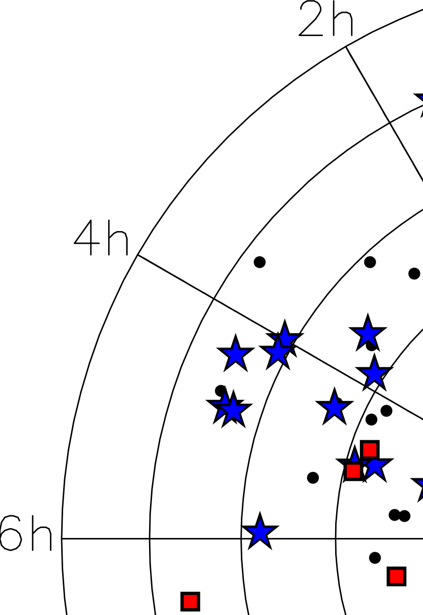
Figure 1: The distribution of Parkes observed galaxies. The blue stars indicate the 152 well-detected galaxies; poorly-detected galaxies are plotted with red squares; the black dots are the non-detected galaxies. The thick lines trace the galactic latitudes $b=5^{\circ}$ and $b=-5^{\circ}$. The center of the projection is at the south pole, the latitude lines are plot in steps of $10^{\circ}$.

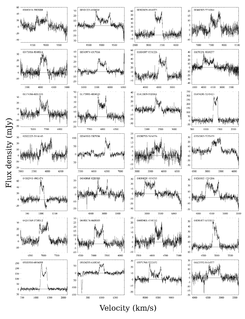
Figure 2: 28 H i spectra of Parkes observed galaxies. The 2MASS name is given at the top of each spectrum. All spectra are baseline subtracted. All 152 spectra will be available in digital form at http://ict.icrar.org/2MTF.

2.1 H i parameter measurements

2.1.1 Integrated line flux and errors

We measured integrated line flux ($F_{obs}$) from the smoothed and baseline-subtracted profiles. We manually marked the part of the spectrum where the H i emission line was present, and measured the integrated line flux within these boundaries. A line-free region was also marked, and the baseline (and noise $\sigma_{rms}$ in the spectrum) was measured in this part of the spectrum.

We adopted a jackknife method to estimate the error on the H i flux. For each galaxy, we built 100 jackknife spectra by leaving out one percent of the original data each time. All 100 jackknife spectra were then measured automatically using IDL routines, and the errors in H i flux were taken as:

$$\sigma_{J}=\left[\frac{N-1}{N}\sum^{N}_{i=1}\left(f_{i}^{J}-\overline{f}^{J}\right)^{2}\right]^{1/2},$$ (1)

where $N$ is the number of jackknife samples, $f_{i}^{J}$ is the measurement for the $i$th jackknife spectrum, and $\overline{f}^{J}=\frac{1}{N}\sum^{N}_{i=1}f_{i}^{J}$. We give a detailed description of jackknife error estimation in Appendix A.2.

2.1.2 Systemic velocities and velocity widths

Systemic velocities and velocity widths are measured by selecting two points on opposite sides of the H i emission profile. The velocity width is the velocity difference between the highest and lowest velocities ($v_{h}$ and $v_{l}$, respectively), $W=v_{h}-v_{l}$. The systemic velocity is the average of the two velocities, $V=(v_{h}+v_{l})/2$. The choice of measurement algorithm can affect accuracy, especially for the low S/N spectra. Koribalski et al. (2004) used H i widths measured at both 50% and 20% level of the peak flux density ($W_{P50}$ and $W_{P20}$). Haynes et al. (2011) adopted algorithms which measured the widths at the 50% level of each of the two peaks ($W_{2P50}$).

Separate from the question of which flux level at which to mark the two sides of the profile, there is the question of what method one uses to decide which channel corresponds to the given flux. The most commonly used method involves either starting from the two peaks of the profile and moving outwards from the centre until one finds the first channel below the desired flux threshold, or starting from the outside of the line profile, and moving inwards until one finds a channel that exceeds the flux threshold. This approach is adequate for most Tully-Fisher applications, because the S/N for most Tully-Fisher galaxies is sufficiently large that any noise along the sides of the line profile does not greatly complicate the width measurement. Nevertheless, to guard against the possibility of noisy spectra perturbing our measurements of $v_{h}$ and $v_{l}$, we favour a width measurement algorithm that involves fitting straight lines to either side of the spectral line profile.

Giovanelli et al. (1997) presented a method (first implemented in the Arecibo Observatory ANALYZ-GALPAC data reduction software) which fits a straight line to either side of the emission profile between 15% and 85% of the peak value ($f_{p}-\sigma_{rms}$), then selected the left and right points at the 50% level of the peak value from the fitted lines ($W_{F50}$). The method was later used by Springob et al. (2005), who updated the instrumental and velocity resolution correction. This represents our “favoured approach” to measuring the line width.

We measured systemic velocities and velocity widths using a modified version of the GBTIDL routine awv.pro (see Masters et al. in prep. who also use this). This routine provides H i parameter measurements using five different algorithms: $W_{F50}$ is the width measured at 50% of the value of $f_{p}-\sigma_{rms}$ on a linear fit of both sides of the profile; $W_{M50}$ is the width measured at 50% of the mean flux of the profile; $W_{2P50}$ is the width measured at 50% of each of the two $f_{p}-\sigma_{rms}$ values; $W_{P50}$ is the width measured at 50% of the $f_{p}-\sigma_{rms}$ value; and $W_{P20}$ is measured at 20% of the $f_{p}-\sigma_{rms}$ value. $W_{F50}$ is the only one of these width measurements for which $v_{h}$ and $v_{l}$ are measured by fitting a line to either side of the profile. The measurements of $v_{h}$ and $v_{l}$ for $W_{2P50}$ are made by starting at the peaks of the profile and moving outwards, while the corresponding measurements of $v_{h}$ and $v_{l}$ for $W_{M50}$, $W_{P50}$, and $W_{P20}$ are made by starting from the outside of the spectral line profile and moving inwards.

We report all five of these widths here, so comparison with results in other databases can be made. However, in this paper, we base our values for the final corrected value ($W_{c}$) on the $W_{F50}$ measurement. As Springob et al. (2005) pointed out, this reduces the dependence on the S/N of the spectra.

We applied four corrections to $W_{F50}$ to obtain $W_{c}$: the instrumental correction, the cosmological redshift correction, the correction for the turbulent motions of H i gas, and the correction for the inclination of the disk:

$$W_{c}=\left(\dfrac{W_{F50}-2\Delta_{v}\lambda}{1+z}-\Delta_{t}\right)\dfrac{1}{\sin{i}},$$ (2)

where $z$ is the redshift of the galaxy. $\Delta_{v}=3.3$ km s^-1 is the velocity resolution of the spectrum. As given by Springob et al. (2005), $\lambda$ is an empirically derived parameter for the instrumental correction that depends on the S/N and smoothing method (see §3.2.2 and Table 2 of Springob et al. (2005) for more information about this correction). $\Delta_{t}=6.5$ km s^-1 is the correction for turbulent motions (Springob et al., 2005). Finally, the inclination $i$ was estimated using the co-added axis ratio ($b/a$) from the 2MASS isophotal photometry by:

$$\cos^{2}{i}=\dfrac{(b/a)^{2}-q^{2}_{0}}{1-q^{2}_{0}},$$ (3)

where we adopt $q_{0}=0.2$ as the intrinsic axis ratio for an edge-on spiral and set $\sin{i}=1$ for objects with $b/a$ below this value.

To estimate errors in the velocity parameters, we used a Monte-Carlo method following Donley et al. (2005). Every galaxy spectrum was smoothed by a Savitzky-Golay smoothing filter. Fifty mock spectra were created for each galaxy by adding Poisson noise to the smoothed spectrum template, with the rms of the noise being equal to the rms of the original spectrum. Then the error was taken as the standard scatters of the measurements of the fifty mock spectra. We further discuss this method and compare it with other error estimating methods in the Appendix.

The errors on the $W_{F50}$ width are also corrected using Equation 7 in Giovanelli et al. (1997), which contains the uncertainties on observations and all four corrections adopted for correcting the widths. We report the corrected width error ($\epsilon_{wc}$) following the corrected widths in the final data catalog.

2.2 Catalog presentation

We present the measured parameters of 152 well-detected galaxies in Table 2. The contents of Table 2 are as follows.

Column (1). — The 2MASS XSC ID name.

Column (2) and (3). — Right ascension (RA) and declination (DEC) in the J2000.0 epoch from the 2MASS XSC.

Column (4). — The heliocentric redshift $V_{2MRS}$ from the 2MRS (km s^-1).

Column (5). — The morphological type code following the RC3 system. Classification comes from the 2MRS.

Column (6). — Co-added axis ratio ($b/a$) from the 2MASS XSC.

Column (7). — The observed integrated 21-cm H i line flux $F_{obs}$ (Jy km s^-1).

Column (8). — The uncertainty $\epsilon_{F}$ of the observed integrated H i line flux (Jy km s^-1).

Column (9). — The heliocentric systemic velocity $V_{HI}$ of the H i emission profile, generated by the fitting algorithm discussed in § 2.1.2, taken as the midpoint of the velocity at 50% level of $f_{p}-rms$, in km s^-1.

Columns (10-14). — The velocity widths of the H i line in km s^-1, using the five measuring algorithms discussed in § 2.1.2. The widths are $W_{F50}$, $W_{M50}$, $W_{2P50}$, $W_{P50}$ and $W_{P20}$ respectively.

Columns (15-29). — The observing error of five widths, estimated by the Monte-Carlo method. $\epsilon_{F50}$, $\epsilon_{M50}$, $\epsilon_{2P50}$, $\epsilon_{P50}$ and $\epsilon_{P20}$ respectively, also in km s^-1.

Column (20). — The corrected velocity width $W_{c}$, in km s^-1, which accounts for all four corrections discussed in § 2.1.2. The correction is applied to $W_{F50}$ only.

Column (21). — The uncertainty $\epsilon_{Wc}$ of the corrected velocity (km s^-1).

Column (22). — Peak signal-to-noise ratio of the H i line, $\textrm{S/N}=f_{p}/\sigma_{rms}$

Column (23). — Velocity width instrumental correction parameter, $\lambda$.

Table 2:  H i Parameters of well-detected galaxies

2MASX ID	RA	DEC	$V_{2MRS}$	$T$	$b/a$	$F_{obs}$	$\epsilon_{F}$	$V_{HI}$	$W_{F50}$	$W_{M50}$	$W_{2P50}$	$W_{P50}$	$W_{P20}$	$\epsilon_{F50}$	$\epsilon_{M50}$	$\epsilon_{2P50}$	$\epsilon_{P50}$	$\epsilon_{P20}$	$W_{c}$	$\epsilon_{Wc}$	S/N	$\lambda$
- -	[deg] (J2000)		[km s-1]	- -	- -	[Jy km s-1]		[km s-1]													- -	- -
(1)	(2)	(3)	(4)	(5)	(6)	(7)	(8)	(9)	(10)	(11)	(12)	(13)	(14)	(15)	(16)	(17)	(18)	(19)	(20)	(21)	(22)	(23)
00180131-5905008	4.5056	-59.0836	8924	4	0.30	8.92	0.87	8856	452	488	444	433	488	13	13	9	25	14	442	13.1	6.45	0.167
00301223-4106041	7.5509	-41.1012	8988	6	0.14	8.53	1.31	9066	589	601	591	582	606	3	6	4	4	7	563	3.8	10.12	0.321
00302429-4841073	7.6013	-48.6853	3352	0	0.28	11.78	0.40	3378	276	283	276	271	296	2	3	4	4	5	269	3.6	11.26	0.357
00460905-5534064	11.5376	-55.5685	7660	1	0.38	4.00	0.56	7676	396	403	397	386	409	10	6	7	5	7	401	11.4	6.11	0.149
00471816-8048016	11.8259	-80.8005	4138	1	0.36	6.03	0.25	4133	260	268	252	246	281	10	9	9	6	11	260	10.7	8.43	0.258
00543974-6317016	13.6656	-63.2838	5662	4	0.40	5.94	0.35	5710	324	335	329	320	355	4	6	5	5	9	330	6.5	10.78	0.342
01004587-8531226	15.1912	-85.5229	4657	6	0.16	10.07	0.60	4657	300	320	297	291	338	3	8	5	5	10	286	3.8	10.82	0.343
01070231-8018277	16.7593	-80.3077	5047	-2	0.32	10.66	0.58	4286	597	628	593	592	629	7	10	10	12	11	598	9.5	8.76	0.271
01374066-6051535	24.4194	-60.8649	5425	5	0.40	5.26	0.35	5411	310	310	308	306	330	3	5	4	4	7	316	6.2	8.31	0.254
01375995-4004023	24.4998	-40.0673	5985	6	0.30	8.41	0.88	5987	327	335	329	325	344	3	3	3	3	6	320	4.3	11.03	0.350
01413509-8920041	25.4056	-89.3345	2429	4	0.40	3.89	0.54	2429	229	229	226	216	232	4	4	5	5	7	233	5.6	8.32	0.254
02022225-5316145	30.5928	-53.2707	5884	3	0.24	6.44	0.55	5971	411	466	417	417	466	8	14	6	7	14	399	8.7	8.04	0.242
02043502-5507096	31.1458	-55.1193	6293	1	0.48	12.54	0.32	6529	188	194	186	185	199	2	3	2	2	3	195	5.2	15.70	0.395
03280755-5634356	52.0315	-56.5766	5797	0	0.42	2.72	0.37	5800	274	287	280	265	288	6	7	13	6	8	282	8.1	5.56	0.116
03515803-5955459	57.9918	-59.9294	5301	1	0.44	7.25	0.56	5338	349	355	346	339	390	4	13	5	6	11	364	8.3	9.47	0.298
04002940-4901474	60.1225	-49.0299	1059	1	0.44	6.34	0.37	1051	145	149	147	142	162	3	3	3	3	3	147	4.7	12.43	0.391
04040868-8220300	61.0360	-82.3417	4893	1	0.34	2.49	0.75	4950	381	403	383	377	403	4	7	5	5	7	382	5.8	7.01	0.195
04084028-4934593	62.1678	-49.5831	5421	98	0.42	7.14	0.55	5110	388	396	392	386	399	3	5	4	4	5	402	7.7	7.46	0.216
04210005-4504206	65.2502	-45.0724	4639	3	0.24	9.00	1.23	4540	493	509	490	490	518	4	5	5	4	9	481	4.8	10.46	0.332
04243569-5758512	66.1487	-57.9809	7057	4	0.48	8.29	0.74	7027	359	364	361	352	399	5	11	5	5	11	381	10.3	9.17	0.287
04480174-4608183	72.0071	-46.1385	5276	3	0.18	5.42	0.46	5203	342	346	342	342	365	3	5	4	4	8	327	3.5	9.61	0.303
04483401-4748592	72.1417	-47.8164	4316	6	0.48	3.22	0.38	4255	281	288	282	276	297	4	6	4	5	7	301	8.4	7.37	0.212
04580477-6355133	74.5200	-63.9204	4946	10	0.40	8.42	0.28	4980	264	261	267	173	275	4	3	4	22	4	268	6.4	14.72	0.395
05020500-6934058	75.5209	-69.5683	1300	5	0.30	43.41	0.44	1302	244	259	243	241	264	1	1	1	1	2	240	2.8	33.63	0.395
05024255-6108242	75.6773	-61.1401	1014	8	0.48	9.70	0.26	1014	177	186	175	175	200	4	5	6	6	6	188	6.5	8.86	0.275
05571768-5222152	89.3237	-52.3709	8505	6	0.18	5.44	1.33	8400	477	495	478	469	495	3	7	5	5	7	455	3.9	10.61	0.337
06123552-8434577	93.1474	-84.5827	4784	3	0.26	4.16	0.62	4756	444	461	443	442	469	5	7	19	7	6	435	5.7	6.84	0.187
07174094-5558355	109.4206	-55.9765	8772	4	0.40	3.24	0.56	8770	429	435	433	420	435	9	6	10	7	6	437	11.3	5.55	0.116
07284622-7436114	112.1926	-74.6032	6205	4	0.22	2.68	0.38	6253	409	422	406	405	422	5	5	5	7	5	394	5.6	6.49	0.169
07351844-5014596	113.8269	-50.2500	1200	5	0.38	15.03	0.26	1202	90	115	89	88	125	2	3	3	3	4	85	2.8	22.67	0.395
07361230-6947467	114.0514	-69.7963	1499	5	0.48	2.16	0.14	1366	108	101	108	87	114	7	6	9	9	6	111	8.2	6.87	0.189
07425487-7113095	115.7285	-71.2193	8428	5	0.46	3.32	0.85	8395	446	513	427	443	511	9	11	10	12	12	469	13.8	9.15	0.286
07441185-3548317	116.0495	-35.8088	2879	5	0.24	26.47	0.39	2889	277	300	283	262	302	1	2	3	2	2	267	2.7	28.80	0.395
07445959-7431008	116.2485	-74.5169	4832	5	0.40	3.84	0.33	4836	330	339	332	327	340	6	5	4	5	6	339	7.8	6.26	0.157
07472880-6942350	116.8700	-69.7097	4043	6	0.28	2.88	0.44	3983	328	332	333	310	335	10	7	10	12	7	322	10.5	5.53	0.114
07501902-7252285	117.5794	-72.8746	5261	3	0.46	9.34	0.48	5213	367	385	369	369	397	5	9	6	6	9	389	9.7	8.29	0.252
07581500-4951050	119.5625	-49.8514	1119	6	0.20	100.73	0.79	1117	314	323	313	310	330	1	1	1	1	2	304	2.2	31.04	0.395
08422422-7352468	130.6005	-73.8797	5097	5	0.30	5.73	0.41	5099	321	324	323	316	325	5	4	5	4	5	317	5.7	5.77	0.129
09232812-6252562	140.8672	-62.8823	4562	20	0.30	8.43	0.48	4561	278	290	274	273	304	4	6	4	5	7	273	4.5	9.58	0.302
09314981-6541445	142.9574	-65.6957	4698	4	0.44	8.98	0.53	4699	373	391	369	369	394	5	5	5	5	7	391	9.2	8.53	0.262
Table 2 is available in its entirety online. A portion is shown here for guidance regarding its form and content.

3 Data Characteristics

The sky distribution for all 152 well-detected galaxies is shown in Figure 1 by blue stars. As discussed by Springob et al. (2007), the SFI++ catalog leaves a large gap near the Galactic plane, with only a few galaxies included in the region $|b|<15^{\circ}$. Thus, a significant number of our Parkes observations were focused on this low Galactic latitude area where we provide 69 high-accuracy H i measurements. Note that even in the NIR, dust obscuration and stellar crowding still leave a small ZoA at Galactic latitudes $|b|<5^{\circ}$.

Figure 3 shows the H i systemic velocity distribution of the 152 galaxies. As discussed in Section 2, we limited our sample to $cz<10,000$ km s^-1to get better H i profiles. Of the 152 measured systemic velocities, 121 (about 80%) are less than 6,000 km s^-1, with a mean value of 152 systemic velocities $\overline{V_{HI}}=4433$ km s^-1. The highest-velocity galaxy is at $cz=9066$ km s^-1, and the nearest one is at $cz=524$ km s^-1.

Figure 3: The systemic velocity distributions of the 152 high quality Parkes galaxies, in bins of width $500$ km s^-1.

The distribution of the differences between 2MRS and H i systemic velocities is shown in Figure 4.

Figure 4: $V_{HI}$-$V_{2MRS}$ versus $V_{2MRS}$ plot of 152 galaxies. The scatter about the line is 77 km s^-1.

The distributions of the peak signal-to-noise ratio ($\textrm{S/N}=f_{p}/\sigma_{rms}$) and rms are shown in Figure 5 and Figure 6 respectively. All galaxies have a $\textrm{S/N}>5$, and 66 S/Ns are larger than 10. Generally, for the IDL routines we used to reduce the Parkes H i data, a S/N larger than five appears to be sufficient to measure an accurate width.

Figure 5: The distribution of peak Signal-to-Noise ratio of the 152 high quality Parkes galaxies, in bins of width 0.1 dex in logarithmic space.

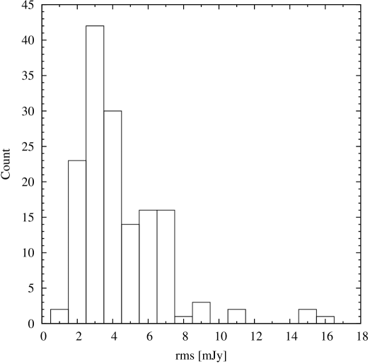
Figure 6: The distribution of rms of the 152 high quality Parkes galaxies, in bins of width 1 mJy.

Figure 7 shows the distribution of the observed integrated H i flux $F_{obs}$. Compared to the catalog presented by Springob et al. (2005), our sample detects galaxies with larger integrated H i flux, because of the source selection criteria and the limit of telescope sensitivity. As indicated by the Figure 7, the distribution of H i flux shows a peak at $\sim 7$ Jy km s^-1, with a mean value of $\overline{F_{obs}}=12.4$ Jy km s^-1.

Figure 7: The distribution of integrated H i flux for 152 galaxies, in bins of width 0.1 dex.

Figure 8: The distributions of corrected widths, absolute errors of corrected widths and relative errors, in bins of 50 km s^-1, 1 km s^-1and 0.5% respectively.

Finally, we show the histograms for the corrected widths $W_{c}$ and the errors of corrected widths $\epsilon_{Wc}$ in Figure 8. In comparison to the catalog of the 1000 brightest HIPASS galaxies, our catalog includes faster rotators, again mainly because of the selection criteria. For the 2MTF project, whose final goal is estimating the redshift-independent distances for spiral galaxies, the accuracy of H i width is one of the most important target parameters. All but four of the galaxies have relative width errors below 5%: the profiles of 2MASX 07361230-6947467 and 12541830-4149141 have $\textrm{S/N}\sim 6$; 2MASX 14242324-8027573 has a well-measured profile ($\textrm{S/N}>10$) but its slow rotation ($W_{c}=74$ km s^-1) amplifies the relative error; 2MASX 01474280-5245423 has an excellent profile ($\textrm{S/N}\sim 18$) but its unfavorable inclination ($b/a=0.8$) causes a very large uncertainty in the width. As the latter galaxy has $b/a>0.5$, it is eliminated from further cosmological analysis.

4 Notable Detections

4.1 Discrepant Velocities

We compared our derived H i systemic velocities with those listed in the NASA/IPAC Extragalactic Database (NED) and found 5 objects that are discrepant by more than $3\sigma$, as listed below:

(i) 2MASX 01070231-8018277: NED prefers $cz=5047\pm 21$ km s^-1(Lauberts & Valentijn, 1989), but also lists $cz=4145\pm 27$ km s^-1(Wegner et al., 2003) and $cz=4249\pm 27$ km s^-1(da Costa et al., 1991). We determined $V_{HI}=4286\pm 4$ km s^-1, thus confirming the alternate velocities.

(ii) 2MASX 18363723-4703153: NED prefers $cz=7005\pm 29$ km s^-1(Huchra et al., 2012). We determined $V_{HI}=6824\pm 1$ km s^-1, in agreement with $cz=6857\pm 45$ km s^-1from the 6dF Galaxy Survey (6dFGS, Jones et al., 2009).

(iii) 2MASX 20453927-5826591: NED prefers $cz=6954\pm 45$ km s^-1(Jones et al., 2009), but also lists $cz=7105\pm 89$ km s^-1from the 2dF Galaxy Redshift Survey catalog (2dFGRS) . We determined $V_{HI}=7090\pm 2$ km s^-1, in better agreements with the 2dFGRS value.

(iv) 2MASX 16375253-6448486: NED prefers $cz=4900\pm 70$ km s^-1(di Nella et al., 1997). We determined $V_{HI}=4688\pm 1$ km s^-1which agrees with the HIPASS velocity (Doyle et al., 2005) of $cz=4693$ km s^-1.

(v) 2MASX 02043502-5507096: NED prefers $cz=6293\pm 31$ km s^-1(Huchra et al., 2012), but we determined $V_{HI}=6529\pm 1$ km s^-1.

4.2 Non-detected galaxies

Limited by the observing time on the Parkes telescope, our observation plan mainly focused on the galaxies which had a HIPASS peak flux density larger than 20 mJy. Of the 303 observed galaxies, only 152 galaxies were well-detected with good spectra which meet the requirements for accurate Tully-Fisher distance estimation. We cross-matched the non-detected list with the HIPASS galaxy catalog, and list these galaxies in Table 3 for reference.

Table 3: Non-detected Galaxies

2MASX ID	RA (J2000)	DEC (J2000)	$V_{2MRS}$	rms	Flag
	[deg]	[deg]	[km s-1]	[mJy]
(1)	(2)	(3)	(4)	(5)	(6)
00011748-5300348	0.3228	-53.0097	9724	5.20	N
00032138-5004494	0.8390	-50.0805	10333	8.50	N
00034062-4951278	0.9194	-49.8578	8327	7.12	N
00054271-7542251	1.4278	-75.7070	6028	8.19	N
00182593-8306394	4.6081	-83.1110	4534	6.84	Y
00254881-6219480	6.4533	-62.3300	9174	8.53	N
00543231-4042578	13.6347	-40.7161	7273	7.84	N
00571478-4057329	14.3116	-40.9591	3397	7.40	Y
01004798-5148563	15.1999	-51.8156	7449	8.07	N
01013572-5312020	15.3988	-53.2005	7457	7.59	N
01071459-4637191	16.8109	-46.6220	6081	7.52	Y
01093909-6119597	17.4128	-61.3332	7891	3.79	Y
01101993-4551184	17.5830	-45.8551	6968	7.45	Y
01281188-4334337	22.0496	-43.5760	9774	7.94	Y
01284236-5124573	22.1766	-51.4160	9068	7.10	N

Notes –	Y: One or more peaks with flux $S_{peak}\geqslant 20$ mJy is found on the HIPASS spectrum in the velocity region of $V_{2MRS}\pm 200$ km s-1.
	N: No peaks with flux $S_{peak}\geqslant 20$ mJy are found on the HIPASS spectrum in the velocity region of $V_{2MRS}\pm 200$ km s-1.
Table 3 is available in its entirety online. A portion is shown here for guidance regarding its form and content.

5 Summary

We observed 303 galaxies in the southern hemisphere ($\delta<-40^{\circ}$), as a part of the 2MASS Tully-Fisher survey, using the Parkes radio telescope with the 21-cm multibeam receiver. The velocity resolution of raw spectra is 1.6 km s^-1, after the 3 channel Hanning smoothing during the data reduction process, The final velocity resolution after Hanning smoothing is 3.3 km s^-1. All galaxies were selected from the 2MRS catalog with limits of $K_{s}<11.25$ mag, $cz<10,000$ km s^-1, and axis ratio $b/a<0.5$.

152 galaxies were detected with high quality spectra. We have presented a table of both H i spectral parameters and corrected rotational velocities for these galaxies. All 152 galaxies have $\textrm{S/N}>5$, and 66 have $\textrm{S/N}>10$. We carefully measured the H i spectral parameters using a similar method to that applied to the 2MTF GBT and Arecibo data, and converted the linewidths to rotational velocities, which will be used for calculating the Tully-Fisher distances. We measured velocity widths with better than 5% precision (suitable for application of the Tully-Fisher relation) for 148 out of 152 galaxies.

These observation comprise the southern portion of 2MTF and provide 69 high-accuracy measurements of galaxies in the southern Zone of Avoidance ($|b|<15^{\circ}$). The improved uniformity and completeness will result in more accurate determinations of local peculiar velocities.

We gratefully acknowledge help with Parkes Observations from John Huchra, Stacy Mader, A. Kels, Danny Price, Emma Kirby, Christina Magoulas and Vicky Safouris and all of the CSIRO staff at Parkes Observatory. The authors wish particularly to acknowledge John Huchra (1948-2010), without whose vision 2MTF would never have happened. The 2MTF survey was initiated while KLM was a postdoc working with JPH at Harvard, and its design owes much to the insight and advice of JPH.

Parts of this research were conducted by the Australian Research Council Centre of Excellence for All-sky Astrophysics (CAASTRO), through project number CE110001020. TH was supported by the National Natural Science Foundation (NNSF) of China (10833003 and 11103032). KLM was supported by NSF grant AST-0406906, the Peter and Patricia Gruber Foundation, and the Leverhulme Trust. LMM was supported by NASA through Hubble Fellowship grant HST-HF-01153 from the Space Telescope Science Institute and by the NSF through a Goldberg Fellowship from the National Optical Astronomy Observatory. ACC was supported by NSF grant AST-0406906.

Appendix A Errors in H i parameters

To estimate the errors on the H i parameters, we used two different methods. A Monte-Carlo method was used for the errors of line widths and central velocities, and a jackknife method was adopted for the errors in flux. We describe these two methods in this section. We also compare the errors estimated by both methods with the errors estimated by the method of the HIPASS Brightest Galaxy Catalog (HIPASS BGC method).

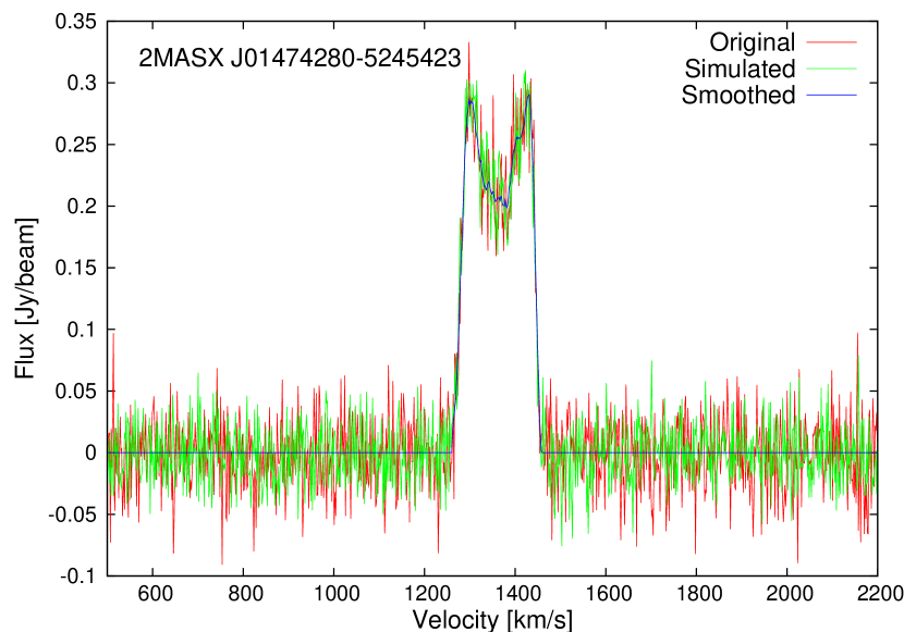
Figure 9: The spectrum of galaxy 2MASX J01474280-5245423, together with the smoothed and mock spectrum. The red line indicates the original spectrum, the blue line shows the smoothed spectrum using a 17-point Savitzky-Golay smoothing filter, and the green line is the mock spectrum created by adding Poisson noise to the smoothed spectrum.

A.1 The Monte-Carlo method

We adopted a Monte-Carlo method to estimate the errors in the H i velocity parameters. Firstly, we smoothed each galaxy spectrum using a 17-point Savitzky-Golay smoothing filter (Press et al., 2002, §14.8). This low-pass filter can significantly reduce the noise while keeping high order features of the spectrum. Fifty mock spectra were then created for every galaxy by adding Poisson noise to the smoothed spectrum. The rms of the random noise was equal to the rms of the original galaxy spectrum. These mock spectra were measured with an automatic IDL routine, based on the IDL routine awv.pro. The standard errors of the measurements of the fifty mock spectra were then taken as the errors of the H i parameters. Figure 9 shows the smoothed and mock spectrum of galaxy 2MASX J01474280-5245423 as an example.

Donley et al. (2005) adopted a similar analysis for the Parkes Zone of Avoidance (ZoA) survey, and found this Monte-Carlo method worked well for high S/N spectra while the errors became unreliable for $\textrm{S/N}<5$. For the 152 well-detected galaxies in our sample, all galaxies have a peak $\textrm{S/N}>5$. 86 have $5<\textrm{S/N}\leqslant 10$, and 66 have $\textrm{S/N}>10$.

Figure 10: The comparison plot of human-measured and machine-measured H i $W_{F50}$ widths. The solid line indicates equality. The scatter of these two measurements is about 2 km s^-1.

A.2 The jackknife method

The Monte-Carlo method operates on the spectra following baseline correction. Since baseline correction is one of the major sources of error for the measurement of H i flux, we have adopted an alternative jackknife method to estimate the errors in H i flux. After bandpass and Doppler correction with livedata, we repeated the gridding and baseline fitting process using an IDL routine instead of the gridzilla. As mentioned in Section 2, the correlator writes a spectrum every 5 seconds for each polarization. Thus in a standard 35 mins integration, 940 ‘sub-spectra’ are recorded.

We built 100 jackknife spectra for every galaxy by removing 4 different polarization pairs of sub-spectra from the original data and adding the rest of the spectra together using the MEDIAN method.

All the jackknife spectra were measured automatically using the same IDL routines used in Section A.1. Finally, we obtain the jackknife estimate of the flux error from Equation 1.

A.3 Reliability of the machine-measured H i properties

We compare the estimates of manual measurements with the mean value of machine-measured H i widths, to make sure our automatic routine can measure the H i profiles correctly. The comparison for our preferred $W_{F50}$ widths is plotted in Figure 10, and shows no significant systematic offset between manual and machine-measured $W_{F50}$ widths.

A.4 Comparison with the HIPASS BGC method

Koribalski et al. (2004) estimated the errors of the 1000 brightest HIPASS galaxies using:

$$\sigma(v_{sys})=3(S/N)^{-1}(P\Delta_{v})^{1/2}$$ (4)

$$\sigma(w_{50})=2\sigma(v_{sys}),$$ (5)

$$\sigma\left(F_{HI}\right)=4\left(S/N\right)^{-1}\left(S_{peak}F_{HI}\Delta_{v}\right)^{1/2},$$ (6)

where S/N is the signal-to-noise ratio, $S_{peak}$ is the peak flux density, $\Delta_{v}=3.3$ km s^-1 is the velocity resolution, and $P=0.5(w_{20}-w_{50})$ indicates the slope of the H i profile.

Firstly we compared the $W_{F50}$ width errors estimated by the Monte-Carlo method with the errors calculated by Equation 5 (Figure 11). These two methods are consistent. However, we find that the HIPASS BGC method tends to slightly overestimate the width errors.

Figure 11: Comparison of the Monte-Carlo width errors and the errors estimated using HIPASS BGC method. The solid line indicates the line of y=x.

We also compared the flux error which was estimated using the jackknife method with the errors of HIPASS BGC method (Figure 12).

Figure 12: Comparison of the jackknife flux errors and the errors estimated using the HIPASS BGC method. The solid line indicates the line of y=x.

These two methods agree with each other, but with a large scatter, especially for some low signal-to-noise ratio spectra. Our jackknife method is more sensitive to the S/N than HIPASS BGC method, the jackknife gave very large flux errors for low S/N galaxies. However, for well observed galaxies, the two methods provide similar values.

References

- Aaronson et al. (1982) Aaronson, M., Huchra, J., Mould, J., Schechter, P. L., & Tully, R. B. 1982, ApJ, 258, 64
- Barnes et al. (2001) Barnes, D. G., Staveley-Smith, L., de Blok, W. J. G., et al. 2001, MNRAS, 322, 486
- da Costa et al. (1991) da Costa, L. N., Pellegrini, P. S., Davis, M., et al. 1991, ApJS, 75, 935
- de Lapparent et al. (1986) de Lapparent, V., Geller, M. J., & Huchra, J. P. 1986, ApJL, 302, L1
- di Nella et al. (1997) di Nella, H., Couch, W. J., Parker, Q. A., & Paturel, G. 1997, MNRAS, 287, 472
- Donley et al. (2005) Donley, J. L., Staveley-Smith, L., Kraan-Korteweg, R. C., et al. 2005, AJ, 129, 220
- Doyle et al. (2005) Doyle, M. T., Drinkwater, M. J., Rohde, D. J., et al. 2005, MNRAS, 361, 34
- Erdoğdu et al. (2006) Erdoğdu, P., Lahav, O., Huchra, J. P., et al. 2006, MNRAS, 373, 45
- Giovanelli et al. (1997) Giovanelli, R., Haynes, M. P., Herter, T., et al. 1997, AJ, 113, 22
- Giovanelli et al. (2005) Giovanelli, R., Haynes, M. P., Kent, B. R., et al. 2005, AJ, 130, 2598
- Haynes et al. (1999a) Haynes, M. P., Giovanelli, R., Chamaraux, P., et al. 1999a, AJ, 117, 2039
- Haynes et al. (1999b) Haynes, M. P., Giovanelli, R., Salzer, J. J., et al. 1999b, AJ, 117, 1668
- Haynes et al. (2011) Haynes, M. P., Giovanelli, R., Martin, A. M., et al. 2011, AJ, 142, 170
- Hong et al. (2013) Hong, T., Staveley-Smith, L., Masters, K., et al. 2013, in IAU Symposium, Vol. 289, IAU Symposium, ed. R. de Grijs, 312–315
- Huchra et al. (2012) Huchra, J. P., Macri, L. M., Masters, K. L., et al. 2012, ApJS, 199, 26
- Jarrett et al. (2000) Jarrett, T. H., Chester, T., Cutri, R., et al. 2000, AJ, 119, 2498
- Jones et al. (2009) Jones, D. H., Read, M. A., Saunders, W., et al. 2009, MNRAS, 399, 683
- Koribalski et al. (2004) Koribalski, B. S., Staveley-Smith, L., Kilborn, V. A., et al. 2004, AJ, 128, 16
- Lauberts & Valentijn (1989) Lauberts, A., & Valentijn, E. A. 1989, The surface photometry catalogue of the ESO-Uppsala galaxies
- Masters (2008) Masters, K. L. 2008, in Astronomical Society of the Pacific Conference Series, Vol. 395, Frontiers of Astrophysics: A Celebration of NRAO’s 50th Anniversary, ed. A. H. Bridle, J. J. Condon, & G. C. Hunt, 137
- Masters et al. (2006) Masters, K. L., Springob, C. M., Haynes, M. P., & Giovanelli, R. 2006, ApJ, 653, 861
- Masters et al. (2008) Masters, K. L., Springob, C. M., & Huchra, J. P. 2008, AJ, 135, 1738
- Press et al. (2002) Press, W. H., Teukolsky, S. A., Vetterling, W. T., & Flannery, B. P. 2002, Numerical recipes in C++ : the art of scientific computing
- Scrimgeour et al. (2012) Scrimgeour, M. I., Davis, T., Blake, C., et al. 2012, MNRAS, 425, 116
- Springob et al. (2005) Springob, C. M., Haynes, M. P., Giovanelli, R., & Kent, B. R. 2005, ApJS, 160, 149
- Springob et al. (2007) Springob, C. M., Masters, K. L., Haynes, M. P., Giovanelli, R., & Marinoni, C. 2007, ApJS, 172, 599
- Staveley-Smith et al. (1996) Staveley-Smith, L., Wilson, W. E., Bird, T. S., et al. 1996, PASA, 13, 243
- Theureau et al. (1998) Theureau, G., Bottinelli, L., Coudreau-Durand, N., et al. 1998, A&AS, 130, 333
- Theureau et al. (2005) Theureau, G., Coudreau, N., Hallet, N., et al. 2005, A&A, 430, 373
- Tully & Courtois (2012) Tully, R. B., & Courtois, H. M. 2012, ApJ, 749, 78
- Tully & Fisher (1977) Tully, R. B., & Fisher, J. R. 1977, A&A, 54, 661
- Tully et al. (2008) Tully, R. B., Shaya, E. J., Karachentsev, I. D., et al. 2008, ApJ, 676, 184
- Wegner et al. (2003) Wegner, G., Bernardi, M., Willmer, C. N. A., et al. 2003, AJ, 126, 2268