Coexistence of Near-Field and Far-Field Sources: the Angular Resolution Limit

Abstract

Passive source localization is a well known inverse problem in which we convert the observed measurements into information about the direction of arrivals. In this paper we focus on the optimal resolution of such problem. More precisely, we propose in this contribution to derive and analyze the Angular Resolution Limit (ARL) for the scenario of mixed Near-Field (NF) and Far-Field (FF) Sources. This scenario is relevant to some realistic situations. We base our analysis on the Smith’s equation which involves the Cramér-Rao Bound (CRB). This equation provides the theoretical ARL which is independent of a specific estimator. Our methodology is the following: first, we derive a closed-form expression of the CRB for the considered problem. Using these expressions, we can rewrite the Smith’s equation as a 4-th order polynomial by assuming a small separation of the sources. Finally, we derive in closed-form the analytic ARL under or not the assumption of low noise variance. The obtained expression is compact and can provide useful qualitative informations on the behavior of the ARL.

1 Introduction

Very few works are related to the study of the realistic situation where there exists coexisting far-field (FF) and near-field (NF) sources [2] such as speaker localization using microphone arrays and guidance (homing) systems. At the contrary, we can find a plethora of contributions on the localization of far-field sources [1]. More recently, the problem of localization of near-field sources has been tackled in reference [4, 5] for instance. In the context of the problem of source localization, one can see three contributions: (1) propose new efficient algorithms/estimators [1], (2) study the estimation performance independently of a specific algorithm thanks to the lower bound on the Mean Square error (MSE) [3, 5] and (3) derive and study the theoretical resolution, i.e., the minimal angular distance to resolve/discriminate two closely spaced emitted signals in terms of their direction of arrivals. Our contribution belongs to the third point. More precisely, based on the Smith’s equation [6, 8, 9] which involves the Cramér-Rao Bound (CRB) [3], we derive and analyze the Angular Resolution Limit (ARL) for the realistic scenario where we have two sources, one located in the far-field of the array and another in the near-field of the array.

2 Model setup

We consider some practical applications where the signals $s_{1}(t)$ and $s_{2}(t)$ with $t\in[1:T]$ in which $T$ is the number of snapshots received by an uniform linear array composed by $L$ sensors are the mixture of near-field and far-field sources. More precisely, the $(TL)\times 1$ observation vector is defined as ${\bf y}={\bf\bar{y}}+{\bf e}$ where ${\bf e}$ is the complex centered circular additive white Gaussian noise of variance $\sigma^{2}$ and the $(TL)\times 1$ noise-free signal is ${\bf\bar{y}}=\begin{bmatrix}{\bf A}{\bf s}(1)\\ \vdots\\ {\bf A}{\bf s}(T)\end{bmatrix}$ with ${\bf s}(t)=[s_{1}(t)\ s_{2}(t)]^{T}$ and ${\bf A}=\begin{bmatrix}{\bf a}(\omega_{1})&{\bf b}(\omega_{2},\phi)\end{bmatrix}$ where the signal sources $s_{m}(t)$ are viewed as deterministic known signals and the steering vectors are defined by $[{\bf a}(\omega_{1})]_{\ell}=e^{i\omega_{1}\ell}$ and $[{\bf b}(\omega_{2},\phi)]_{\ell}=e^{i(\omega_{2}\ell+\phi\ell^{2})}$ with $\ell\in[0:L-1]$. In addition, we assume $\omega_{1}\neq\omega_{2}$. We define the determinist non-zero separation by $\delta=\omega_{2}-\omega_{1}$. We focus our attention on the electric parameters but these parameters can be linked to the physical parameters, namely the DOA $\theta_{m}$ and the range $r$, according to $\omega_{m}=-2\pi d/\lambda\sin(\theta_{m})$ and $\phi=\pi d^{2}/(\lambda r)\cos(\theta_{2})^{2}$ where $d$ is the distance inter-sensor and $\lambda$ is the wavelength.

3 Analytic ARL in the Smith’s sense

3.1 Analytical expression of the Cramer-Rao Bound

The Cramer-Rao Bound (CRB) verifies the covariance inequality principle [3]. This bound is largely used in the signal processing community since it gives the best performance in term of Mean Square Error (MSE) at high Signal to Noise Ratio (SNR). Let $\hat{\omega}_{m}$ be an unbiased estimate of $\omega_{m}$, then

$$E\{(\omega_{m}-\hat{\omega}_{m})^{2}\}\geq[{\bf C}]_{mm}\stackrel{{\scriptstyle\rm def}}{{=}}[{\bf J}^{-1}]_{mm}$$ (1)

where $E\{.\}$ is the mathematical expectation and ${\bf J}$ is the Fisher Information Matrix (FIM) defined by the Slepian-Bangs formula for a complex circular Gaussian observation ${\bf y}\sim\mathcal{CN}({\bf\bar{y}},\sigma^{2}{\bf I})$:

$$[{\bf J}]_{ij} = \frac{2}{\sigma^{2}}\Re\left\{\left(\frac{\partial{\bf\bar{y}}}{\partial\omega_{i}}\right)^{H}\frac{\partial{\bf\bar{y}}}{\partial\omega_{j}}\right\}=\frac{2}{\sigma^{2}}\sum_{t=1}^{T}\Re\left\{{\bf s}(t)^{H}\left(\frac{\partial{\bf A}}{\partial\omega_{i}}\right)^{H}\frac{\partial{\bf A}}{\partial\omega_{j}}{\bf s}(t)\right\}$$ (2)

where $\frac{\partial{\bf A}}{\partial\omega_{1}}=\begin{bmatrix}{\bf\dot{a}}(\omega_{1})&{\bf 0}\end{bmatrix}$, $\frac{\partial{\bf A}}{\partial\omega_{2}}=\begin{bmatrix}{\bf 0}&{\bf\dot{b}}(\omega_{2},\phi)\end{bmatrix}$, $\frac{\partial{\bf A}}{\partial\phi}=\begin{bmatrix}{\bf 0}&{\bf\ddot{b}}(\omega_{2},\phi)\end{bmatrix}$ where ${\bf\dot{a}}(\omega_{1})$ (resp. ${\bf\dot{b}}(\omega_{2},\phi)$) is the first-order derivative of ${\bf a}(\omega_{1})$ (resp. ${\bf b}(\omega_{2},\phi)$) w.r.t. the parameters $\omega_{1}$, $\omega_{2}$, respectively and ${\bf\ddot{b}}(\omega_{2},\phi)$ is the first-order derivative w.r.t. the parameter $\phi$. After some algebra, one obtains the CRB for the parameters of interest and the coupling term:

$$\mbox{CRB}(\omega_{1}) = \frac{\sigma^{2}}{2}\frac{\beta}{\mathcal{Q}},$$ (3)

$$\mbox{CRB}(\omega_{2}) = \frac{\sigma^{2}}{2}\frac{L_{2}||{\bf s}_{1}||^{2}-\frac{\eta^{2}(\delta)}{L_{3}||{\bf s}_{2}||^{2}}}{\mathcal{Q}},$$ (4)

$$\mbox{CRB}(\omega_{1},\omega_{2}) = -\frac{\sigma^{2}}{2}\frac{\zeta(\delta)-\frac{\eta(\delta)L_{3}}{L_{4}}}{\mathcal{Q}}.$$ (5)

where $\beta=||{\bf s}_{2}||^{2}\left(L_{2}-\frac{L_{3}^{2}}{L_{4}}\right)$, $\mathcal{Q}=\beta\left(L_{2}||{\bf s}_{1}||^{2}-\frac{\eta^{2}(\delta)}{L_{3}||{\bf s}_{2}||^{2}}\right)-\left(\zeta(\delta)-\eta(\delta)\frac{L_{2}}{L_{3}}\right)^{2}$, $L_{r}=\sum_{\ell=0}^{L-1}\ell^{r}$ and $\eta(\delta)=\Re\left\{h\sum_{\ell=0}^{L-1}\ell^{2}e^{i(\delta\ell+\phi\ell^{2})}\right\}$ and $\eta(\delta)=\Re\left\{h\sum_{\ell=0}^{L-1}\ell^{3}e^{i(\delta\ell+\phi\ell^{2})}\right\}$ with $h={\bf s}_{1}^{H}{\bf s}_{2}$.

3.2 Derivation of the analytic ARL

3.2.1 The Smith’s equation:

The Smith’s methodology [6] provides the ARL as the solution of the following equation:

$$\mbox{CRB}(\delta)=\delta^{2}.$$ (6)

Expanding $\mbox{CRB}(\delta)$ w.r.t. the localization parameters and the coupling term, we have [7]:

$$\mbox{CRB}(\delta)=\mbox{CRB}(\omega_{1})+\mbox{CRB}(\omega_{2})-2\mbox{CRB}(\omega_{1},\omega_{2})$$ (7)

where the CRBs are given by expressions (3)-(5).

3.2.2 Polynomial resolution of the linearized problem:

Solving analytically equation (6) with (7) and (3)-(5) seems an intractable problem. Recalling that we assume that the separation $\delta$ is small then a first-order Taylor expansions of $\zeta(\delta)$ and $\eta(\delta)$ lead to the following approximations:

$$\eta(\delta)\approx\Re\left\{h(v(\phi)+j\delta r(\phi))\right\},\ \ \zeta(\delta)\approx\Re\left\{h(u(\phi)+j\delta v(\phi))\right\}$$ (8)

in which $u(\phi)=\sum_{\ell=0}^{L-1}\ell^{2}e^{i\phi\ell^{2}}$, $v(\phi)=\sum_{\ell=0}^{L-1}\ell^{3}e^{i\phi\ell^{2}}$ and $r(\phi)=\sum_{\ell=0}^{L-1}\ell^{4}e^{i\phi\ell^{2}}$. The above relation can be rewritten in a linear form w.r.t. the separation according to

$$\Re\left\{h(v(\phi)+j\delta r(\phi))\right\}=P-\delta Q,\ \ \Re\left\{h(u(\phi)+j\delta v(\phi))\right\}=P^{\prime}-\delta Q^{\prime}$$ (9)

where $P=\Re\{hv(\phi)\}$, $Q=-\Im\{hr(\phi)\}$, $P^{\prime}=\Re\{hu(\phi)\}$ and $Q^{\prime}=-\Im\{hv(\phi)\}$. Using these approximations, one can rewrite the CRB as

$${\bf C}={\bf J}^{-1}\stackrel{{\scriptstyle\rm def}}{{=}}\frac{\sigma^{2}}{2}\begin{bmatrix}{\bf Q}^{-1}&\times\\ \times&\times\end{bmatrix},$$ (10)

where, the Schur complement can be approximated as follow ${\bf Q}\approx\begin{bmatrix}P_{2}(\delta)&P_{1}(\delta)\\ P_{1}(\delta)&\beta\end{bmatrix}$ in which we have introduced the two following polynomials $P_{2}(\delta)=\alpha_{1}\delta+\alpha_{0}$ and $P_{2}(\delta)=a_{2}\delta^{2}+a_{1}\delta+a_{0}$ where $a_{2}=-\frac{Q^{2}}{L_{4}||{\bf s}^{2}||^{2}}$, $a_{1}=-\frac{2PQ}{L_{4}||{\bf s}^{2}||^{2}}$, $a_{0}=L_{2}||{\bf s}_{1}||^{2}-\frac{P^{2}}{L_{4}||{\bf s}^{2}||^{2}}$, $\alpha_{1}=Q^{\prime}-\frac{L_{3}}{L_{4}}Q$ and $\alpha_{0}=P^{\prime}-\frac{L_{3}}{L_{4}}P$. The linearized CRB expressions are now given by

$$\mbox{CRB}(\omega_{1})\approx\frac{\sigma^{2}}{2}\frac{\beta}{Q(\delta)},$$ (11)

$$\mbox{CRB}(\omega_{2})\approx\frac{\sigma^{2}}{2}\frac{P_{2}(\delta)}{Q(\delta)},$$ (12)

$$\mbox{CRB}(\omega_{1},\omega_{2})\approx-\frac{\sigma^{2}}{2}\frac{P_{1}(\delta)}{Q(\delta)},$$ (13)

where $Q(\delta)=P_{2}(\alpha)\beta-P_{1}^{2}(\delta)=(\beta a_{2}-\alpha_{1}^{2})\delta^{2}+(\beta a_{1}-2\alpha_{0}\alpha_{1})\delta+\beta a_{0}-\alpha_{0}^{2}$. Consequently from (6) and (11)-(13), the Smith’s equation becomes $\delta^{2}=\frac{Q^{\prime}(\delta)}{Q(\delta)}$ where $Q^{\prime}(\delta)=\frac{\sigma^{2}}{2}(\beta+P_{2}(\delta)+2P_{1}(\delta))\stackrel{{\scriptstyle\rm def}}{{=}}c_{2}\delta^{2}+c_{1}\delta+c_{0}$ with $c_{2}=\frac{\sigma^{2}}{2}a_{2}$, $c_{1}=\frac{\sigma^{2}}{2}(a_{1}+2\alpha_{1})$ and $c_{0}=\frac{\sigma^{2}}{2}(\beta+a_{0}+2\alpha_{0})$. So, it is easy to see that the Smith’s equation provides the ARL as the solution of a 4-th order polynomial according to

$$R(x)=Q(x)x^{2}-Q^{\prime}(x)\stackrel{{\scriptstyle\rm def}}{{=}}x^{4}+g_{3}x^{3}+g_{2}x^{2}+g_{1}x+g_{0}$$ (14)

where $x$ is a free variable with $g_{0}=-\frac{c_{0}}{\beta a_{2}-\alpha_{1}^{2}},$ $g_{1}=-\frac{c_{1}}{\beta a_{2}-\alpha_{1}^{2}}$, $g_{2}=\frac{\beta a_{0}-\alpha_{0}^{2}-c_{2}}{\beta a_{2}-\alpha_{1}^{2}},$ $g_{3}=\frac{\beta a_{1}-2\alpha_{0}\alpha_{1}}{\beta a_{2}-\alpha_{1}^{2}}$ where we assume $\beta a_{2}\neq\alpha_{1}^{2}$.

3.2.3 Analytic solutions of $R(x)$:

The resolution of a 4-th order polynomial is not straightforward but we propose a solution to this problem. More precisely, as $\mbox{CRB}(\delta)=\mbox{CRB}(-\delta)$, it is easy to see that if $\delta$ is a solution of the Smith’s equation then $-\delta$ is also a solution. This implies that if $\delta$ is a root of $R(x)$ then $-\delta$ is also a root. So, $R(x)$ has four roots, namely $\{\delta,-\delta,r_{1},r_{2}\}$ and a decomposition of this polynomial into a product of monomial terms is given by

$$R(x) = (x-\delta)(x+\delta)(x-r_{1})(x-r_{2})$$ (15)

$$= x^{4}-(r_{1}+r_{2})x^{3}+(r_{1}r_{2}-\delta^{2})x^{2}$$ (16)

$$+ \delta^{2}(r_{1}+r_{2})x-r_{1}r_{2}\delta^{2}.$$ (17)

We can identify the coefficients of the polynomials (14) and (17) according to

$$\left\{\begin{array}[]{ccc}-(r_{1}+r_{2})&=&\frac{\beta a_{1}-2\alpha_{0}\alpha_{1}}{\beta a_{2}-\alpha_{1}^{2}},\\ r_{1}r_{2}-\delta^{2}&=&\frac{\beta a_{0}-\alpha_{0}^{2}-c_{2}}{\beta a_{2}-\alpha_{1}^{2}},\\ \delta^{2}(r_{1}+r_{2})&=&-\frac{c_{1}}{\beta a_{2}-\alpha_{1}^{2}},\\ -r_{1}r_{2}\delta^{2}&=&-\frac{c_{0}}{\beta a_{2}-\alpha_{1}^{2}}.\end{array}\right.$$ (22)

Combining the second and the last equations, we have to solve the following polynomial:

$$R^{\prime}(x)=(\beta a_{2}-\alpha_{1}^{2})x^{4}+(\beta a_{0}-\alpha_{0}^{2}-c_{2})x^{2}-c0.$$ (23)

Polynomial $R^{\prime}(x)$ can be reformulated as a 2-rd order polynomial according to

$$R^{\prime}(z)=(\beta a_{2}-\alpha_{1}^{2})z^{2}+(\beta a_{0}-\alpha_{0}^{2}-c_{2})z-c0.$$ (24)

The discriminant is

$$\Delta=(\beta a_{0}-\alpha_{0}^{2}-c_{2})^{2}\left(1+4\frac{(\beta a_{2}-\alpha_{1}^{2})c_{0}}{(\beta a_{0}-\alpha_{0}^{2}-c_{2})^{2}}\right).$$ (25)

The study of the sign of the discriminant is not straightforward but observe that $c_{0},c_{2}\stackrel{{\scriptstyle\sigma^{2}\rightarrow 0}}{{\longrightarrow}}0$, so if the noise variance is low then the discriminant is given by

$$\Delta\stackrel{{\scriptstyle\sigma^{2}\rightarrow 0}}{{\longrightarrow}}(\beta a_{0}-\alpha_{0}^{2}-c_{2})^{2}\geq 0.$$ (26)

So, we know that if the noise variance is not too high, there exists two candidates for the ARL (or a double solution if the discriminant is zero) which are given by

$$\delta=\sqrt{\frac{-(\beta a_{0}-\alpha_{0}^{2}-c_{2})\pm\sqrt{\Delta}}{2(\beta a_{2}-\alpha_{1}^{2})}}$$ (27)

where $\sqrt{\Delta}$ is given by the square root of expression (25).

3.2.4 Analytic expression of the ARL:

To discriminate the two possible solutions, we advocate that $\delta\stackrel{{\scriptstyle\sigma^{2}\rightarrow 0}}{{\longrightarrow}}0$ is a reasonable property. Thus, note thanks to (26), the sign in (27) must be chosen as positive to ensure $\delta\stackrel{{\scriptstyle\sigma^{2}\rightarrow 0}}{{\longrightarrow}}0$. If not (in case of negative sign in (27)) the chosen solution will be meaningless. So, finally the ARL is given by

$$\delta=\sqrt{\frac{-(\beta a_{0}-\alpha_{0}^{2}-c_{2})+\sqrt{\Delta}}{2(\beta a_{2}-\alpha_{1}^{2})}}.$$ (28)

To provide further simplifications, we can see that

$$\sqrt{\Delta}\approx\beta a_{0}-\alpha_{0}^{2}-c_{2}+\frac{2(\beta a_{2}-\alpha_{1}^{2})c_{0}}{\beta a_{0}-\alpha_{0}^{2}-c_{2}}$$ (29)

thanks to a first-order Taylor expansion of the square root $\sqrt{1+x}\approx 1+1/2x$ for small $x$. Using the above approximation of $\sqrt{\Delta}$, the ARL takes the simple following expression:

$$\delta \approx \sqrt{\frac{c_{0}}{\beta a_{0}-\alpha_{0}^{2}-c_{2}}}.$$ (30)

So, we can see that $\delta\approx O(\sigma)$.

4 Numerical illustrations

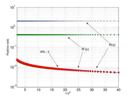
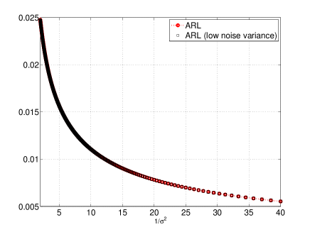
In this simulation part, we have considered an array constituted by $L=10$ sensors. The sources are chosen to be close where $\theta_{FF}=\pi/3$ and $\theta_{NF}=\pi/3.1$ and the range of this source belongs to the interval $[0.62(d^{3}(L-1)^{3}/T)\lambda,2d^{2}(L-1)^{2}/\lambda]$ [5] where $d=0.0125$ m and the carrier frequency is $f_{0}=10$ Mhz (the wavelength is $\lambda=c/f_{0}$ where $c$ is celerity of the light). The modulus of the NF sources is fixed to ten times higher than the modulus of FF source. It is normal to assume that the source which is the closest has a higher power than the one which belongs to the FF. The number of snapshot is $T=100$. On Fig. 1, we have reported the positive roots of each polynomials $R(x)$, $R^{\prime}(x)$ and the analytic ARL given in expression (28). As we can see one root for polynomials $R(x)$ and $R^{\prime}(x)$ are independent from the noise variance. These two roots have to be ignored. In addition, we can see that the one root for $R(x)$ and $R^{\prime}(x)$ are equal and follow a decreasing function w.r.t. the inverse of the noise variance. Moreover, the analytic ARL given in expression (28) is in good agreement with these roots and thus assess the validity of the derivations given in the previous section. The ARL given in expression (28) and the approximated ARL under the assumption of low noise variance given in expression (30) are reported on Fig. 2. It is important to highlight the good accuracy of the proposed approximated ARL.

Figure 1: (a) Positive roots for polynomials $R(x)$, $R^{\prime}(x)$ and analytic ARL given in expression (28) vs. the inverse of the noise variance. (b) ARL given in expression (28) and the approximated ARL under the assumption of low noise variance given in expression (30) vs. the inverse of the noise variance.

5 Conclusion

In this paper, we have derived and analyzed the Angular Resolution Limit (ARL) based on the resolution of the linearized Smith’s equation for the new and realistic scenario where far-field and near-field sources are mixed. Generally speaking, the ARL is important and fundamental since this quantity gives the limit in the resolvability/separation of two closely spaced signals in term of their direction of arrivals. We show that for the chosen application, the resolution of the Smith’s equation turns to be the selection of the ”right” root of a 4-th order polynomial. This allows us to give a closed-form (analytic) expression of the ARL.

6 References

References

• [1] H. Krim and M. Viberg, ”Two decades of array signal processing research: the parametric approach”, IEEE Signal Processing Magazine, Volume 13, Issue 4, July 1996.
• [2] J. Liang and D. Liu, ”Passive Localization of Mixed Near-Field and Far-Field Sources Using Two-stage MUSIC Algorithm”, IEEE Trans. Signal Process., Volume: 58 Issue: 1, Jan. 2010, pp: 108 - 120
• [3] P. Stoica and R.L. Moses, Spectral Analysis of Signals, Prentice Hall, 2005.
• [4] Y. D. Huang and M. Barkat, ”Near-field multiple source localization by passive sensor array”, IEEE Trans. Antennas Propag., vol. 39, no. 7, pp. 968-975, Jul. 1991.
• [5] E. Grosicki, K. Abed-Meraim, and Y. Hua, ”A weighted linear prediction method for near-field source localization”, IEEE Trans. Signal Process., vol. 53, pp. 3651- 3660, Oct. 2005.
• [6] S. T. Smith, ”Statistical resolution limits and the complexified Cramer-Rao bound”, IEEE Trans. Signal Process., vol. 53, pp. 1597-1609, May 2005.
• [7] M. N. El Korso, R. Boyer, A. Renaux and S. Marcos, ” Statistical resolution limit for the multidimensional harmonic retrieval model: Hypothesis test and Cramer-Rao bound approaches”, EURASIP Journal on Advances in Signal Processing, special issue ”Advances in Angle-of-Arrival and Multidimensional Signal Processing for Localization and Communications”, no. 12, pp. 1 14, 2011.
• [8] R. Boyer, ”Performance bounds and angular resolution limit for the moving co-located MIMO radar”, IEEE Trans. Signal Process., vol. 59, no. 4, pp. 1539 1552, 2011.
• [9] M. N. El Korso, R. Boyer, A. Renaux and S. Marcos, ”Statistical resolution limit of the uniform linear cocentered orthogonal loop and dipole array”, IEEE Trans. Signal Process., Volume: 59, Issue: 1, Jan. 2011, pp. 425-431.