Electron-hole symmetry and solutions of Richardson pairing model

Abstract

Richardson approach provides an exact solution of the pairing Hamiltonian. This Hamiltonian is characterized by the electron-hole pairing symmetry, which is however hidden in Richardson equations. By analyzing this symmetry and using an additional conjecture, fulfilled in solvable limits, we suggest a simple expression of the ground state energy for an equally-spaced energy-level model, which is applicable along the whole crossover from the superconducting state to the pairing fluctuation regime. Solving Richardson equations numerically, we demonstrate a good accuracy of our expression.

March 18, 2024

I Introduction

As shown by Richardson, the “reduced” Hamiltonian of the Bardeen-Cooper-Schrieffer (BCS) theory of superconductivity is exactly solvableRich1 . The Richardson approach is based on the canonical ensemble, i.e., the number of particles is fixed, while the BCS theory corresponds to the grand canonical description, which becomes accurate in the large-sample limit. In addition, the BCS theory provides only a mean-field approximation, which nevertheless turns out to be exactRich3 in the large-sample limit due to peculiarities of the “reduced” BCS potential. However, the grand canonical BCS theory is definitely not applicable for small-sized systems accommodating few pairs only. Significant improvements, nevertheless, are possible if one incorporates canonical approach into the BCS model (particle-number projected BCS), but still a rather heavy numerics is needed to proceed with computationsBraun . For the applicability of the canonical ensemble to the theory of superconductivity see Ref. Bogoliubov1 .

In contrast to the BCS theory, the Richardson method yields an exact solution to the many-body problem involving BCS pairing Hamiltonian. Within this approach, the energy of the system of $N$ correlated pairs is expressed through the sum of $N$ energy-like quantities, which satisfy the system of $N$ coupled nonlinear equations, called Richardson equations. It is remarkable that they are also derivable through the algebraic Bethe-ansatz approachPogosyan , so that the Richardson equations can be considered as one of the examples of Bethe-ansatz equations. However, it turns out that solving the Richardson equations is a formidable task. Up to now, they have been evaluated explicitly only in few special cases. In particular, no analytical solution exists for the crossover between the superconducting state and the pairing fluctuation regime, which is relevant for small-sized systems even for zero temperature. In this situation, no small parameter seems to exist, which could be used to construct some expansion. For this case, the Richardson equations are tackled numerically, when studying small systems described by pairing Hamiltonian, among which are nanosized superconducting grains Dukel , nuclei Dukel1 , ultracold atoms Belzig , bubbles in liquid helium Gladilin1 (for studies of correlation functions, see Ref. Osterloh ).

The aim of the present paper is to apply symmetry arguments in order to provide analytical results for the crossover region. It is actually well known that symmetry considerations can be very helpful in situations, when brute-force methods are not so efficient. We show that the BCS pairing Hamiltonian has an electron-hole (e-h) symmetry and we then try to reveal the impact of this symmetry for the ground state energy for the arbitrary number of pairs and interaction constant. The case of the equally-spaced model is considered, when the energy levels of noninteracting particles are distributed equidistantly. The impact of e-h symmetry can be most readily revealed in this particular case.

Although the e-h symmetry is encoded in the pairing Hamiltonian, it does not show up explicitly in Richardson equations. From the symmetry arguments, we suggest a simple explicit formula for the ground state energy, which constitutes a main result of this paper. Within our approach, we use a conjecture on the $N$-dependence of the dominant contribution to the ground state energy (when all other parameters are fixed). This hypothesis is justified by the fact that a guessed simple dependence on $N$ emerges in very different analytically-solvable limits. Under this assumption, we actually reduce the problem to the resolution of a single Richardson equation, which is far simpler than the solution of the full set of equations. The resulting expression for the ground state energy is also in a perfect agreement with known results in these limits, although we do not solve the whole system of Richardson equations. In order to address the accuracy of our formula in the crossover regime, we solve numerically the full system of these equations for $N$ pairs changing from $N=1$ to 50 and compare the results. We found a very good accuracy for systems with small number of pairs, which are of particular interest due to limitations of BCS treatment in this case. For systems with larger number of pairs, the maximum error, which corresponds to the regime of intermediate strength of coupling, grows. Nevertheless, our expression remains applicable in this case too. Our approach can be useful for other types of Bethe-ansatz equations, especially for those, which correspond to Gaudin-like models.

Though BCS Hamiltonian is rather simple, its applicability to small diffusive superconducting grains has been proved, see, e.g., Refs. Kurland ; Aleiner ; Ralph . The crucial condition is that the Thouless energy, which gives the inverse time to diffuse across the grain Vinokur , must be much larger than the average energy level spacingKurland . Also important is to have the Thouless energy much larger than the superconducting gap (see Appendix B of Ref. Aleiner ). It is less obvious what should be a relation between the energy level spacing and the superconducting gap. In particular, it was argued in Ref. Ralph (see also Ref. Aleiner ) that the BCS Hamiltonian probably can be considered as a toy model only, when the gap becomes much smaller than the level spacing.

II Model

We consider a system of fermions of two sorts, for instance, with spins up and down. Particles attract each other through the BCS “reduced” potential, coupling only fermions of different sorts and with zero total momenta as

$$\mathcal{V}=-V\sum_{\mathbf{k},\mathbf{k}^{\prime}}a_{\mathbf{k}^{\prime}\uparrow}^{\dagger}a_{-\mathbf{k}^{\prime}\downarrow}^{\dagger}a_{-\mathbf{k}\downarrow}a_{\mathbf{k}\uparrow}.$$ (1)

The total Hamiltonian is $H=H_{0}+\mathcal{V}$, where

$$H_{0}=\sum_{\mathbf{k}}\varepsilon_{\mathbf{k}}\left(a_{\mathbf{k}\uparrow}^{\dagger}a_{\mathbf{k}\uparrow}+a_{\mathbf{k}\downarrow}^{\dagger}a_{\mathbf{k}\downarrow}\right).$$ (2)

The summation in the right-hand side (RHS) of Eq. (1) runs only over the states with kinetic energies $\varepsilon_{\mathbf{k}}$ and $\varepsilon_{\mathbf{k}^{\prime}}$ located in the energy band between $\varepsilon_{F_{0}}$ and  $\varepsilon_{F_{0}}+\Omega$ (Debye window). These energies are distributed equidistantly (equally-spaced model), so that the difference between two nearest values of $\varepsilon_{\mathbf{k}}$ is $1/\rho$. The density of states $\rho$ increases with the system volume, while the interaction constant $V$ decreases, so that the dimensionless interaction constant $v=\rho V$ in superconductors is finite and, in the large-sample limit, it can be treated as a material characteristics. In the BCS theory, the energy interval between $\varepsilon_{F_{0}}$ and  $\varepsilon_{F_{0}}+\Omega$ is assumed to be always half-filled, while $\Omega/2$ is the Debye frequency. Thus, the total number of available states with up or down spins in the Debye window is $N_{\Omega}\equiv\rho\Omega$, while $N=N_{\Omega}/2$; $\varepsilon_{\mathbf{k}}$ runs from $\varepsilon_{F_{0}}$ to $\varepsilon_{F_{0}}+(N_{\Omega}-1)/\rho$ taking $N_{\Omega}$ values in total.

While it is supposed that the half-filling configuration only is physically meaningful, one can consider other fillings and at least treat the problem from the purely mathematical perspective. Note however that it was argued in Ref. Geyer that such a model might be relevant to some semiconductors (see also Ref. Eagles ). Introduction of the extra degree of freedom, which is a filling, is an important ingredient of our analysis. By considering the energy of the system formally as a function of $N$ (with all other input parameters fixed), we are going to obtain a valuable information on the half-filling situation. Numerical results will be presented for $N=N_{\Omega}/2$ only. For the sake of simplicity, we will focus on even values of $N_{\Omega}$.

In the present paper, we concentrate on the equally-spaced model, which provides a simplest but physically meaningful distribution of energy levels. Therefore, this model is the most attractive starting point to study the impact of e-h symmetry on the solutions of Richardson model. Superconducting correlations were also studied in finite-size system with random spacings of levels, distributed in accordance with the gaussian orthogonal ensemble, using mean-fieldAmbeg and exact Richardson approachesDussel . Such a statistics is typical for small metallic grainsGorkov . It was shown Dussel that the crossover between the superconducting state and the fluctuation-dominated regime is smooth, similarly to the case of the equally-spaced model.

The Hamiltonian, defined in Eqs. (1) and (2), is exactly solvableRich1 . The energy of $N$ pairs is given by the sum of $N$ rapidities $R_{j}$ ($j=1$,…, $N$) as $E_{N}=\sum_{j}R_{j}$. The Richardson equation for each rapidity $R_{j}$ reads

$$1=\sum_{\mathbf{k}}\frac{V}{2\varepsilon_{\mathbf{k}}-R_{j}}+\sum_{l,l\neq j}\frac{2V}{R_{j}-R_{l}},$$ (3)

where the summation in the first term is performed over $\varepsilon_{\mathbf{k}}$ located in the Debye window. Note that the dependence of $E_{N}$ on $N$ thus enters through the number of equations.

III The electron-hole symmetry

Now we discuss the internal electron-hole symmetry contained in the Hamiltonian, from which we are going to deduce an information on the solutions of Richardson equations. Let us introduce creation operators for holes as $b_{\mathbf{k}\uparrow}^{\dagger}=a_{\mathbf{k}\uparrow}$ and $b_{\mathbf{k}\downarrow}^{\dagger}=a_{\mathbf{k}\downarrow}$. By using commutation relations for fermionic operators, it is easy to rewrite the Hamiltonian in terms of holes as

$$H=-VN_{\Omega}+ 2 \sum_{\mathbf{k}}\varepsilon_{\mathbf{k}}-\sum_{\mathbf{k}}\left(\varepsilon_{\mathbf{k}}-V\right)\left(b_{\mathbf{k}\uparrow}^{\dagger}b_{\mathbf{k}\uparrow}+b_{\mathbf{k}\downarrow}^{\dagger}b_{\mathbf{k}\downarrow}\right)$$

$$- V \sum_{\mathbf{k},\mathbf{k}^{\prime}}b_{\mathbf{k}^{\prime}\uparrow}^{\dagger}b_{-\mathbf{k}^{\prime}\downarrow}^{\dagger}b_{-\mathbf{k}\downarrow}b_{\mathbf{k}\uparrow}.$$ (4)

The first two terms of the RHS of Eq. (4) are numbers. They give the potential energy and the kinetic energy of the Debye window completely filled by electron pairs, respectively. The fourth term coincides precisely with the interaction potential in terms of electrons, given by Eq. (1). To analyze the third term, we introduce $\xi_{\mathbf{k}}^{{}^{\prime}}$, defined as $\xi_{\mathbf{k}}^{{}^{\prime}}=$ $\varepsilon_{F_{0}}+(N_{\Omega}-1)/\rho-\varepsilon_{\mathbf{k}}$, which takes values $0$, $1/\rho$, $2/\rho$, …, $(N_{\Omega}-1)/\rho$, so that $\xi_{\mathbf{k}}^{{}^{\prime}}$ runs over all the states starting from the top of the Debye window towards its bottom, i.e., in the inverse order. Then, $-(\varepsilon_{\mathbf{k}}-V$) can be represented as $\xi_{\mathbf{k}}^{{}^{\prime}}+(V-\varepsilon_{F_{0}}-(N_{\Omega}-1)/\rho)$. A similar term in the Hamiltonian for electrons, given by Eq. (2), contains a factor $\xi_{\mathbf{k}}+\varepsilon_{F_{0}}$, where $\xi_{\mathbf{k}}$ takes values $0$, $1/\rho$, $2/\rho$, …, $(N_{\Omega}-1)/\rho$, so that it runs over all states starting from the bottom to the top of the same energy band.

Thus, due to peculiarities of the interaction potential, there exists a symmetry between electron and hole pairs in the Hamiltonian. Moreover, due to the equally-spaced distribution of energy levels in the Debye window, the ground state energy of $N$ electron pairs can be explicitly expressed through the energy of $N_{\Omega}-N$ electron pairs, with $\varepsilon_{F_{0}}$ changed into $(V-\varepsilon_{F_{0}}-(N_{\Omega}-1)/\rho)$. We therefore treat this energy $E_{N}(\varepsilon_{F_{0}})$ as a function of $\varepsilon_{F_{0}}$, which is an arbitrary nonzero number, and a discrete variable $N$, which runs over the set $1,2,...,N_{\Omega}$. Since the bare kinetic energy of a filled Debye window is given by the sum of terms of the arithmetic progression, $2N_{\Omega}\varepsilon_{F_{0}}+N_{\Omega}(N_{\Omega}-1)/\rho$, we arrive at the identity

$$E_{N}(\varepsilon_{F_{0}})=E_{N_{\Omega}-N}\left(V-\varepsilon_{F_{0}}-\frac{N_{\Omega}-1}{\rho}\right)$$

$$-VN_{\Omega}+2N_{\Omega}\varepsilon_{F_{0}}+\frac{N_{\Omega}(N_{\Omega}-1)}{\rho}.$$ (5)

Note that in the case of more complex types of energy-level distributions in the conduction band, one has also to change the distribution, when switching from electron pairs to hole pairs, which corresponds to counting levels from the top instead of counting them from the bottom of the Debye window. This makes the situation more subtle compared to the equally-spaced model. Nevertheless, the duality between the electrons and holes still exists, since this feature is a direct consequence of BCS interaction potential, so that Eq. (4) stays valid.

Next, we split $E_{N}(\varepsilon_{F_{0}})$ into the additive contribution $2N\varepsilon_{F_{0}}$, which simply corresponds to the shift of all rapidities, and $E_{N}^{{}^{\prime}}$, the latter being independent of $\varepsilon_{F_{0}}$

$$E_{N}(\varepsilon_{F_{0}})=2N\varepsilon_{F_{0}}+E_{N}^{{}^{\prime}}.$$ (6)

By substituting Eq. (6) to (5), we arrive at the functional equation

$$E_{N}^{{}^{\prime}}=E_{N_{\Omega}-N}^{{}^{\prime}}+(N_{\Omega}-2N)\left(V-\frac{N_{\Omega}-1}{\rho}\right),$$ (7)

which is still exact. This remarkable condition will enable us to relate the condensation energy of $N$ pairs to the condensation energy of $N_{\Omega}-N$ pairs. Note that it is automatically fulfilled for the half-filling, $N=N_{\Omega}/2$.

We would like to stress that, although the e-h symmetry can be rather easily extracted from the Hamiltonian, it is not obvious that the solution of $N$ equations is related to that of $N_{\Omega}-N$ equations through such a simple and universal relation as Eq. (7). For the moment, we do not know how this relation can be derived directly from Richardson equations.

Since $E_{N}^{{}^{\prime}}$ is a function of the discrete variable $N$, which runs over $N_{\Omega}$ values, it can always be represented as a polynomial of $N$ of power $N_{\Omega}$. Alternatively, instead of expanding in elementary monomials $N^{n}$, one may use Pochhammer symbols defined as

$$(N)_{n}=N(N-1)...(N-n+1),$$ (8)

while $(N)_{0}\equiv 1$; so that $(N)_{n}$ may be treated as a polynomial of $N$ of power $n$. Then,

$$E_{N}^{{}^{\prime}}=\sum_{n=1}^{N_{\Omega}}e_{n}(N)_{n},$$ (9)

where $e_{n}$ is a set of unknown numbers.

Actually, $E_{N}^{{}^{\prime}}$ can be also split into the condensation energy $E_{N}^{(cond)}$ and the contribution coming from the bare kinetic energy. The latter is given universally by $N(N-1)/\rho$, which can be obviously described by the second term in the RHS of Eq. (9).

Up to now, all the results were exact. At this step, we make a conjecture that a dominant contribution to $E_{N}^{{}^{\prime}}$ is due to the first two terms in the sum of the RHS of Eq. (9) that is

$$E_{N}^{{}^{\prime}}\simeq e_{1}N+e_{2}N(N-1).$$ (10)

This assumption is fully reasonable, since such a form of $E_{N}^{{}^{\prime}}$ does emerge in three important limits, which are solvable analytically. Let’s discuss the condensation energy in these three limits, since the contribution from the kinetic energy, $N(N-1)/\rho$, is always in agreement with Eq. (10), as discussed above. The first limit is a regime of the very weak coupling realized for finite $N_{\Omega}$ ($v\ll 1/\ln(N_{\Omega})$), for which all the rapidities are located in real axis and approach the energy levels of noninteracting electrons. In this case, $E_{N}^{(cond)}=-VN$, so that Eq. (10) is satisfied. Another limit is the strong-coupling regime ($v\gg 1$), when all the rapidities are located far away from the line of one-electron levels in the complex plane. In this case, $E_{N}^{(cond)}$ containsRich1 terms proportional to $N$ and $N(N-1)$. At last, there is a limit of infinite $N$ at finite nonzero $v$; here also $E_{N}^{(cond)}$ has a similar formRich3 ; We . These three limits are quite different from each otherDussel ; Schechter ; Altshuler . It is actually the reason why we conjecture that the structure of the solution, given by Eq. (10), must remain robust in the intermediate region, which is characterized by finite $N_{\Omega}$ and arbitrary $v$.

Now we consider $e_{1}$ and $e_{2}$ as unknown numbers and substitute Eq. (10) into Eq. (7). We then equate coefficients of $(N)_{0}$, $(N)_{1}$ and $(N)_{2}$ in both sides of this equation and obtain a system of three linear equations for $e_{1}$ and $e_{2}$. These three equations turn out to be dependent, so they yield only a single condition as

$$e_{2}=-\frac{e_{1}}{N_{\Omega}-1}+\left(\frac{N_{\Omega}-1}{\rho}-V\right)\frac{1}{N_{\Omega}-1}.$$ (11)

At this stage, we are left with only one unknown number, $e_{1}$. It can be easily determined by considering a one-pair problem (as a “boundary condition” in the space of discrete $N$). In this case, $E_{1}^{{}^{\prime}}=e_{1}$, while $e_{1}$ is given by the solution of the single Richardson equation

$$V=\sum_{n=0}^{N_{\Omega}-1}\frac{1}{2n/\rho-e_{1}},$$ (12)

under the condition $e_{1}<0$, which ensures that we select the lowest-energy solution; then, $-e_{1}$ is a binding energy of a single pair. In the general case, $e_{1}$ has to be determined numerically, while exact analytical results are available in certain limits, as discussed below. Note that Eq. (12) can be rewritten in terms of $\Gamma$-functions.

The expression of $E_{N}^{{}^{\prime}}$ is obtained by substituting Eq. (11) to Eq. (10) as

$$E_{N}^{{}^{\prime}}=\frac{N(N-1)}{\rho}+Ne_{1}\left(1-\frac{N-1}{N_{\Omega}-1}\right)-VN\frac{N-1}{N_{\Omega}-1},$$ (13)

where the first term comes from the bare kinetic energy, while two others give the condensation energy. It is remarkable that our method reproduces the first contribution automatically in the exact form. The condensation energy per pair then reads

$$E_{N}^{(cond)}/N=e_{1}\left(1-\frac{N-1}{N_{\Omega}-1}\right)-V\frac{N-1}{N_{\Omega}-1}.$$ (14)

Eq. (14) supplemented by Eq. (12) is the main result of this paper.

IV Discussion

Let us now consider the limits when Eq. (12) can be solved analytically, in order to see whether Eq. (14) gives reasonable results.

We start with the limit of the very weak coupling, in which the solution of Eq. (12) approaches the lowest level so closely that the mutual separation becomes much smaller than $1/\rho$ and, moreover, contributions from other levels can be neglected. Then, we obtain a simple solution $e_{1}=-V$. By estimating dropped contributions due to other levels, we obtain a criterion of applicability of this result as $v\ll 1/\ln(N_{\Omega})$. In this case, $E_{N}^{(cond)}/N$ reduces to $-V$, as it must be, due to the cancellation in the RHS of Eq. (14). Note that the condensation energy per pair in this limit is independent of filling.

Next, we consider an opposite limit, when the separation between the single rapidity and the lowest level is much larger than $1/\rho$ and the number of levels $N_{\Omega}$ is also large. This enables us to replace the sum in the RHS of Eq. (12) by the integral, which gives

$$e_{1}\simeq-2\Omega\frac{\exp(-2/v)}{1-\exp(-2/v)}.$$ (15)

The condition of applicability of this result is thus twofold: $N_{\Omega}\gg 1$ and $N_{\Omega}\exp(-2/v)/(1-\exp(-2/v))\gg 1$. The infinite-sample limit, when $v$ is fixed and finite, thus always satisfies these criteria. It is also easy to see that $\mid e_{1}\mid$ given by Eq. (12) is much larger than $V$ in the large-sample limit, $N_{\Omega}\longrightarrow\infty$, so that $V\sim\mid e_{1}\mid/N_{\Omega}$. This means that in this limit $V$ can be neglected in Eq. (14). Then,

$$E_{N}^{(cond)}/N\simeq-2\left(\Omega-\frac{N}{\rho}\right)\frac{\exp(-2/v)}{1-\exp(-2/v)},$$ (16)

which, for the half-filling, coincides with the BCS expression for the condensation energy per $N$ (and with Richardson large-$N$ result for the same fillingRich3 ). For arbitrary filling, it also coincides with the results of both the mean-field treatment and of the Richardson approachWe .

We would like to stress that the obtained results are highly nontrivial. Indeed, the condensation energy given by Eq. (14) consists of two terms. In the limit of a very weak coupling, both of them are of the same order, while their combination gives the exact result within all numerical prefactors. In contrast, in the large-sample limit $N_{\Omega}\longrightarrow\infty$, when interaction constant $v$ is finite and nonzero, one of the terms becomes of the order of $1/N_{\Omega}$ compared to another one, so that it can be dropped as an underextensive contribution, while the remaining term again gives a correct result within all numerical prefactors. Such a very subtle interplay between the two terms indicates that the suggested formula for the condensation energy must remain accurate not only in the considered limits.

Actually, by manipulating the single-pair binding energy, which must be determined numerically, we circumvent the problem of inapplicability of large-$N$ approaches to the normal state, pointed out by Richardson in Ref. Rich3 . This difficulty can be traced back to the non-analytic dependence of condensation energy on $V$ in this limit, while in the limit of a very weak interaction it is simply proportional to $V$. Moreover, in the first case, this energy is an extensive quantity, while in the second one, it becomes intensive. It is therefore challenging to unify both regimes within a single self-consistent formalism.

In order to explore the applicability range of the obtained expression of the condensation energy, we perform a systematic numerical solution of the full set of Richardson equations, as given by Eq. (3), for various values of $N$ from 1 to 50 and $v$ at the half-filling. Then, we compare the obtained numerical results with the prediction of Eq. (14) (where $e_{1}$ is obtained from the numerical solution of Eq. (12)). We also calculate the condensation energy by using the standard grand-canonical BCS theory. The only difference with the common version of this theory is the fact that we do not replace sums by integrals when solving the gap equation and also when calculating the condensation energy itself, which is of importance for systems with relatively small number of pairs, since these replacements are responsible for additional inaccuracies.

In the general case, the Richardson equations can be numerically solved by Newton-Raphson method with a good initial guess. An exact solution $R_{j}=2\varepsilon_{F_{0}}+2j/\rho\ (n=0,1,..,N-1)$ is a solution for $v=0$. Therefore, we start with such initial values and then find solutions with increasing $v$. In order to avoid the singularity, new variables $\lambda_{+},\lambda_{-}$ are introducedNumer1 . When $v$ is close to the critical $v_{c}$, the Newton-Raphson result does not converge to the solution if it starts from the other side of the singularityNumer2 . Therefore, an extrapolation step is taken for the new $v$ (close to $v_{c}$), as proposed in Ref. Numer2 .

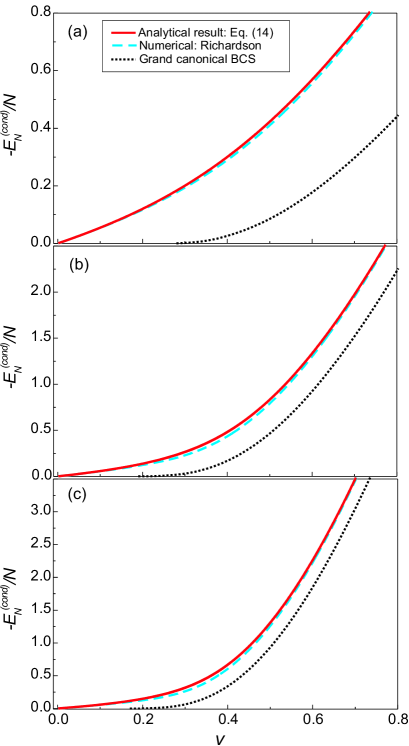
Figure 1: (Color online) The condensation energy per pair as a function of the interaction constant, for $N$ pairs: $N=5$ (a), $N=25$ (b), and $N=50$ (c). Red (gray) solid lines show the prediction according to our analytical formula (14), blue (light gray) dashed lines represent the results of the numerical solution of the full system of Richardson equations, black dotted lines correspond to the grand-canonical BCS result.

The results are presented in Fig. 1 for three particular values of $N$. The condensation energies are measured in terms of $2/\rho$. Fig. 1(a – c) give the dependence of the condensation energy per pair, as a function of $v$, for $N=5$, 25, and 50, respectively. Solid curves yield our prediction, dashed curves represent results of the numerical solution of the Richardson equations, and dotted lines are the grand-canonical BCS results. We see that there is generally a good agreement between the numerical results and those obtained from our formula. The similar agreement has been found for other values of $N$. Therefore, our conjecture is justified. In contrast, BCS results become accurate in the large-$N$ limit only: as it is known, there is a range of small $v$ for any $N$, when the grand-canonical BCS theory is qualitatively incorrect, since it predicts a disappearance of superconducting correlations (see Fig. 1). In this fluctuation-dominated regime, our approach works well. We found that the largest relative errors for the three cases illustrated in Fig. 1 are $3$, $15$, and $23$ percent, respectively. Thus, our approach is more efficient for small $N$, this case being more interesting due to limitations of BCS theory for systems with small number of pairs. We also would like to note that the accuracy can, in principle, be improved by considering more terms in Eq. (9) and using two-pairs ”boundary condition” (and possibly other configurations with even more pairs), although such a procedure would lack simple analytical results, in contrast to the present approach.

Within our approach, a single-pair binding energy $-e_{1}$ plays a very important role, although we deal with the many-pair system. It provides an energy scale, which is alternative to the superconducting gap $\Delta$. Interestingly, the existence of an additional scale for finite systems was revealed some time ago in Ref. Schechter , where it was shown that BCS results for the ground state energy become inadequate already for level spacings $1/\rho\approx 2\Delta^{2}/\Omega$, which are much smaller than $\Delta$ at $v\ll 1$. Let us point out that, as easily seen by a direct comparison, in the large-sample limit, $2\Delta^{2}/\Omega$ is nothing but $-e_{1}$ when $v$ is small. It is very unlikely that such a coincidence is accidental. Therefore, we believe that the additional energy scale found in Ref. Schechter is connected to the single-pair binding energy. Note that it was recently argued JETPLett that standard BCS results for the condensation energy in the thermodynamical limit can be also interpreted in a simple way through the single-pair binding energy and not through $\Delta$, as usual. In particular, in this limit, $-e_{1}$ and $\Delta$ have similar, but different dependencies on $v$, since $-e_{1}\sim\exp(-2/v)$, while $\Delta\sim\exp(-1/v)$ at $v\ll 1$, as discussed in detail in Ref. JETPLett .

It is perspective to extend our analysis to excited states. We also think that, probably, similar ideas can be applied to other types of energy-level distributions, in particular, to those, which are characterized by the inversion symmetry around the middle point of the band. Furthermore, the analysis of the electron-hole symmetries can be helpful in treatments of other Bethe-ansatz equations, among which Richardson equations are just one of the examples.

Notice that the derived exact relation for the condensation energy, given by Eq. (7), can be used as a test to check the accuracy of the numerically-found solutions of Richardson equations.

V Conclusions

We suggested a simple expression for the ground state energy of the pairing Hamiltonian for the case of the equally-spaced model along the crossover from the superconducting regime to the pairing fluctuation regime. This expression is derived from the peculiar electron-hole symmetry of the pairing Hamiltonian and relies on the conjecture, which enables us to reduce the task to the one-pair problem. The electron-hole symmetry is encoded in the Hamiltonian, but it is hidden in Richardson equations, which provide an exact many-body solution of the problem. The obtained expression of the ground state energy depends on the binding energy of a single pair, which, in the general case, must be determined numerically by solving a single Richardson equation. The latter problem is much simpler than the solution of the full set of Richardson equations. This quantity also provides an additional energy scale associated with superconducting correlations, which seems to be connected with the energy scale revealed in Ref. Schechter .

The comparison with the results of the full numerical resolution of Richardson equations demonstrated a generally good accuracy of the suggested formula, while the usual grand-canonical BCS approach fails even qualitatively in the fluctuation-dominated regime. The accuracy is better in the case of the system with small number of pairs, which is of particular interest due to limitations of BCS method in this situation.

- (1) R. W. Richardson, Phys. Lett. 3 (1963) 277.
- (2) R. W. Richardson, J. Math. Phys. 18 (1977) 1802; M. Gaudin, J. Phys. (Paris) 37 (1976) 1087.
- (3) K. Dietrich, H. J. Mang, and J. H. Pradal, Phys. Rev. B 22 (1964) 135; F. Braun and J. von Delft, Phys. Rev. Lett. 81 (1998) 4712.
- (4) N. N. Bogoliubov, Usp. Fiz. Nauk 67 (1959) (549) [Sov. Phys. Usp. 2 (1959) 236].
- (5) J. von Delft and R. Poghossian, Phys. Rev. B 66 (2002) 134502.
- (6) J. Dukelsky, S. Pittel, and G. Sierra, Rev. Mod. Phys. 76 (2004) 643.
- (7) N. Sandulescu, B. Errea, and J. Dukelsky, Phys. Rev. C 80 (2009) 044335.
- (8) S. Staudenmayer, W. Belzig, and C. Bruder, Phys. Rev. A 77 (2008) 013612.
- (9) J. Tempere, V. N. Gladilin, I. F. Silvera, and J. T. Devreese, Phys. Rev. B 72 (2005) 094506.
- (10) L. Amico and A. Osterloh, Phys. Rev. Lett. 88 (2002) 127003; H.-Q. Zhou, J. Links, R. H. McKenzie, and M. D. Gould, Phys. Rev. B 56 (2002) 060502(R); G. Gorohovsky and E. Bettelheim, Phys. Rev. B 84 (2011) 224503.
- (11) I. L. Kurland, I. L. Aleiner, and B. L. Altshuler, Phys. Rev. B 62 (2000) 14886.
- (12) I. L. Aleiner, P. W. Brouwer, and L. I. Glazman, Phys. Rep. 358 (2002) 309.
- (13) J. von Delft and D. C. Ralph, Phys. Rep. 345 (2001) 61.
- (14) I. S. Beloborodov, A. V. Lopatin, V. M. Vinokur, and K. B. Efetov, Rev. Mod. Phys. 79 (2007) 469.
- (15) I. Snyman and H. B. Geyer, Phys. Rev. B 73 (2006) 144516.
- (16) D. M. Eagles, Phys. Rev. 186 (1969) 456.
- (17) R. A. Smith and V. Ambegaokar, Phys. Rev. Lett. 77 (1996) 4962.
- (18) G. Sierra, J. Dukelsky, G. G. Dussel, J. von Delft, and F. Braun, Phys. Rev. B 61 (2000) R11890.
- (19) L. P. Gor kov and G. M. Eliashberg, Zh. Eksp. Theor. Fiz. 48 (1965) 1407 [Sov. Phys. JETP 21 (1965) 940]; K. B. Efetov, Adv. Phys. 32 (1983) 53.
- (20) M. Crouzeix and M. Combescot, Phys. Rev. Lett. 107 (2011) 267001; W. V. Pogosov, J. Phys.: Condens. Matter 24 (2012) 075701.
- (21) M. Schechter, Y. Imry, Y. Levinson, and J. von Delft, Phys. Rev. B 63 (2001) 214518.
- (22) E. A. Yuzbashyan, A. A. Baytin, and B. L. Altshuler, Phys. Rev. B 71 (2005) 094505.
- (23) A. Faribault, P. Calabrese, and J. S. Caux, J. Math. Phys. 50 (2009) 095212.
- (24) S. Rombouts, D. Van Neck, and J. Dukelsky, Phys. Rev. C 69 (2004) 061303(R).
- (25) W. V. Pogosov and M. Combescot, Pis’ma v ZhETF 92 (2010) 534 [JETP Lett. 92 (2010) 534].