$4$-Regular oriented graphs with
optimum skew energy

Abstract

Let $G$ be a simple undirected graph, and $G^{\sigma}$ be an oriented graph of $G$ with the orientation $\sigma$ and skew-adjacency matrix $S(G^{\sigma})$. The skew energy of the oriented graph $G^{\sigma}$, denoted by $\mathcal{E}_{S}(G^{\sigma})$, is defined as the sum of the absolute values of all the eigenvalues of $S(G^{\sigma})$. In this paper, we characterize the underlying graphs of all $4$-regular oriented graphs with optimum skew energy and give orientations of these underlying graphs such that the skew energy of the resultant oriented graphs indeed attain optimum. It should be pointed out that there are infinitely many 4-regular connected optimum skew energy oriented graphs, while the $3$-regular case only has two graphs: $K_{4}$ the complete graph on $4$ vertices and $Q_{3}$ the hypercube.

Keywords: oriented graph, skew energy, skew-adjacency matrix, regular graph

AMS Subject Classification Numbers: 05C20, 05C50, 05C90

1 Introduction

Let $G$ be a simple undirected graph with vertex set $V(G)=\{v_{1},v_{2},\ldots,v_{n}\}$, and let $G^{\sigma}$ be an oriented graph of $G$ with the orientation $\sigma$, which assigns to each edge of $G$ a direction so that the induced graph $G^{\sigma}$ becomes an oriented graph or a directed graph. Then $G$ is called the underlying graph of $G^{\sigma}$. The skew-adjacency matrix of $G^{\sigma}$ is the $n\times n$ matrix $S(G^{\sigma})=[s_{ij}]$, where $s_{ij}=1$ and $s_{ji}=-1$ if $\langle v_{i},v_{j}\rangle$ is an arc of $G^{\sigma}$, otherwise $s_{ij}=s_{ji}=0$. The skew energy [1] of $G^{\sigma}$, denoted by $\mathcal{E}_{S}(G^{\sigma})$, is defined as the sum of the absolute values of all the eigenvalues of $S(G^{\sigma})$. Obviously, $S(G^{\sigma})$ is a skew-symmetric matrix, and thus all the eigenvalues are purely imaginary numbers.

In theoretical chemistry, the energy of a given molecular graph is related to the total $\pi$-electron energy of the molecule represented by that graph. Consequently, the graph energy has some specific chemistry interests and has been extensively studied, since the concept of the energy of simple undirected graphs was introduced by Gutman in [4]. We refer the survey [5] and the book [8] to the reader for details. Up to now, there are various generalizations of the graph energy, such as the Laplacian energy, signless Laplacian energy, incidence energy, distance energy, and the Laplacian-energy like invariant for undirected graphs, and the skew energy and skew Laplacian energy for oriented graphs.

Adiga et al. [1] first defined the skew energy of an oriented graph, and investigated some properties of the skew energy. Then, Shader et al. [9] studied the relationship between the spectra of a graph $G$ and the skew-spectra of an oriented graph $G^{\sigma}$ of $G$, which would be helpful to the study of the relationship between the energy of $G$ and the skew energy of $G^{\sigma}$. Hou and Lei [6] characterized the coefficients of the characteristic polynomial of the skew-adjacency matrix of an oriented graph. Moreover, other bounds and extremal graphs of some classes of oriented graphs have been established. In [7] and [10], Hou et al. determined the oriented unicyclic graphs with minimal and maximal skew energy and the oriented bicyclic graphs with minimal and maximal shew energy, respectively. The skew energy of orientations of hypercubes were discussed by Tian [11]. Later, Gong and Xu [3] characterized the 3-regular oriented graphs with optimum skew energy. Recently, we [2] studied the skew energy of random oriented graphs.

Back to the paper Adiga et al. [1], where they derived a sharp upper bound for the skew energy of an oriented graph $G^{\sigma}$ in terms of the order $n$ and the maximum degree $\Delta$ of $G^{\sigma}$, that is,

$$\mathcal{E}_{S}(G)\leq n\sqrt{\Delta}\,.$$

They showed that the equality holds if and only if $S(G^{\sigma})^{T}S(G^{\sigma})=\Delta I_{n}$, which implies that $G^{\sigma}$ is $\Delta$-regular. In the following, we will call an oriented graph $G^{\sigma}$ on $n$ vertices with maximum degree $\Delta$ an optimum skew energy oriented graph if $\mathcal{E}_{S}(G^{\sigma})=n\sqrt{\Delta}$. A natural question is proposed in [1]:

Which $k$-regular graphs on $n$ vertices have orientations $G^{\sigma}$ with $\mathcal{E}_{S}(G^{\sigma})=n\sqrt{\Delta}$, or equivalently, $S(G^{\sigma})^{T}S(G^{\sigma})=\Delta I_{n}$ ?

In the same paper, they answer the question for $k=1$ and $k=2$. They showed that a $1$-regular graph on $n$ vertices has an orientation with $S(G^{\sigma})^{T}S(G^{\sigma})=I_{n}$ if and only if $n$ is even and it is $\frac{n}{2}$ copies of $K_{2}$; while a $2$-regular graph on $n$ vertices has an orientation with $S(G^{\sigma})^{T}S(G^{\sigma})=2I_{n}$ if and only if $n$ is a multiple of $4$ and it is a union of $\frac{n}{4}$ copies of $C_{4}$. Later, Gong and Xu [3] characterized all $3$-regular connected oriented graphs on $n$ vertices with $S(G^{\sigma})^{T}S(G^{\sigma})=3I_{n}$, which in fact are only two special graphs, the complete graph $K_{4}$ and the hypercube $Q_{3}$.

In this paper, we further consider the above question. We characterize all $4$-regular connected graphs $G$ that have oriented graphs $G^{\sigma}$ with $S(G^{\sigma})^{T}S(G^{\sigma})=4I_{n}$. It should be noted that the $4$-regular case is more complicated than the $3$-regular case, and in fact, there are infinitely many 4-regular connected optimum skew energy oriented graphs.

2 Preliminaries

In this section, we do some preparations with some notations and a few known results. Besides, we also get some intuitive conclusions that will be frequently used in the sequel of the paper.

Let $G=G(V,E)$ be a graph with vertex set $V$ and edge set $E$. For any $v\in V$, denote by $d_{G}(v)$ and $N_{G}(v)$ the degree and neighborhood of $v$ in $G$, respectively. For any subset $S\subseteq V$, $G[S]$ denotes the subgraph of $G$ induced by $S$. For a given orientation $\sigma$ of $G$, the resultant oriented graph is denoted by $G^{\sigma}=(V(G^{\sigma}),\Gamma(G^{\sigma}))$ and the skew-adjacency matrix of $G^{\sigma}$ by $S(G^{\sigma})$.

The following result is due to Adiga et al. [1].

Lemma 2.1

[1] Let $S(G^{\sigma})$ be the skew-adjacency matrix of an oriented graph $G^{\sigma}$. If $S(G^{\sigma})^{T}S(G^{\sigma})=kI$, then $|N(u)\cap N(v)|$ is even for any two distinct vertices $u$ and $v$ of $G^{\sigma}$.

Since our paper focuses on the investigation of $4$-regular graphs, the following result is more directly applied, which is in fact implied in Lemma 2.1.

Proposition 2.2

Let $G^{\sigma}$ be a $4$-regular oriented graph with skew-adjacency matrix $S(G^{\sigma})$. If $S(G^{\sigma})^{T}S(G^{\sigma})=4I$, then the underlying graph $G$ satisfies that $|N(u)\cap N(v)|\in\{0,2\}$ for any two adjacent vertices $u$ and $v$ and $|N(u)\cap N(v)|\in\{0,2,4\}$ for any two non-adjacent vertices $u$ and $v$.

Let $W=u_{1}u_{2}\cdots u_{k}$ (perhaps $u_{i}=u_{j}$ for $i\neq j$) be a walk from $u_{1}$ to $u_{k}$ and $\widehat{W}$ be the inverse walk of $W$ obtained from $W$ by replacing the ordering of vertices by its inverses, i.e., $\widehat{W}=u_{k}u_{k-1}\cdots u_{1}$. The sign of $W$ is defined as

$$\text{sgn}(W)=\prod_{i=1}^{k-1}s_{u_{i}u_{i+1}}.$$

It is easy to check that

$$\text{sgn}(\widehat{W})=\begin{cases}\text{sgn}(W)&\text{if\,\,}l(W)\text{\,\,is even},\\ -\text{sgn}(W)&\text{if\,\,}l(W)\text{\,\,is odd},\end{cases}$$

where $l(W)$ denotes the length of the walk $W$. Moreover, let $w_{uv}^{+}(k)$ and $w_{uv}^{-}(k)$ denote the number of all positive walks and negative walks starting from $u$ and ending at $v$ with length $k$, respectively.

Gong and Xu [3] obtained the following result on the relationship between the entries of $S^{k}$ and the number of walks between any pair of ordered vertices.

Lemma 2.3

[3] Let $S$ be the skew-adjacency matrix of an oriented graph $G^{\sigma}$ and $(u,v)$ be an arbitrary pair of ordered vertices of $G^{\sigma}$. Then

$$(S^{k})_{uv}=w_{uv}^{+}(k)-w_{uv}^{-}(k)$$

holds for any positive integer $k$.

For regular graphs, the following proposition is immediate.

Proposition 2.4

Let $G^{\sigma}$ be a $k$-regular oriented graph with skew-adjacency matrix $S$. Then $S^{T}S=kI$ if and only if for any two distinct vertices $u$ and $v$ of $G^{\sigma}$,

$$w_{uv}^{+}(2)=w_{uv}^{-}(2).$$

Throughout this paper, we just need to consider connected graphs and connected oriented graphs due to the following basic lemma. Recall that the union $G_{1}^{\sigma}\cup G_{2}^{\sigma}$ of two disjoint oriented graphs $G_{1}^{\sigma}=(V_{1},\Gamma_{1})$ and $G_{2}^{\sigma}=(V_{2},\Gamma_{2})$ is the oriented graph $G^{\sigma}=(V,\Gamma)$ where $V=V_{1}\cup V_{2}$ and $\Gamma=\Gamma_{1}\cup\Gamma_{2}$.

Lemma 2.5

[11] Let $G_{1}^{\sigma}$, $G_{2}^{\sigma}$ be two disjoint oriented graphs of order $n_{1}$, $n_{2}$ with skew-adjacency matrices $S(G_{1}^{\sigma})$, $S(G_{2}^{\sigma})$, respectively. Then for some positive integer $k$, $S(G_{1}^{\sigma})^{T}S(G_{1}^{\sigma})=kI_{n_{1}}$ and $S(G_{2}^{\sigma})^{T}S(G_{2}^{\sigma})=kI_{n_{2}}$ if and only if the skew-adjacency matrix $S(G_{1}^{\sigma}\cup G_{2}^{\sigma})$ of the union $G_{1}^{\sigma}\cup G_{2}^{\sigma}$ satisfies $S(G_{1}^{\sigma}\cup G_{2}^{\sigma})^{T}S(G_{1}^{\sigma}\cup G_{2}^{\sigma})=kI_{n_{1}+n_{2}}$.

We end this section by recursively defining two graph classes $\mathcal{G}_{i}$ and $\mathcal{H}_{j}$ for all positive integers $i$ and $j$, depicted in Figure 2.1 and Figure 2.2, respectively.

For the graph class $\mathcal{G}_{i}$, we define the initial graph $\mathcal{G}_{1}=(V(\mathcal{G}_{1}),E(\mathcal{G}_{1}))$, where

$$V(\mathcal{G}_{1})= \{u,v\}\cup\{u_{1},u_{2},v_{1},v_{2}\}\cup\{u_{3},u_{4},v_{3},v_{4}\},$$

$$E(\mathcal{G}_{1})= \{(u,u_{1}),(u,u_{2}),(u,v_{1}),(u,v_{2}),(v,u_{1}),(v,u_{2}),(v,v_{1}),(v,v_{2})\}$$

$$\cup\{(u_{1},u_{3}),(u_{1},u_{4}),(u_{2},u_{3}),(u_{2},u_{4}),(v_{1},v_{3}),(v_{1},v_{4}),(v_{2},v_{3}),(v_{2},v_{4})\}$$

$$\cup\{(u_{3},v_{4}),(v_{4},u_{4}),(u_{4},v_{3}),(v_{3},u_{3})\}.$$

Suppose that $\mathcal{G}_{i-1}$ is well defined. Below we will give the definition of $\mathcal{G}_{i}=(V(\mathcal{G}_{i}),E(\mathcal{G}_{i}))$.

$$V(\mathcal{G}_{i})= V(\mathcal{G}_{i-1})\cup\{u_{2i+1},u_{2j+2},v_{2i+1},v_{2i+2}\},$$

$$E(\mathcal{G}_{i})= E(\mathcal{G}_{i-1})\setminus\{(u_{2i-1},v_{2i}),(v_{2i},u_{2i}),(u_{2i},v_{2i-1}),(v_{2i-1},u_{2i-1})\}$$

$$\cup\{(u_{2i-1},u_{2i+1}),(u_{2i-1},u_{2i+2}),(u_{2i},u_{2i+1}),(u_{2i},u_{2i+2})\}$$

$$\cup\{(v_{2i-1},v_{2i+1}),(v_{2i-1},v_{2i+2}),(v_{2i},v_{2i+1}),(v_{2i},v_{2i+2})\}$$

$$\cup\{(u_{2i+1},v_{2i+2}),(v_{2i+2},u_{2i+2}),(u_{2i+2},v_{2i+1}),(v_{2i+1},u_{2i+1})\}.$$

Observe that $|V(\mathcal{G}_{i})|=4i+6$.

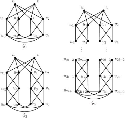
Figure 2.1: The graph class $\mathcal{G}_{i}$ for any positive integer $i$

For the other graph class $\mathcal{H}_{j}$, the initial graph $\mathcal{H}_{1}$ is defined as $\mathcal{H}_{1}=(V(\mathcal{H}_{1}),E(\mathcal{H}_{1}))$, where

$$V(\mathcal{H}_{1})= \{u,v\}\cup\{u_{1},u_{2},v_{1},v_{2}\}\cup\{u_{3},u_{4}\},$$

$$E(\mathcal{H}_{1})= \{(u,u_{1}),(u,u_{2}),(u,v_{1}),(u,v_{2}),(v,u_{1}),(v,u_{2}),(v,v_{1}),(v,v_{2})\}$$

$$\cup\{(u_{1},u_{3}),(u_{1},u_{4}),(u_{2},u_{3}),(u_{2},u_{4}),(v_{1},u_{3}),(v_{1},u_{4}),(v_{2},u_{3}),(v_{2},u_{4})\}.$$

Suppose now that we have given the definition of $\mathcal{H}_{j-1}$. Then $\mathcal{H}_{j}=(V(\mathcal{H}_{j}),E(\mathcal{H}_{j}))$ is defined as follows.

$$V(\mathcal{H}_{j})= V(\mathcal{H}_{j-1})\cup\{v_{2j-1},v_{2j},u_{2j+1},u_{2j+2}\},$$

$$E(\mathcal{H}_{j})= E(\mathcal{H}_{j-1})\setminus\{(v_{2j-3},u_{2j-1}),(v_{2j-3},u_{2j}),(v_{2j-2},u_{2j-1}),(v_{2j-2},u_{2j})\}$$

$$\cup\{(v_{2j-3},v_{2j-1}),(v_{2j-3},v_{2j}),(v_{2j-2},v_{2j-1}),(v_{2j-2},v_{2j})\}$$

$$\cup\{(u_{2j-1},u_{2j+1}),(u_{2j-1},u_{2j+2}),(u_{2j},u_{2j+1}),(u_{2j},u_{2j+2})\}$$

$$\cup\{(v_{2j-1},u_{2j+1}),(v_{2j-1},u_{2j+2}),(v_{2j},u_{2j+1}),(v_{2j},u_{2j+2})\}.$$

Obviously, $|V(\mathcal{H}_{j})|=4j+4$.

Figure 2.2: The graph class $\mathcal{H}_{j}$ for any positive integer $j$

3 Main results

In this section, we first characterize the underlying graphs of all $4$-regular oriented graphs with optimum skew energy. Then we give orientations of these underlying graphs such that the resultant oriented graphs have optimum shew energy.

Theorem 3.1

Let $G^{\sigma}$ be a $4$-regular oriented graph with optimum skew energy. If the underlying graph $G$ contains triangles, then $G$ is either $G_{1}$ or $G_{2}$ depicted in Figure 3.3.

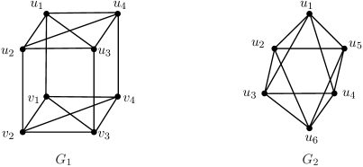
Figure 3.3: The underlying graphs containing triangles

Proof. Let $u_{1}u_{2}u_{3}u_{1}$ be a triangle in $G$. Since $u_{2}\in N(u_{1})\cap N(u_{3})$, there is another common neighbor between $u_{1}$ and $u_{3}$ from Proposition 2.2, denoted by $u_{4}$. Observe that $u_{3}\in N(u_{1})\cap N(u_{2})$. Then by Proposition 2.2 again, there is another vertex in $N(u_{1})\cap N(u_{2})$, which is either $u_{4}$ or a new vertex, say $u_{5}$.

Firstly, assume that $u_{4}\in N(u_{1})\cap N(u_{2})$, that is, $(u_{2},u_{4})\in G$. As $G$ is $4$-regular, $u_{1}$ has the fourth neighbor, denoted by $v_{1}$. We claim that $(v_{1},u_{2})\notin G$; otherwise $N(u_{1})\cap N(u_{2})=\{u_{3},u_{4},v_{1}\}$ which contradicts Proposition 2.2. Similarly, we have $(v_{1},u_{3})\notin G$ and $(v_{1},u_{4})\notin G$. We can further obtain that the new vertices $v_{2},v_{3}$ and $v_{4}$ are the forth neighbors of $u_{2},u_{3}$ and $u_{4}$, respectively, and $(v_{i},u_{j})\notin G$ for $1\leq i\neq j\leq 4$. Then we consider $N(v_{1})\cap N(u_{2})$. Note that $u_{1}\in N(u_{2})\cap N(v_{1})$, $(v_{1},u_{3})\notin G$ and $(v_{1},u_{4})\notin G$ by the discussion above, which forces that $v_{2}$ becomes another common neighbor between $v_{1}$ and $u_{2}$, i.e., $(v_{1},v_{2})\in G$. By similar discussions on $N(v_{1})\cap N(u_{4})$, $N(v_{3})\cap N(u_{2})$ and $N(v_{3})\cap N(u_{4})$, respectively, we can deduce that $(v_{1},v_{4})\in G$, $(v_{2},v_{3})\in G$ and $(v_{3},v_{4})\in G$. Noticing that $u_{1}\in N(v_{1})\cap N(u_{3})$, another common vertex must be $v_{3}$, since $d(u_{3})=4$ and the degrees of other neighbors of $u_{3}$ other than $v_{3}$ are equal to $4$. By considering $N(u_{2})\cap N(v_{4})$ similarly, we have $(v_{2},v_{4})\in G$. Up to now, the degrees of all vertices of $G$ attain $4$. Hence the underlying graph $G$ is the graph $G_{1}$ given in Figure 3.3.

Now we suppose that $N(u_{1})\cap N(u_{2})$ contains a new vertex $u_{5}$. We claim that $(u_{2},u_{4})\notin G$ and $(u_{3},u_{5})\notin G$; otherwise, $N(u_{1})\cap N(u_{2})=\{u_{3},u_{4},u_{5}\}$ or $N(u_{1})\cap N(u_{3})=\{u_{2},u_{4},u_{5}\}$, a contradiction to Proposition 2.2. Notice that $u_{3}\in N(u_{1})\cap N(u_{4})$, $d(u_{1})=4$ and $(u_{2},u_{4})\notin G$, which implies $(u_{4},u_{5})\in G$. Since $d(u_{5})=3$ and $(u_{3},u_{5})\notin G$, $u_{5}$ has the forth neighbor $u_{6}$. Now we consider $N(u_{2})\cap N(u_{5})$. Combining the observation that $u_{1}\in N(u_{2})\cap N(u_{5})$ with the fact $(u_{2},u_{4})\notin G$, we deduce that $u_{6}\in N(u_{2})\cap N(u_{5})$. Then by a similar way, we successively discuss $N(u_{2})\cap N(u_{3})$ and $N(u_{3})\cap N(u_{4})$ and obtain $(u_{3},u_{6})\in G$ and $(u_{4},u_{6})\in G$. It is easy to check that the graph has already been $4$-regular and is just the graph $G_{2}$ depicted in Figure 3.3.  

Theorem 3.2

Let $G^{\sigma}$ be a $4$-regular oriented graph with optimum skew energy. If the underlying graph $G$ is triangle-free, then $G$ is one of the following graphs: the hypercube $Q_{4}$ of dimension $4$, the graph $G_{3}$, a graph in $\mathcal{G}_{i}$, or a graph in $\mathcal{H}_{j}$; see Figures 2.1, 2.2 and 3.4.

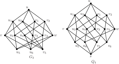
Figure 3.4: The underlying graphs containing no triangles

Proof. Let $u_{1},u_{2},v_{1}$ and $v_{2}$ be all neighbors of a vertex $u$ in $G$. Then the induced subgraph $G[\{u_{1},u_{2},v_{1},v_{2}\}]$ contains no edge, since the graph $G$ is triangle-free. Denote by $v,u_{3},u_{4}$ be another three neighbors of $u_{1}$ other than $u$. Note that $u_{1}\in N(u)\cap N(v)$. By Proposition 2.2, there is another one or three common neighbors in $\{u_{2},v_{1},v_{2}\}$ between $u$ and $v$. We can obtain the same results by considering $N(u)\cap N(u_{3})$ and $N(u)\cap N(u_{4})$. Assume that $a_{1},a_{2}$ and $a_{3}$ are the numbers of the common neighbors in $\{u_{2},v_{1},v_{2}\}$ between $u$ and $v$, $u$ and $u_{3}$, $u$ and $u_{4}$, respectively. Obviously, $a_{1},a_{2},a_{3}\in\{1,3\}$. Without loss of generality, suppose $a_{1}\geq a_{2}\geq a_{3}$. We discuss the following four cases according to the values of $a_{1},a_{2}$ and $a_{3}$.

Case 1. $(a_{1},a_{2},a_{3})=(1,1,1)$.

Without loss of generality, let $(u_{2},v)\in G$. Then $(v_{1},v)\notin G$ and $(v_{2},v)\notin G$ as $a_{1}=1$. Observe that $u\in N(u_{1})\cap N(v_{1})$, which implies that there is another common neighbor in $\{u_{3},u_{4}\}$ between $u_{1}$ and $v_{1}$. Let $u_{3}\in N(u_{1})\cap N(v_{1})$. Then $(u_{2},u_{3})\notin G$ and $(v_{2},u_{3})\notin G$ as $a_{2}=1$. By considering $N(u_{1})\cap N(v_{2})$, we deduce that $(v_{2},u_{4})\in G$, since $(v_{2},v)\notin G$ and $(v_{2},u_{3})\notin G$ by the discussion above. Obviously, $(u_{2},u_{4})\notin G$ and $(v_{2},u_{4})\notin G$ as $a_{3}=1$. Then it is known that $u_{2}$ contains another two neighbors, say $v_{3}$ and $v_{4}$. Since $u\in N(u_{2})\cap N(v_{1})$ and $(v_{1},v)\notin G$, it follows that there is another common neighbor in $\{v_{3},v_{4}\}$ between $u_{2}$ and $v_{1}$. Without loss of generality, $v_{3}\in N(u_{2})\cap N(v_{1})$. Then $(v_{1},v_{4})\notin G$; otherwise, $|N(u_{2})\cap N(v_{1})|=3$ and no other vertex can be chosen as the forth common neighbor, which is a contradiction. In view of the observation that $u\in N(u_{2})\cap N(v_{2})$ and $(v_{2},v)\notin G$, we have that another common neighbor between $u_{2}$ and $v_{2}$ belongs to $\{v_{3},v_{4}\}$. We claim that $v_{3}\notin N(u_{2})\cap N(v_{2})$; otherwise, $N(u)\cap N(v_{3})=\{u_{2},v_{1},v_{2}\}$ and there is no other vertex in $N(u)\cap N(v_{3})$, which contradicts Proposition 2.2. Therefore, $v_{4}\in N(u_{2})\cap N(v_{2})$. We proceed to have $w$ as the forth neighbor of $v_{1}$. By considering $N(v_{1})\cap N(v_{2})$, we obtain $(v_{2},w)\in G$.

Up to now, we have $d(u)=d(u_{1})=d(u_{2})=d(v_{1})=d(v_{2})=4$ and $d(v)=d(u_{3})=d(u_{4})=d(v_{3})=d(v_{4})=d(w)=3$. We claim that the deduced subgraph $G[\{v,u_{3},u_{4},v_{3},v_{4},w\}]$ is empty. Otherwise, the possible edges are $(v,w),(u_{3},v_{4})$ and $(u_{4},v_{3})$ since $G$ is triangle-free. If $(v,w)\in G$, then $|N(u_{1})\cap N(w)|=1$, which is a contradiction. We thus have $(v,w)\notin G$. Similarly, $(u_{3},v_{4})\notin G$ and $(u_{4},v_{3})\notin G$.

Suppose now that $u_{5}$ and $u_{6}$ are the other two neighbors of $v$. Note that $u_{1}\in N(v)\cap N(u_{3})$. Then we have either $(u_{3},u_{5})\in G$ or $(u_{3},u_{6})\in G$. Without loss of generality, $(u_{3},u_{5})\in G$, and hence $(u_{3},u_{6})\notin G$. Moreover, $(u_{4},u_{5})\notin G$, otherwise, $N(u_{1})\cap N(u_{5})=\{v,u_{3},u_{4}\}$, a contradiction. By considering $N(u_{1})\cap N(u_{6})$, we get $(u_{4},u_{6})\in G$. Assume that $v_{5}$ is the forth neighbor of $u_{3}$. It is obvious that $u_{3}\in N(u_{1})\cap N(v_{5})$, which forces that $u_{4}$ becomes another common vertex between $u_{1}$ and $v_{5}$. We see that $v\in N(u_{2})\cap N(u_{5})$, which indicates that there is another common neighbor between $u_{2}$ and $u_{5}$. It means either $(v_{3},u_{5})\in G$ or $(v_{4},u_{5})\in G$. We discuss the two cases separately.

On the one hand, if $(v_{3},u_{5})\in G$, then $(v_{4},u_{5})\notin G$. It follows that $(v_{4},u_{6})\in G$ by considering $N(v)\cap N(v_{4})$. We claim that $(v_{3},u_{6})\notin G$ and $(v_{3},v_{5})\notin G$; otherwise, $N(v)\cap N(v_{3})=\{u_{2},u_{5},u_{6}\}$ or $N(u_{3})\cap N(v_{3})=\{v_{1},u_{5},v_{5}\}$, which is a contradiction. Therefore, $v_{3}$ contains a new neighbor, denoted by $v_{6}$. Since $v_{3}\in N(v_{1})\cap N(v_{6})$, we have $(w,v_{6})\in G$, since $w$ is the unique neighbor of $v_{1}$ with degree less than $4$. Similarly, we get $(v_{4},v_{6})\in G$ by considering $N(v_{2})\cap N(v_{6})$. We further obtain that $(w,v_{5})\in G$ by considering $N(v_{2})\cap N(v_{5})$.

Up to now, $d(u_{5})=d(u_{6})=d(v_{5})=d(v_{6})=3$ and other vertices above have degree $4$. It is known that $G[\{u_{5},u_{6},v_{5},v_{6}\}]$ contains no edges because of the triangle-free property of $G$. Suppose now that $s$ is the forth neighbor of $u_{5}$. Considering $N(v)\cap N(s)$, $N(u_{3})\cap N(s)$ and $N(v_{3})\cap N(s)$, respectively, we derive that $(u_{5},s)\in G,(u_{6},s)\in G,(v_{5},s)\in G$ and $(v_{6},s)\in G$. Now all vertices have degree $4$. It can be verified that $G$ is the hypercube $Q_{4}$.

On the other hand, $(v_{4},u_{5})\in G$. It follows that $v_{4}\in N(v_{2})\cap N(u_{5})$. Then we have $(w,u_{5})\in G$, since $w$ is the unique neighbor of $v_{2}$ with degree less than $4$ other than $v_{4}$. Note that $u_{2}\in N(v)\cap N(v_{3})$, which forces that $u_{6}$ becomes another common neighbor between $v$ and $v_{3}$, since $u_{6}$ is the unique neighbor of $v$, whose degree is less than $4$. By a similar discussion on $N(u_{3})\cap N(v_{3})$, we can deduce that $(v_{3},v_{5})\in G$. Since $u_{5}\in N(u_{3})\cap N(v_{4})$, we get $(v_{4},v_{5})\in G$. We further consider $N(u_{4})\cap N(w)$ and obtain $(w,u_{6})\in G$. Now all vertices have degree $4$. It can be easily verified that $G$ is the graph $G_{3}$ depicted in Figure 3.4.

Case 2. $(a_{1},a_{2},a_{3})=(3,1,1)$.

In this case, $v$ is adjacent to all vertices of $\{u_{2},v_{1},v_{2}\}$, while $u_{3}$ and $u_{4}$ are adjacent to one of them, respectively. Without loss of generality, $(u_{2},u_{3})\in G$. Then $(v_{1},u_{3})\notin G$ and $(v_{2},u_{3})\notin G$ since $a_{2}=1$. It follows that $(u_{2},u_{4})\in G$. If not, then either $(v_{1},u_{4})\in G$ or $(v_{2},u_{4})\in G$, where the former possibility implies that $N((u_{1})\cap N(v_{1})=\{u,v,u_{4}\})$ and the latter implies that $N(u_{1})\cap N(v_{2})=\{u,v,u_{4}\}$, both of which contradict Proposition 2.2. Hence $(u_{2},u_{4})\in G$, $(v_{1},u_{4})\notin G$ and $(v_{2},u_{4})\notin G$. Now let $v_{3}$ and $v_{4}$ be another two neighbors of $v_{1}$. Observe that $v_{1}\in N(v)\cap N(v_{3})$, which forces $v_{2}$ to be another common vertex between $v$ and $v_{3}$. By a similar discussion on $N(v)\cap N(v_{4})$, we can derive $(v_{2},v_{4})\in G$.

Now, $d(u)=d(v)=d(u_{1})=d(u_{2})=d(v_{1})=d(v_{2})=4$ and $d(u_{3})=d(u_{4})=d(v_{3})=d(v_{4})=2$. We can divide our subsequent discussion into the following steps.

1. If the induced subgraph $G[\{u_{3},u_{4},v_{3},v_{4}\}]$ contains edges, then the edges can only be some of $(u_{3},v_{3})$, $(u_{4},v_{4})$, $(u_{3},v_{4})$ and $(u_{4},v_{3})$, since $G$ is triangle-free. Without loss generality, assume $(u_{3},v_{4})\in G$. Then $u_{3}\in N(u_{1})\cap N(v_{4})$ and $v_{4}\in N(v_{2})\cap N(u_{3})$, which forces $(u_{4},v_{4})\in G$ and $(u_{3},v_{3})\in G$. We further consider $N(u_{2})\cap N(v_{3})$, and obtain $(u_{4},v_{3})\in G$. Consequently, each vertex above has degree $4$. It is easy to verify that $G$ is the graph $\mathcal{G}_{1}$ depicted in Figure 2.1. Now the discussion stop;

2. If the induced subgraph $G[\{u_{3},u_{4},v_{3},v_{4}\}]$ contains no edges, then there are another two neighbors of $u_{3}$, say $u_{5}$ and $u_{6}$. Considering $N(u_{1})\cap N(u_{5})$ and $N(u_{1})\cap N(u_{6})$, respectively, we have $(u_{4},u_{5})\in G$ and $(u_{4},u_{6})\in G$, since $u_{4}$ is the unique neighbor of $u_{1}$ whose degree is less than $4$.
   On the one hand, if $u_{5}$ or $u_{6}$ is adjacent to $v_{3}$ or $v_{4}$, then without loss generality we can suppose $(u_{5},v_{3})\in G$. Then $v_{3}\in N(v_{1})\cap N(u_{5})$, which implies $(u_{5},v_{4})\in G$. Notice that $u_{5}\in N(u_{3})\cap N(v_{3})$ and $u_{5}\in N(u_{3})\cap N(v_{4})$. Then we deduce that $(v_{3},u_{6})\in G$ and $(v_{4},u_{6})\in G$, since $u_{6}$ is the unique neighbor of $u_{3}$ whose degree is less than $4$. It can be verified that $G$ is the graph $\mathcal{H}_{2}$ depicted in Figure 2.2.
   On the other hand, both $u_{5}$ and $u_{6}$ are not adjacent to $v_{3}$ or $v_{4}$. Then $v_{3}$ has another two neighbors, denoted by $v_{5}$ and $v_{6}$. By a similar discussion on $N(v_{2})\cap N(v_{5})$ and $N(v_{2})\cap N(v_{6})$, respectively, we can obtain $(v_{4},v_{5})\in G$ and $(v_{4},v_{6})\in G$. Then continue the following step;

3. If the induced subgraph $G[\{u_{5},u_{6},v_{5},v_{6}\}]$ contains edges, we can discuss this case similar to Step $1$. Consequently, we can obtain that $G$ is the graph $\mathcal{G}_{2}$ depicted in Figure 2.1. The discussion stops; If the induced subgraph $G[\{u_{5},u_{6},v_{5},v_{6}\}]$ contains no edges, we can also continue the discussion according to Step $2$, until we get that $G$ is the graph $\mathcal{H}_{3}$ depicted in Figure 2.2, or executing Step $3$ again. The discussion continues.

It should be pointed out that the discussion will terminate by illustrating that $G$ is either a graph in $\mathcal{G}_{i}$ or a graph in $\mathcal{H}_{j}$, which are shown in Figure 2.1 and Figure 2.2, respectively.

Case 3. $(a_{1},a_{2},a_{3})=(3,3,1)$.

This case means that $v$ and $u_{3}$ are adjacent to all vertices of $\{u_{2},v_{1},v_{2}\}$, while $u_{4}$ is precisely adjacent to one of them. Without loss generality, suppose $(u_{2},u_{4})\in G$. Then $(v_{1},u_{4})\notin G$ and $(v_{2},u_{4})\notin G$. Consequently, $|N(u_{1})\cap N(v_{1})|=|\{u,v,u_{3}\}|=3$, which contradicts Proposition 2.2. Therefore, this case could not happen.

Case 4. $(a_{1},a_{2},a_{3})=(3,3,3)$.

Obviously, $v$, $u_{3}$ and $u_{4}$ are adjacent to all vertices of $\{u_{2},v_{1},v_{2}\}$. It can be checked that all vertices have degree $4$, and hence $G$ is the complete bipartite graph $K_{4,4}$, which is also the graph $\mathcal{H}_{1}$ depicted in Figure 2.2.

To sum up the discussion above, $G$ is the hypercube $Q_{4}$ or the graph $G_{3}$ or a graph in $\mathcal{G}_{i}$ or a graph in $\mathcal{H}_{j}$. The proof is now complete.  

For convenience, we denote the set of all graphs presented above by $\mathcal{F}$, which consists of $G_{1}$, $G_{2}$, $G_{3}$, $Q_{4}$, all graphs in $\mathcal{G}_{i}$ and all graphs in $\mathcal{H}_{j}$. Combining Theorem 3.1 with Theorem 3.2, we conclude one of our main results as follows.

Theorem 3.3

Let $G^{\sigma}$ be a $4$-regular oriented graph with optimum skew energy. Then the underlying graph $G$ is a graph in $\mathcal{F}$.

Now the question naturally arises: whether there exists an orientation for each graph of $\mathcal{F}$ such that the resultant oriented graph attains optimum skew energy. The following results tell us that for each graph of $\mathcal{F}$ such orientation indeed exists.

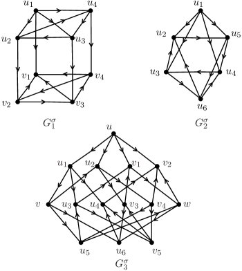
Figure 3.5: The optimum orientations for $G_{1}$, $G_{2}$ and $G_{3}$

Theorem 3.4

Let $G_{1}^{\sigma}$, $G_{2}^{\sigma}$ and $G_{3}^{\sigma}$ be the oriented graphs of $G_{1}$, $G_{2}$ and $G_{3}$, respectively, given in Figure 3.5. Then each of them has the optimum shew energy.

Proof. Let the rows of the skew-adjacency matrix $S(G_{1}^{\sigma})$ correspond successively the vertices $u_{1}$, $u_{2}$, $u_{3}$, $u_{4}$, $v_{1}$, $v_{2}$, $v_{3}$ and $v_{4}$. It follows that

$$S(G_{1}^{\sigma})=\begin{bmatrix}0&1&1&1&1&0&0&0\\ -1&0&-1&1&0&1&0&0\\ -1&1&0&-1&0&0&1&0\\ -1&-1&1&0&0&0&0&1\\ -1&0&0&0&0&-1&-1&-1\\ 0&-1&0&0&1&0&1&-1\\ 0&0&-1&0&1&-1&0&1\\ 0&0&0&-1&1&1&-1&0\\ \end{bmatrix}$$

Let the rows of the skew-adjacency matrix $S(G_{2}^{\sigma})$ correspond successively the vertices $u_{1}$, $u_{2}$, $u_{3}$, $u_{4}$, $u_{5}$ and $u_{6}$. Then

$$S(G_{2}^{\sigma})=\begin{bmatrix}0&1&1&1&1&0\\ -1&0&-1&0&1&-1\\ -1&1&0&-1&0&1\\ -1&0&1&0&-1&-1\\ -1&-1&0&1&0&1\\ 0&1&-1&1&-1&0\\ \end{bmatrix}$$

Similarly, let the rows of the skew-adjacency matrix $S(G_{3}^{\sigma})$ correspond successively the vertices $u$, $u_{1}$, $u_{2}$, $v_{1}$, $v_{2}$, $v$, $u_{3}$, $u_{4}$, $v_{3}$, $v_{4}$, $w$, $u_{5}$, $u_{6}$ and $v_{5}$. Then

$$S(G_{3}^{\sigma})=\setcounter{MaxMatrixCols}{14}\begin{bmatrix}0&1&1&1&1&0&0&0&0&0&0&0&0&0\\ -1&0&0&0&0&1&1&1&0&0&0&0&0&0\\ -1&0&0&0&0&-1&0&0&1&1&0&0&0&0\\ -1&0&0&0&0&0&-1&0&-1&0&1&0&0&0\\ -1&0&0&0&0&0&0&-1&0&-1&-1&0&0&0\\ 0&-1&1&0&0&0&0&0&0&0&0&1&1&0\\ 0&-1&0&1&0&0&0&0&0&0&0&-1&0&1\\ 0&-1&0&0&1&0&0&0&0&0&0&0&-1&-1\\ 0&0&-1&1&0&0&0&0&0&0&0&0&1&-1\\ 0&0&-1&0&1&0&0&0&0&0&0&1&0&1\\ 0&0&0&-1&1&0&0&0&0&0&0&-1&1&0\\ 0&0&0&0&0&-1&1&0&0&-1&1&0&0&0\\ 0&0&0&0&0&-1&0&1&-1&0&-1&0&0&0\\ 0&0&0&0&0&0&-1&1&1&-1&0&0&0&0\\ \end{bmatrix}$$

It is not difficult to check that $S(G_{1}^{\sigma})^{T}S(G_{1}^{\sigma})=4I_{8}$, $S(G_{2}^{\sigma})^{T}S(G_{2}^{\sigma})=4I_{6}$ and $S(G_{3}^{\sigma})^{T}S(G_{3}^{\sigma})=4I_{14}$. We can also verify these equalities by proving that different row vectors of each of $S(G_{1}^{\sigma})$, $S(G_{2}^{\sigma})$ and $S(G_{3}^{\sigma})$ are pairwise orthogonal. The theorem is thus proved.  

We have known from [11] that there exists an orientation $\sigma$ of $Q_{4}$ such that the resultant oriented graph $Q_{4}^{\sigma}$ has optimum skew energy. The following two algorithms recursively describe optimum orientations of $\mathcal{G}_{i}$ and $\mathcal{H}_{j}$, respectively.

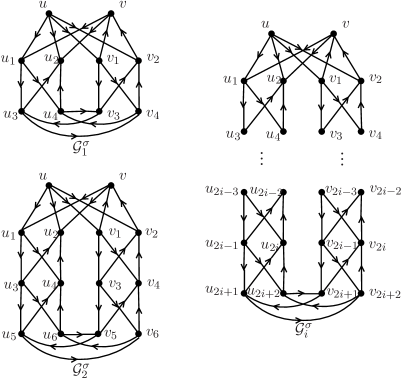
Figure 3.6: The optimum orientation for $\mathcal{G}_{i}$

Algorithm 1.

1. Give $\mathcal{G}_{1}$ an orientation as shown in Figure 3.6.

2. Assume that $\mathcal{G}_{1},\mathcal{G}_{2},\dots,\mathcal{G}_{t-1}$ have been oriented into $\mathcal{G}_{1}^{\sigma},\mathcal{G}_{2}^{\sigma},\dots,\mathcal{G}_{t-1}^{\sigma}$. Then we orient $\mathcal{G}_{t}$ with the following method:

   1. Keep the orientations of all edges in $E(\mathcal{G}_{t-1})\cap E(\mathcal{G}_{t})$.

   2. Give the remaining edges orientations such that $\langle u_{2t-1},u_{2t+1}\rangle$, $\langle u_{2t-1},u_{2t+2}\rangle$, $\langle u_{2t+1},u_{2t}\rangle$, $\langle u_{2t+2},u_{2t}\rangle$, $\langle v_{2t-1},v_{2t+1}\rangle$, $\langle v_{2t-1},v_{2t+2}\rangle$, $\langle v_{2t+1},v_{2t}\rangle$, $\langle v_{2t+2},v_{2t}\rangle$, $\langle u_{2t+1},v_{2t+2}\rangle$, $\langle v_{2t+2},u_{2t+2}\rangle$, $\langle u_{2t+2},v_{2t+1}\rangle$ and $\langle v_{2t+1},u_{2t+1}\rangle$ belong to $\Gamma(\mathcal{G}_{t}^{\sigma})$.

3. If $t=i$, stop; else take $t-1:=t$, return to Step 2.

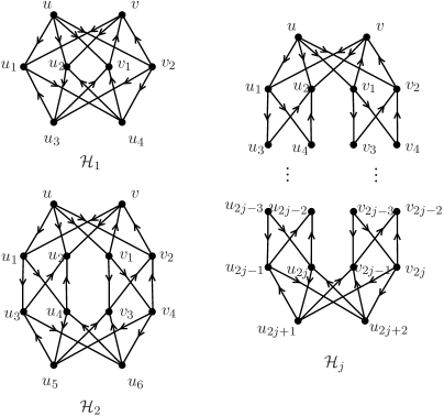
Figure 3.7: The optimum orientation for $\mathcal{H}_{j}$

Algorithm 2.

1. Give $\mathcal{H}_{1}$ an orientation as shown in Figure 3.7.

2. Assume that $\mathcal{H}_{1},\mathcal{H}_{2},\dots,\mathcal{H}_{t-1}$ have been oriented into $\mathcal{H}_{1}^{\sigma},\mathcal{H}_{2}^{\sigma},\dots,\mathcal{H}_{t-1}^{\sigma}$. Then we orient $\mathcal{H}_{t}$ with the following method:

   1. Keep the orientations of all edges in $E(\mathcal{H}_{t-1})$$\cap E(\mathcal{H}_{t})$$\backslash$$\{(u_{2t-3},u_{2t-1}),(u_{2t-3},u_{2t}),$
      $(u_{2t-2},u_{2t-1}),(u_{2t-2},u_{2t})\}$.

   2. Give the remaining edges orientations such that $\langle u_{2t-3},u_{2t-1}\rangle$, $\langle u_{2t-3},u_{2t}\rangle$, $\langle u_{2t-1},u_{2t-2}\rangle$, $\langle u_{2t},u_{2t-2}\rangle$, $\langle v_{2t-3},v_{2t-1}\rangle$, $\langle v_{2t-3},v_{2t}\rangle$, $\langle v_{2t-1},v_{2t-2}\rangle$, $\langle v_{2t},v_{2t-2}\rangle$, $\langle u_{2t+1},u_{2t-1}\rangle$, $\langle u_{2t-1},u_{2t+2}\rangle$, $\langle u_{2t},u_{2t+1}\rangle$, $\langle u_{2t+2},u_{2t}\rangle$, $\langle u_{2t+1},v_{2t-1}\rangle$, $\langle u_{2t+2},v_{2t-1}\rangle$ $\langle v_{2t},u_{2t+1}\rangle$ and $\langle v_{2t},u_{2t+2}\rangle$ belong to $\Gamma(\mathcal{H}_{t}^{\sigma})$.

3. If $t=i$, stop; else take $t-1:=t$, return to Step 2.

Next, we shall prove that $\mathcal{G}_{i}^{\sigma}$ and $\mathcal{H}_{j}^{\sigma}$ derived from Algorithm 1 and Algorithm 2, respectively, have optimum skew energy, that is, their skew-adjacency matrices satisfy $S(\mathcal{G}_{i}^{\sigma})^{T}S(\mathcal{G}_{i}^{\sigma})=4I$ and $S(\mathcal{H}_{j}^{\sigma})^{T}S(\mathcal{H}_{j}^{\sigma})=4I$. In order to illustrate clearly the skew-adjacency matrices $S(\mathcal{G}_{i}^{\sigma})$ and $S(\mathcal{H}_{j}^{\sigma})$, we here define some small matrix blocks.

$$A =\begin{bmatrix}1&1&1&1\\ 1&1&-1&-1\\ \end{bmatrix} \hskip 25.0ptB =\begin{bmatrix}1&1&0&0\\ -1&-1&0&0\\ 0&0&1&1\\ 0&0&-1&-1\\ \end{bmatrix}$$

$$C =\begin{bmatrix}0&0&-1&1\\ 0&0&1&-1\\ 1&-1&0&0\\ -1&1&0&0\\ \end{bmatrix} \hskip 25.0ptD =\begin{bmatrix}-1&1\\ 1&-1\\ -1&-1\\ 1&1\\ \end{bmatrix}$$

Theorem 3.5

Let $S(\mathcal{G}_{i}^{\sigma})$ be the skew-adjacency matrix of $\mathcal{G}_{i}^{\sigma}$ obtained from Algorithm 1. Then $S(\mathcal{G}_{i}^{\sigma})^{T}S(\mathcal{G}_{i}^{\sigma})=4I$.

Proof. Let the rows of the skew-adjacency matrix $S(\mathcal{G}_{i})$ correspond successively the vertices $u$, $v$, $u_{1}$, $u_{2}$, $v_{1}$, $v_{2}$, $\dots$, $u_{2i+1}$, $u_{2i+2}$, $v_{2i+1}$, $v_{2i+2}$. Then from Algorithm 1, $S(\mathcal{G}_{i})$ can be written as the block matrix for each positive integer $i$.

For $i=1$ and $i=2$,

$$S(\mathcal{G}_{1}^{\sigma})=\begin{bmatrix}0&A&0\\ -A^{T}&0&B\\ 0&-B^{T}&C\end{bmatrix} \hskip 25.0ptS(\mathcal{G}_{2}^{\sigma})=\begin{bmatrix}0&A&0&0\\ -A^{T}&0&B&0\\ 0&-B^{T}&0&B\\ 0&0&-B^{T}&C\end{bmatrix}$$

By applying multiplication of block matrix, it is easy to compute that

$$S(\mathcal{G}_{1}^{\sigma})^{T}S(\mathcal{G}_{1}^{\sigma}) =\begin{bmatrix}AA^{T}&0&-AB\\ 0&A^{T}A+BB^{T}&-BC\\ -B^{T}A^{T}&-C^{T}B^{T}&B^{T}B+C^{T}C\end{bmatrix}$$

$$S(\mathcal{G}_{2}^{\sigma})^{T}S(\mathcal{G}_{2}^{\sigma}) =\begin{bmatrix}AA^{T}&0&-AB&0\\ 0&A^{T}A+BB^{T}&0&-B^{2}\\ -B^{T}A^{T}&0&B^{T}B+BB^{T}&-BC\\ 0&-(B^{T})^{2}&-C^{T}B^{T}&B^{T}B+C^{T}C\end{bmatrix}$$

In order to prove $S(\mathcal{G}_{1}^{\sigma})^{T}S(\mathcal{G}_{1}^{\sigma})=4I$ and $S(\mathcal{G}_{2}^{\sigma})^{T}S(\mathcal{G}_{2}^{\sigma})=4I$, it suffices to prove that the following equalities meanwhile hold.

$$\begin{split}&AA^{T}=4I_{2},\,\,A^{T}A+BB^{T}=4I_{4},\,\,B^{T}B+BB^{T}=4I_{4},\\ &B^{T}B+C^{T}C=4I_{4},\,\,AB=0,\,\,B^{2}=0,\,\,BC=0.\end{split}$$ (3.1)

By the definitions of $A$, $B$ and $C$, it is easy to verify that all equalities 3.1 indeed hold. In fact, these equalities can further guarantee $S(\mathcal{G}_{i}^{\sigma})^{T}S(\mathcal{G}_{i}^{\sigma})=4I$, because $S(\mathcal{G}_{i})$ can be formulated as

$$S(\mathcal{G}_{i}^{\sigma})=\left[\begin{array}[]{ccccccc}0&A&0&0&\cdots&0&0\\ -A^{T}&0&B&0&\cdots&0&0\\ 0&-B^{T}&0&B&\cdots&0&0\\ 0&0&-B^{T}&0&\cdots&0&0\\ \vdots&\vdots&\vdots&\vdots&\vdots&\vdots&\vdots\\ 0&0&0&0&\cdots&0&B\\ 0&0&0&0&\cdots&-B^{T}&C\\ \end{array}\right].$$

It should be pointed out that if one only considers $\mathcal{G}_{1}$, then it is enough to check that parts of the equalities hold. The proof is now complete.  

Theorem 3.6

Let $S(\mathcal{H}_{j}^{\sigma})$ be the skew-adjacency matrix of $\mathcal{H}_{j}^{\sigma}$ obtained from Algorithm 2. Then $S(\mathcal{H}_{j}^{\sigma})^{T}S(\mathcal{H}_{j}^{\sigma})=4I$.

Proof. Similar to the proof of Theorem 3.5, let the rows of the skew-adjacency matrix $S(\mathcal{H}_{j})$ correspond successively the vertices $u$, $v$, $u_{1}$, $u_{2}$, $v_{1}$, $v_{2}$, $\dots$, $u_{2i-1}$, $u_{2i}$, $v_{2i-1}$, $v_{2i}$, $u_{2i+1}$ and $u_{2i+2}$.

$$S(\mathcal{H}_{1}^{\sigma})=\begin{bmatrix}0&A&0\\ -A^{T}&0&D\\ 0&-D^{T}&0\end{bmatrix} \hskip 25.0ptS(\mathcal{H}_{2}^{\sigma})=\begin{bmatrix}0&A&0&0\\ -A^{T}&0&B&0\\ 0&-B^{T}&0&D\\ 0&0&-D^{T}&0\end{bmatrix}$$

$$S(\mathcal{H}_{j}^{\sigma})=\left[\begin{array}[]{cccccccc}0&A&0&0&\cdots&0&0&0\\ -A^{T}&0&B&0&\cdots&0&0&0\\ 0&-B^{T}&0&B&\cdots&0&0&0\\ 0&0&-B^{T}&0&\cdots&0&0&0\\ \vdots&\vdots&\vdots&\vdots&\vdots&\vdots&\vdots&\vdots\\ 0&0&0&0&\cdots&0&B&0\\ 0&0&0&0&\cdots&-B^{T}&0&D\\ 0&0&0&0&\cdots&0&-D^{T}&0\\ \end{array}\right]$$

We can verify that $S(\mathcal{H}_{1})^{T}S(\mathcal{H}_{1})=4I$ if and only if the equalities below hold,

$$AA^{T}=4I_{2},\,\,A^{T}A+DD^{T}=4I_{4},\,\,D^{T}D=4I_{2},\,\,AD=0.$$ (3.2)

while $S(\mathcal{H}_{2})^{T}S(\mathcal{H}_{2})=4I$ if and only if the following equalities hold,

$$\begin{split}&AA^{T}=4I_{2},\,\,A^{T}A+BB^{T}=4I_{4},\,\,B^{T}B+D^{T}D=4I_{4},\\ &D^{T}D=4I_{2},\,\,AB=0,\,\,BD=0.\end{split}$$ (3.3)

For $j\geq 3$, combining equalities in (3.3) with equalities $B^{T}B+BB^{T}=4I_{4}$ and $B^{2}=0$, it is enough to ensure that the equality $S(\mathcal{H}_{j}^{\sigma})^{T}S(\mathcal{H}_{j}^{\sigma})=4I$ holds.

By the definitions of $A,B$ and $D$, it can be directly checked that the all equalities above indeed hold. This completes the proof.  

We can summarize all results above as the following theorem.

Theorem 3.7

Let $G$ be a $4$-regular graph. Then $G$ has an optimum orientation if and only if $G$ is a graph of $\mathcal{F}$.

Remark 1. For arbitrary matrices $A^{\prime}$, $B^{\prime}$, $C^{\prime}$ and $D^{\prime}$ with entries $0$, $1$ and $-1$, if they have the same orders and the same number of $0^{\prime}$s with $A$, $B$, $C$ and $D$, respectively, and meanwhile they satisfy all the equalities of Theorem 3.5 and Theorem 3.6, then we can substitute $A$, $B$, $C$ and $D$, respectively by $A^{\prime}$, $B^{\prime}$, $C^{\prime}$ and $D^{\prime}$ in the skew-adjacency matrices $S(\mathcal{G}_{i})$ and $S(\mathcal{H}_{j})$, and the corresponding oriented graphs still have optimum skew energy.

Remark 2. The proofs of Theorem 3.5 and Theorem 3.6 are based on matrix computations by proving that the skew-adjacency matrix $S$ satisfies $S^{T}S=nI$. Besides, we can apply Proposition 2.4 to prove that for any two distinct vertices $u$ and $v$, the number of all positive walks equals that of all negative walks from $u$ to $v$ with length $2$.

References

- [1] C. Adiga, R. Balakrishnan, W. So, The shew energy of a digraph, Linear Algebra Appl. 432(2010), 1825–1835.
- [2] X. Chen, X. Li, H. Lian, The skew energy of random oriented graphs, Linear Algebra Appl. 438(2013), 4547–4556.
- [3] S. Gong, G. Xu, -Regular digraphs with optimum skew energy, Linear Algebra Appl. 436(2012), 465–471.
- [4] I. Gutman, The energy of a graph, Ber. Math. Statist. Sekt. Forschungsz. Graz, 103(1978), 1–22.
- [5] I. Gutman, X. Li, J. Zhang, Graph Energy, in: M. Dehmer, F. Emmert-Streib (Eds.), Analysis of Complex Network: From Biology to Linguistics, Wiley-VCH Verlag, Weinheim, 2009, 145–174.
- [6] Y. Hou, T. Lei, Characteristic polynomials of skew-adjacency matrices of oriented graphs, Electron. J. Combin. 18(2011), 156–167.
- [7] Y. Hou, X. Shen, C. Zhang, Oriented unicyclic graphs with extremal skew energy, Available at http://arxiv.org/abs/1108.6229.
- [8] X. Li, Y. Shi, I. Gutman, Graph Energy, Springer, New York, 2012.
- [9] B. Shader, W. So, Skew spectra of oriented graphs, Electron. J. Combin. 16(2009), #N32.
- [10] X. Shen, Y. Hou, C. Zhang, Bicyclic digraphs with extremal skew energy, Electron. J. Linear Algebra 23(2012), 340–355.
- [11] G. Tian, On the skew energy of orientations of hypercubes, Linear Algebra Appl. 435(2011), 2140–2149.