Continuous- and discrete-time Glauber dynamics. First- and second-order phase transitions in mean-field Potts models

Abstract

As is known, at the Gibbs-Boltzmann equilibrium, the mean-field $q$-state Potts model with a ferromagnetic coupling has only a first order phase transition when $q\geq 3$, while there is no phase transition for an antiferromagnetic coupling. The same equilibrium is asymptotically reached when one considers the continuous time evolution according to a Glauber dynamics. In this paper we show that, when we consider instead the Potts model evolving according to a discrete-time dynamics, the Gibbs-Boltzmann equilibrium is reached only when the coupling is ferromagnetic while, when the coupling is anti-ferromagnetic, a period-2 orbit equilibrium is reached and a stable second-order phase transition in the Ising mean-field universality class sets in for each component of the orbit. We discuss the implications of this scenario in real-world problems.

1 Introduction

The $q$-state Potts model is one of the most important models in statistical physics [1]. For example, in the limit $q\to 1$, the model is equivalent to bond-percolation phenomena [2]. More in general, the model finds countless applications in computer science, like coloring a random graph [3, 4], and extracting communities from real-world networks [5] (for a review see also [6]). It is perhaps the first candidate model when one wants to consider first-order phase transition phenomena which, as opposed to second-order transitions, are characterized by a finite jump of the order parameter. In the mean-field version of the model, for example, where any spin interact with any other spin, it is easy to show that, at the Gibbs-Boltzmann equilibrium, when the number of states $q>2$, and the coupling is ferromagnetic, a first-order transition takes place while, for $q=2$, the model is equivalent to the Ising model and only a second-order phase transition takes place. When the coupling is instead anti-ferromagnetic, no phase transition sets in, for any $q$, and the system remains in its trivial symmetric solution. The same scenario is found when one uses a dynamical approach like the continuous-time Glauber dynamics [8]: after an initial transient time the systems reaches the Gibbs-Boltzmann equilibrium, in both the ferromagnetic and anti-ferromagnetic case.

In this paper, after reviewing the mean-field Potts model at equilibrium, and along the continuous-time Glauber dynamics, we introduce a discrete-time “Glauber” dynamics. We then show that, when the coupling is ferromagnetic, the differences between the continuous- and the discrete-time dynamics are irrelevant. However, when the coupling is anti-ferromagnetic, along the discrete-time dynamics the system reaches a dynamical stability by oscillating regularly between two values. In other words, when the dynamics is discrete and the coupling anti-ferromagnetic, the system never reaches a point-like equilibrium, but rather a period-2 stable trajectory. Moreover, there exists a critical temperature where the system undergoes a second-order phase transition in the mean-field Ising universality class, for any $q\geq 2$.

Perhaps, the reader familiar with the Ising model ($q=2$) will not find surprising that in the anti-ferromagnetic case a discrete-time dynamics can produce stable finite oscillations because, at any two dynamic iterations, the effective coupling becomes ferromagnetic. Ising models with a discrete-time dynamics were studied long ago in the context of 2-state neural networks and cellular automata and, later, also in the random field Ising model [13]. However, in the Potts case ($q>2$), we find out also the non intuitive feature that the nature of the phase transition changes dramatically: the fact that the effective coupling is ferromagnetic does not return a first-order phase transition, but a second-order phase transition.

Continuous phase transitions in the Potts model with $q\geq 3$ were observed in complex networks with power law exponent $\gamma\leq 3$ [6], and also on the complete graph in the microcanonical ensemble (as opposed to the canonical, or Gibbs-Boltzmann, ensemble) [9]. However, the dynamical nature of the continuous transition we present in this paper is totally different from the above equilibrium cases. We stress also that the discrete-time dynamics we shall focus on, is not meant as an approximation of the continuous-time dynamics (as is instead usually done for practical simulations). There are in fact infinitely many remarkable examples where the dynamics is intrinsically discrete. Whereas only a continuous-time dynamics can represent some description of a system of physical particles each other interacting via a physical medium, a discrete-time dynamics can represent a system of agents which interact via, e.g., exchange of information taking place at discrete random times, as in fact occurs in the actual world, especially in social or economical contexts, but also in ecosystems. As we will show, however, unlike the continuous case, in order to be well defined at all times, the discrete-time master equation requires imposing a bound on how fast free spins can change status (an external parameter independent from the Hamiltonian parameters).

The paper is organized as follows. In the next Section we review the mean-field Potts model and discuss the existence of an unstable second-order phase transition for which we will find later a stable counterpart. In Sec. III we introduce the continuous- and discrete-time Glauber dynamics and discuss in detail their common points and differences. We then calculate the critical point and the critical behavior of the discrete time-dynamics and compare with numerical analysis. Conclusions are then draw.

2 The mean-field Potts model

We now briefly review the traditional $q$-state mean-field Potts model emphasizing some points not often stressed in literature. The model is defined through the following Hamiltonian built on the fully connected (or complete) graph

$$H=-\frac{J}{N}\sum_{i<j}\delta(\sigma_{i},\sigma_{j}),$$ (1)

where $\delta(\sigma,\sigma^{\prime})$ is the Kronecker delta function. Let us rewrite $H$ as (up to terms negligible for $N\to\infty$)

$$H=-\frac{J}{N}\sum_{\sigma}\left[\sum_{i}\delta(\sigma_{i},\sigma)\right]^{2}.$$ (2)

From Eq. (2) we see that, if $J>0$, by introducing $q$ independent Gaussian variables, $x_{\sigma}$, $\sigma=1,\ldots,q$, we evaluate the partition function, $Z=\sum_{\{\sigma_{i}\}}\exp(-\beta H(\{\sigma_{i}\}))$, as

$$Z\propto\int\prod_{\sigma=1}^{q}dx_{\sigma}~{}e^{-N\left[\sum_{\sigma}\frac{\beta Jx_{\sigma}^{2}}{2}-\log\left(\sum_{\sigma}e^{\beta Jx_{\sigma}}\right)\right]}.$$ (3)

From Eq. (3), for $N\to\infty$, by saddle point, we get immediately the following system of equations

$$x_{\sigma}=\frac{e^{\beta Jx_{\sigma}}}{\sum_{\sigma^{\prime}}e^{\beta Jx_{\sigma^{\prime}}}},\quad\sigma=1,\ldots,q,$$ (4)

while the free energy density $f$ is given by

$$\beta f=-\log\left(\sum_{\sigma}e^{\beta Jx_{\sigma}}\right)+\sum_{\sigma}\frac{\beta Jx_{\sigma}^{2}}{2},$$ (5)

to be evaluated in correspondence of the solution of the system (4). We remind that the term represented by (5) alone, where the $x_{\sigma}$’s are meant as free variables, is called Landau free energy. For each $\sigma$, $x_{\sigma}$ coincides with the thermal average $\sum_{\sigma}\exp(-\beta H)\sum_{i}\delta_{\sigma_{i},\sigma}/N$, i.e., the probability to find any spin in the state $\sigma$. Eqs. (4) are symmetric under permutation of the components $(x_{1},\ldots,x_{q})$. All the possible solutions of Eqs. (4) can be found by setting $q-1$ components equal to each other and solving one single equation. If $(i_{1},\ldots,i_{q})$ is any permutation of $(1,\ldots,q)$, then we set

$$x_{i_{1}}=x,\quad x_{i_{j}}=y,\quad j=2,\ldots,q$$ (6)

where $y=(1-x)/(q-1)$, and $x$ satisfies the equation

$$x=\frac{1}{1+(q-1)\exp\left[\frac{\beta J(1-qx)}{q-1}\right]}.$$ (7)

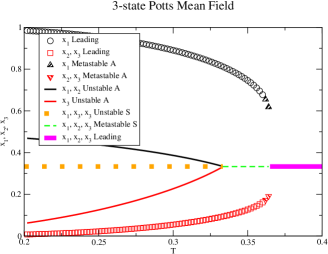
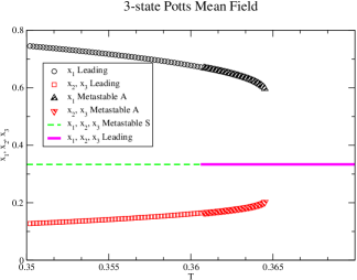
Eqs. (5)-(7) give rise to a well known phase transition scenario [1]: a second-order mean-field Ising phase transition sets up only for $q=2$, while for any $q\geq 3$ there is a first-order phase transition at the critical value (Fig. 1):

$$\beta^{(\mathrm{F.O.})}_{c}J=\frac{2(q-1)}{q-2}\log(q-1).$$ (8)

It is important to remind, however, that besides the solution giving rise to the first-order phase transition, and the trivial symmetric solution $x_{1}=\ldots=x_{q}=1/q$, which, in general, can be leading, metastable or unstable, for $q>2$ Eqs. (5)-(7) have also a non trivial unstable solution giving rise to a second order phase transition which sets in at the following critical point

$$\beta^{(\mathrm{S.O.~{}unstable})}_{c}J=q.$$ (9)

Eq. (9) establishes the temperature below which the symmetric solution is no longer metastable or stable. As we will see later, Eq. (9) has a stable counterpart when $J<0$ and a discrete-time dynamics is considered.

In Figs. (1) and (2) we plot all the possible solutions of Eqs. (7) and study their nature according to the free energy density (5). Note that a solution of Eqs. (4) is: leading if it is the absolute minimum for $f$; metastable if it is a local minimum for $f$; or unstable when is not a minimum for $f$ (i.e., at least one eigenvalue of the Hessian of the Landau free energy (5) is not positive).

Figure 1: (Color online) Magnetizations at equilibrium for the case $q=3$ and $J=1$. The first-order phase transition takes place at the critical temperature given by Eq. (8) which gives $T^{(\mathrm{F.O.})}_{c}=0.36067$, while the critical temperature of the unstable second-order phase transition is given by Eq. (9), which gives $T^{(\mathrm{S.O.~{}unstable})}_{c}=1/3$. In the figure: “Leading” stands for the thermodynamic stable state, i.e., having the lower free-energy, “Metastable” stands for the stable state having the higher free-energy, while “Unstable S” and “Unstable A” stand for the unstable states having the symmetry $x_{1}=x_{2}=x_{3}=1/3$ or not, respectively. The Leading states lie on the subspaces $x_{i_{1}}>x_{i_{2}}=x_{i_{3}}$ (in this figure only the case $x_{1}>x_{2}=x_{3}$ is shown), while the Unstable A states lie on the subspaces $x_{i_{1}}=x_{i_{2}}>x_{i_{3}}$ (in this figure only the case $x_{1}=x_{2}>x_{3}$ is shown), where $i_{1},i_{2},i_{3}$, is any permutation of the set of indices $\left\{1,2,3\right\}$ and $x_{i_{1}}+x_{i_{2}}+x_{i_{3}}=1$. Note that the asymptotic values of the magnetizations toward $T=0$ are $x_{i_{1}}=1,~{}x_{i_{2}}=x_{i_{3}}=0$ and $x_{i_{1}}=x_{i_{2}}=1/2,~{}x_{i_{3}}=0$, for the Leading and Unstable A states, respectively.

Figure 2: (Color online) Enlargement of Fig. (1). Notice, on this scale, the region of the metastable A (non symmetric) solution in a range of temperatures larger than $T^{(\mathrm{F.O.})}_{c}=0.3607$.

3 Equilibrium versus dynamics and the antiferromagnetic case

Above we have analyzed only the ferromagnetic case $J>0$. For the antiferromagnetic case $J<0$, it is possible to prove that the system remains in the trivial symmetric state [7]. By summarizing, at the Gibbs-Boltzmann equilibrium, for $q\geq 3$ the system undergoes a first-order phase transition only in the ferromagnetic case $J>0$, while in the antiferromagnetic case $J<0$ there is no phase transition.

A similar situation applies when one considers instead a dynamical approach, like the continuous-time Glauber dynamics [8]. The Glauber dynamics is a single spin-flip dynamics governed by the following master Eq.

$$\frac{dp(\sigma_{1},\ldots,\sigma_{N};t)}{\alpha dt}=$$

$$-\sum_{i}\sum_{\sigma^{{}^{\prime}}_{i}}w(\sigma_{i}\to\sigma^{{}^{\prime}}_{i})p(\sigma_{1},\ldots,\sigma_{N};t)+$$

$$\sum_{i}\sum_{\sigma^{{}^{\prime}}_{i}}w(\sigma^{{}^{\prime}}_{i}\to\sigma_{i})p(\sigma_{1},\ldots,\sigma_{i-1},\sigma^{{}^{\prime}}_{i},\sigma_{i+1},\ldots\sigma_{N};t),$$

where $p(\sigma_{1},\ldots,\sigma_{N};t)$ is the probability that the system is in the configuration $\sigma_{1},\ldots,\sigma_{N}$ at time $t$, $w(\sigma\to\sigma^{{}^{\prime}})$ are transition rate probabilities due to interaction with other spins, and $\alpha/q$ is the rate per unit time at which, due to the interaction with an heat reservoir, a free Potts spin makes transitions from either state to the other $q-1$. By imposing that, for $t\to\infty$, the system reaches equilibrium according to the Gibbs-Boltzmann probability $p(\sigma_{1},\ldots,\sigma_{N};t)\propto\exp(-\beta H)$, with $H$ given by Eq. (1), and by using the strong law of large numbers, it is easy to see that the transition rates must satisfy the following functional Eq. (also known as detailed-balance)

$$\sum_{\sigma}e^{\beta Jx_{\sigma}}w(\sigma\to\sigma^{{}^{\prime}})=e^{\beta Jx_{\sigma^{{}^{\prime}}}},$$ (11)

where, as in the previous Section, $x_{\sigma}$ is the probability to find any spin in the state $\sigma$ when $t\to\infty$. We will keep using the same symbol to indicate the probability to find any spin $\sigma_{i}$ in the state $\sigma$ also for finite $t$: $p(\sigma_{i}=\sigma;t)=x_{\sigma}(t)$. Taking into account the normalization condition $\sum_{\sigma^{{}^{\prime}}}w(\sigma\to\sigma^{{}^{\prime}})=1$, we will consider the following natural solution of Eq. (11) [10]

$$w(\sigma\to\sigma^{{}^{\prime}})=\frac{e^{\beta Jx_{\sigma^{{}^{\prime}}}}}{\sum_{\sigma^{{}^{\prime\prime}}}e^{\beta Jx_{\sigma^{{}^{\prime\prime}}}}}.$$ (12)

Rates (12) have the remarkable feature, typical of mean-field models, that they depend only on the final states. This fact allows us to immediately derive the dynamical Eqs. governing the evolution of the $x_{\sigma}(t)$’s (also known as reduced dynamics [8]). By plugging Eqs. (12) in (3) we get the following $q$-coupled (of which $q-1$ are independent) differential Eqs. of the order parameters $x_{\sigma}(t)$

$$\frac{dx_{\sigma}(t)}{\alpha dt}=-x_{\sigma}(t)+\frac{e^{\beta Jx_{\sigma}(t)}}{\sum_{\sigma^{\prime}}e^{\beta Jx_{\sigma^{\prime}}(t)}},$$ (13)

Eqs. (13) can be more simply derived also from the time-dependent Ginzburg-Landau Eqs. $dx_{\sigma}/dt\propto\partial f(\left\{x_{\sigma}^{\prime}\right\})/\partial x_{\sigma}$, as it has been done to study the ferromagnetic Potts model in the presence of an oscillating external field [11]. We here, however, wanted to start from a microscopic probabilistic approach. Of course, in the stationary limit $t\to\infty$, Eqs. (13) are equivalent to the self-consistent Eqs. (4). Furthermore, among the stationary solutions of Eqs. (13), the dynamically stable ones coincide with the minima of the Landau density free-energy at equilibrium (5). And this holds for both the cases $J>0$ and $J<0$. As a consequence, apart from an initial transient, the Potts model at Gibbs-Boltzmann equilibrium, or along the continuous Glauber dynamic, do not present a significant difference.

Note that, the lhs of Eqs. (13) and the rate $\alpha$, that determine how fast the system reaches equilibrium, are due to the interaction of the spins with the medium environment, e.g. heat, while the rhs of Eqs. (13) stems from the interactions of neighboring spins at a given $\beta$.

In the place of the above continuous-time dynamics, we introduce now a discrete-time dynamics taking place at the discrete times $t=0,1,2,\ldots,$ by the following Eqs.

$$\frac{x_{\sigma}(t+1)-x_{\sigma}(t)}{\alpha}=-x_{\sigma}(t)+\frac{e^{\beta Jx_{\sigma}}}{\sum_{\sigma^{\prime}}e^{\beta Jx_{\sigma^{\prime}}}}.$$ (14)

Eqs. (14) can be derived from a discrete-time master Eq. in close analogy to the continuous case, the difference being the assumption that we consider only discrete times and then finite difference probabilities. Furthermore, we need to work with global transition rate probabilities defined in the full $q^{N}$-dimensional space of the $N$ spins. More precisely, if we introduce the spin vector $\bm{\sigma}=(\sigma_{1},\ldots,\sigma_{N})$, and the associated probability vector $p(\bm{\sigma})$, instead of Eq. (3), we have

$$\frac{p(\bm{\sigma};t+1)-p(\bm{\sigma};t)}{\alpha}=-\sum_{\bm{\sigma}^{{}^{\prime}}}p(\bm{\sigma};t)W(\bm{\sigma}\to\bm{\sigma}^{{}^{\prime}})~{}~{}~{}~{}$$ (15)

$$+\sum_{\bm{\sigma}^{{}^{\prime}}}p(\bm{\sigma}^{{}^{\prime}};t)W(\bm{\sigma}^{{}^{\prime}}\to\bm{\sigma}),$$

where we have introduced the global transition rates in terms of the local weights (12): $W(\bm{\sigma}\to\bm{\sigma}^{{}^{\prime}})=\prod_{i=1}^{N}w(\sigma_{i}\to\sigma_{i}^{{}^{\prime}})$ As will be made clear later, for the model to be consistent, unlike the continuous case, we must impose the boundary $\alpha\leq 1$. The difference between Eqs. (13) and Eqs. (14) is that in Eqs. (13) the medium acts continuously in time, while in Eqs. (14) the medium acts only at discrete times and, between one time and the next one, the spins do not move (alternatively, we can can see the spin as frozen). Whereas only Eqs. (13) can represent some description of a system of physical particles each other interacting via a physical medium, Eqs. (14) can represent a system of agents which interact via, e.g., exchange of information taking place at discrete random times , as in fact occurs in the actual world, especially in social or economical contexts.

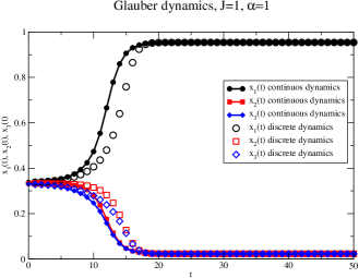
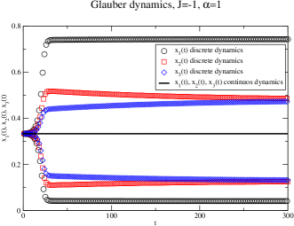
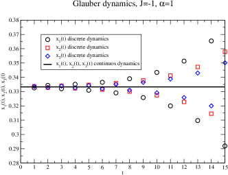
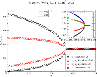
When $J>0$, the difference between Eqs. (13) and Eqs. (14) is not dramatic as, for $t\to\infty$, their solutions both tend to the the same $\alpha$-independent stable point-like stationary solutions of Eqs. (4) (see Fig. (3)). However, when $J<0$, for $t\to\infty$, whereas the solution of Eqs. (13) tends simply to the trivial symmetric one, the solution of Eqs. (14) tends, for $t\to\infty$, to a period-2 stable trajectory, i.e., the solution oscillates between two values (see Figs. (4) and (5)). Furthermore, with respect to the temperature, this solution undergoes a second-order phase transition belonging to the mean-field Ising universality class (as shown in Fig. (6), which represents the case $\alpha=1$). By changing $\alpha$, the critical behavior remains unchanged (and the curves are similar to those shown in Fig. (6)), while the critical temperature turns out to be a growing function of $\alpha$. Analytically, the mechanism can be understood and the critical temperature evaluated as follows. Let us look again for solutions in the form (6). From Eqs. (14) we have

$$x(t+1)=x(t)(1-\alpha)+\frac{\alpha}{1+(q-1)\exp\left(\beta J\frac{1-qx(t)}{q-1}\right)}.$$ (16)

Of course, the stationary solution of Eq. (16) that we get by imposing $x(t+1)=x(t)=x$, coincides with Eq. (7), so that, in particular, we already know that such stationary solutions do not undergo any phase transition when $J~{}<~{}0$. It is worth to remind that, in general, even tough a stationary Eq. has a solution, this does not necessary mean that the system reaches equilibrium. Eq. (16) for $J<0$ represents such a case: there exists the trivial stationary solution $x_{\sigma}=1/q$ but, nevertheless, the system never reaches equilibrium. Let us consider now the next time evolution. From Eq. (16) we have

$$x(t+2)=x(t)(1-\alpha)^{2}+\frac{\alpha(1-\alpha)}{1+(q-1)\exp\left(\beta J\frac{1-qx(t)}{q-1}\right)}$$

$$+\alpha\left[1+(q-1)\exp\left(\beta J\right.\right.$$

$$\times\left.\left.\frac{1-q\left[x(t)(1-\alpha)+\frac{\alpha}{1+(q-1)\exp\left(\beta J\frac{1-qx(t)}{q-1}\right)}\right]}{q-1}\right)\right]^{-1}$$ (17)

Let us analyze the stationary solutions of Eq. (3) that we get by imposing $x(t+2)=x(t)=x$, i.e., the period-2 stable trajectories. By writing $x=1/q-\epsilon$, and expanding Eq. (3) at the first order in $\epsilon$, it is not difficult to see that the solution $\epsilon=0$ becomes unstable when, for given $q$ and $\alpha$, the temperature satisfies the following Eq.

$$\alpha(\beta J)^{2}+2q(1-\alpha)\beta J-q^{2}(2-\alpha)=0.$$ (18)

As expected, when $J>0$, the only real root of Eq. (18) coincides with the critical (unstable) temperature of the equilibrium case Eq. (9). However, when $J<0$, the only real root of Eq. (18) is

$$\beta^{(\mathrm{S.O.})}_{c}J=q\left(1-\frac{2}{\alpha}\right),\quad\alpha\leq 1.$$ (19)

Eq. (19) says that the critical temperature is a growing function of $\alpha$. Notice that $\alpha=1$ returns the same value given by Eq. (9) with $J$ replaced by $|J|$ but, now, at low $T$, the states live on a subspace that oscillates between both the space of the states featured by the stable first-order transition that we had for $J>0$, and the space of the states of the unstable second-order transition that we had for $J>0$ (compare Figs. (1) and (6)).

Finally, by expanding Eq. (3) further, up to the third order in $\epsilon$, and by using Eq. (19), we obtain

$$A\tau\epsilon+(q-2)B\tau\epsilon^{2}+C\epsilon^{3}+\mathop{O}(\epsilon^{4})=0,$$ (20)

where $\tau=(T^{(\mathrm{S.O.})}_{c}-T)/T^{(\mathrm{S.O.})}_{c}$, and $A$, $B$, and $C$ are constants that do not depend on $\tau$. From (20) it follows that the critical behavior is Ising-like for any $\alpha$: $\epsilon\propto\tau^{1/2}$ (see enlargement of Fig. (6)). Notice that in the second term of the lhs of Eq. (20) we made explicit a dependence on the factor $q-2$ so that, the Ising case $q=2$, where the second term cancels exactly, is included as a special case.

We come now back to the necessary condition $\alpha\leq 1$. In fact, unlike the continuous case, in the lhs of the master Eq. (15) we have a difference of probabilities. Whereas the derivatives $dp/dt$ can take any real value, the finite difference of probabilities $p(t+1)-p(t)$ that appear in Eqs. (15), must lie in the interval [-1,1]. Or, in other words, we have to ensure that, given that $p(t)$ is a probability, $p(t+1)$ is also a probability. Note that, for any real $\alpha$, both Eqs. (3) or (15) give rise to normalized $p(\sigma_{1},\ldots,\sigma_{N};t)$’s at any $t$, but, in general, it may happen that the $p(t)$’s can take values outside the probability range $[0,1]$. Let us rewrite Eq. (15) in compact matrix notation:

$$\bm{p}(t+1)=\bm{p}(t)\left[\alpha\bm{W}+(1-\alpha)\bm{1}\right].$$ (21)

From Eq. (21) we see that the matrix appearing to the right hand side is a stochastic matrix (i.e. all the entries are positive and the rows are normalized to 1) when $\alpha<1$ and, as a consequence the Markov chain $\bm{p}(t)$ is a well defined probability.

Figure 3: (Color online) Continuous- and discrete-time Glauber dynamics for a 3-state Potts model with ferromagnetic coupling $J=1$ and $\alpha=1$. The continuous and discrete case are solutions of Eqs. (13) and (14), respectively, with initial conditions close to the symmetric solution: $x_{1}(0)=0.3369$, $x_{2}(0)=0.3331$, $x_{3}(0)=0.33$. The chosen temperature is $T/J=1/4$, which is lower than the first-order critical temperature of this case, $T^{(\mathrm{F.O.})}_{c}/J=0.3607$.

Figure 4: (Color online) Continuous- and discrete-time Glauber dynamics for a 3-state Potts model with anti-ferromagnetic coupling $J=-1$ and $\alpha=1$. The continuous and discrete case are the solutions of Eqs. (13) and (14), respectively, with initial conditions as in Fig. 3. The chosen temperature is $T/J=1/4$, which is lower than the critical temperature of this case, $T^{(\mathrm{S.O.})}_{c}/|J|=1/3$, where a second-order phase transition takes place. Note that the system never reaches point-like equilibrium (see Fig. (5)).

Figure 5: (Color online) Enlargement of Fig. 4. Notice, on this scale, the oscillating behavior of each component.

Figure 6: (Color online) Magnetizations of the period-2 attractor of Eqs. (14) for the case $q=3$, $J=-1$ and $\alpha=1$. Once reached the attractor (for large enough discrete times $t$), each component $x_{i}$ oscillates periodically taking the two values $x_{i}(2t)$ and $x_{i}(2t+1)$ (in this figure only the case $x_{1}>x_{2}=x_{3}$ for $t$ even, and $x_{1}<x_{2}=x_{3}$ for $t$ odd, are shown). Inset: enlargement around the transition point where, for $T\leq T^{(\mathrm{S.O.})}_{c}$, we plot also the matching functions $y(T)=1/3+1.35(T^{(\mathrm{S.O.})}_{c}-T)^{1/2}$ and $z(T)=1/3+0.65(T^{(\mathrm{S.O.})}_{c}-T)^{1/2}$, with $T^{(\mathrm{S.O.})}_{c}=1/3$, that confirm the Ising-like critical behavior.

4 Conclusions

We have shown that anti-ferromagnetic models that evolve along a discrete-time dynamics, as opposed to a continuous-time dynamics, reach period-2 stable trajectories where, after an initial transient, the order parameter oscillates between two values each of which undergoes a phase transition. Quite unexpectedly, the nature of such a phase transition is second-order, even though the only possible phase transitions of the Gibbs-Boltzmann equilibrium case were first-order. We have analyzed here the mean-field $q$-state Potts case in detail, but we believe this scenario being quite typical and robust with respect to the model definition. The results of our analysis shed some light to real-world models. Many real-world models, like social networks, population growths, economic networks, etc…, are in fact characterized by random interactions that take place not continuously, but only at certain discrete random times. Furthermore, a portion of these interactions are often unfriendly, i.e., anti-ferromagnetic. Therefore, at least at the mean-field level, and in the absence of quenched disorder, that would involve a glassy behavior [12], such real-world models are expected to reach a stable oscillating behavior and undergo a second-order phase transition for each component of the order parameter.