Branching processes with competition and generalized Ray Knight Theorem

Abstract

We consider a discrete model of population with interaction where the birth and death rates are non linear functions of the population size. After proceeding to renormalization of the model parameters, we obtain in the limit of large population that the population size evolves as a diffusion solution of the SDE

$$Z^{x}_{t}=x+\int_{0}^{t}f(Z^{x}_{s})ds+2\int_{0}^{t}\int_{0}^{Z^{x}_{s}}W(ds,du),$$

where $W(ds,du)$ is a time space white noise on $([0,\infty))^{2}$.
We give a Ray-Knight representation of this diffusion in terms of the local times of a reflected Brownian motion $H$ with a drift that depends upon the local time accumulated by $H$ at its current level, through the function $f^{\prime}/2$.

LATP-UMR 6632, CMI, Université de Provence, 39 rue F. Joliot Curie,
Marseille cedex 13, FRANCE.
email : mba@cmi.univ-mrs.fr ; pardoux@cmi.univ-mrs.fr   
  
  
.

Introduction

Consider a population evolving in continuous time with $m$ ancestors at time $t=0$, in which each individual, independently of the others, gives birth to children at a constant rate $\mu$, and dies after an exponential time with parameter $\lambda$. For each individual we superimpose additional birth and death rates due to interactions with others at a certain rate which depends upon the size of the total population. For instance, we might decide that each individual dies because of competition at a rate equal to $\gamma$ times the number of presently alive individuals in the population, which amounts to add a global death rate equal to $\gamma(X^{m}_{t})^{2}$, if $X^{m}_{t}$ denotes the total number of alive individuals at time $t$.

If we consider this population with $m=[Nx]$ ancestors at time $t=0$, weight each individual with the factor $1/N$, and choose $\mu_{N}=2N+\theta$, $\lambda_{N}=2N$ and $\gamma_{N}=\gamma/N$, then it is shown in Le, Pardoux and Wakolbinger [11] in the above particular case of a quadratic competition term that the “total population mass process” converges weakly to the solution of the Feller SDE with logistic drift

$$dZ^{x}_{t}=\left[\theta Z^{x}_{t}-\gamma(Z^{x}_{t})^{2}\right]dt+2\sqrt{Z^{x}_{t}}dW_{t},~{}Z^{x}_{0}=x.$$ (0.1)

The diffusion $Z^{x}$ is called Feller diffusion with logistic growth and models the evolution of the size of a large population with competition. In this model $\theta$ represent the supercritical branching parameter while $\gamma$ is the rate at which each individual is killed by any one of his contemporaneans. This model has been studied in Lambert [10], who shows in particular that its extinction time is finite almost surely.

We generalize the logistic model by replacing the quadratic function $\theta z-\gamma z^{2}$ by a more general nonlinear function $f$ of the population size. We then obtain in the continuous setting a diffusion which is the solution of the SDE

$$Z^{x}_{t} =x+\int_{0}^{t}f(Z^{x}_{s})ds+2\int_{0}^{t}\int_{0}^{Z^{x}_{s}}W(ds,du),$$ (0.2)

where the function $f$ satisfies the following hypothesis.
Hypothesis A: $f\in C(\mathbb{R}_{+};\mathbb{R})$, $f(0)=0$ and $\exists\beta\geq 0$ such that

$$f(x+y)-f(x)\leq\beta y\quad\forall x,y\geq 0.$$

The equation (0.2) has a unique strong solution (see [7]). Note that the hypothesis A implies that

$$\forall x\geq 0,f(x)\leq\beta x.$$

An equivalent way to write (0.2) is the following.

$$Z^{x}_{t}=x+\int_{0}^{t}f(Z^{x}_{s})ds+2\int_{0}^{t}\sqrt{Z^{x}_{s}}dW^{x}_{s},$$ (0.3)

where $W^{x}$ is a standard Brownian motion. However, the joint evolution of the various population sizes $\left\{Z^{x}_{t},t\geq 0\right\}$ corresponding to different initial population sizes $x$ would necessitate a complicated description of the joint law of the $\left\{W^{x}_{.},x\geq 0\right\}$. Whereas the formulation (0.2) due to Dawson, Li [7] with one unique space-time white noise $W$, describes exactly the joint evolution of $\left\{Z^{x}_{t},t\geq 0,x\geq 0\right\}$ which we have in mind. We call this diffusion the generalized Feller diffusion. In order to derive this continuous model, we first define a discrete model. For defining jointly the discrete model for all initial population sizes, we need as in [13] to impose a non symmetric competition rule between the individuals, which we will describe in section 1 below. We do a suitable renormalization of the parameters of the discrete model in order to obtain in section 2 a large population limit of our model which is a generalized Feller diffusion. Section 3 is devoted to give a Ray Knight representation for such a generalized Feller diffusion. The proof of this representation uses tools from stochastic analysis, in particular the “excursion filtration”, following an analogous proof of another generalized Ray Knight theorem in [12].

1 Discrete model with a general interaction

In this section we set up a discrete mass continuous time approximation of the generalized Feller diffusion. We consider a discrete model of population with interaction in which each individual, independently of the others, gives birth naturally at rate $\lambda$, dies naturally at rate $\mu$. Moreover, we suppose that each individual gives birth and dies because of interaction with others at rates which depend upon the current population size. Moreover, we exclude multiple births at any given time and we define the interaction rule through a function $f$ which satisfies hypothesis A.

In order to define our model jointly for all initial sizes, we need to introduce a non symmetric description of the effect of the interaction as in [3] and [11], but here we allow the interaction to be favorable to some individuals.

1.1 The model

We consider a continuous time $\mathbb{Z}_{+}$–valued population process $\{X^{m}_{t},\ t\geq 0\}$, which starts at time zero from $m$ ancestors who are arranged from left to right, and evolves in continuous time. The left/right order is passed on to their offsprings: the daughters are placed on the right of their mothers and if at a time $t$ the individual $i$ is located at the left of individual $j$, then all the offsprings of $i$ after time $t$ will be placed on the left of all the offsprings of $j$. Since we have excluded multiple births at any given time, this means that the forest of genealogical trees of the population is a planar forest of trees, where the ancestor of the population $X^{1}_{t}$ is placed on the far left, the ancestor of $X^{2}_{t}-X^{1}_{t}$ immediately on his right, etc… Moreover, we draw the genealogical trees in such a way that distinct branches never cross. This defines in a non–ambiguous way an order from left to right within the population alive at each time $t$. See Figure 1.

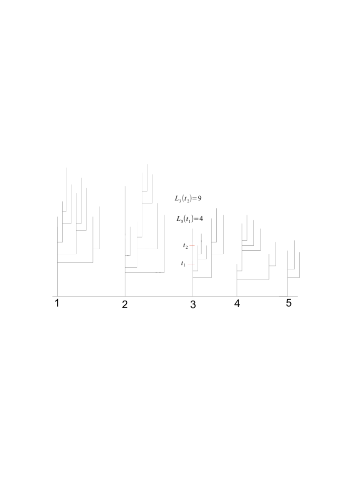
Figure 1: Planar forest with five ancestors

We decree that each individual feels the interaction with the others placed on his left but not with those on his right. Precisely, at any time $t$, the individual $i$ has an interaction death rate equal to $\left(f(\mathcal{L}_{i}(t)+1)-f(\mathcal{L}_{i}(t))\right)^{-}$ or an interaction birth rate equal to $\left(f(\mathcal{L}_{i}(t)+1)-f(\mathcal{L}_{i}(t))\right)^{+}$, where $\mathcal{L}_{i}(t)$ denotes the number of individuals alive at time $t$ who are located on the left of $i$ in the above planar picture. This means that the individual $i$ is under attack by the others located at his left if $f(\mathcal{L}_{i}(t)+1)-f(\mathcal{L}_{i}(t))<0$ while the interaction improve his fertility if $f(\mathcal{L}_{i}(t)+1)-f(\mathcal{L}_{i}(t))>0$. Of course, conditionally upon $\mathcal{L}_{i}(\cdot)$, the occurence of a “competition death event” or an “interaction birth event” for individual $i$ is independent of the other birth/death events and of what happens to the other individuals. In order to simplify our formulas, we suppose moreover that the first individual in the left/right order has a birth rate equal to $\lambda+f^{+}(1)$ and a death rate equal to $\mu+f^{-}(1)$.

The resulting total interaction death and birth rates endured by the population $X^{m}_{t}$ at time $t$ is then

$$\sum_{k=1}^{X^{m}_{t}}[(f(k)-f(k-1))^{+}-(f(k)-f(k-1)^{-}]=\sum_{k=1}^{X^{m}_{t}}(f(k)-f(k-1))=f(X^{m}_{t}).$$

As a result, $\{X^{m}_{t},\ t\geq 0\}$ is a continuous time $\mathbb{Z}_{+}$–valued Markov process, which evolves as follows. $X^{m}_{0}=m$. If $X^{m}_{t}=0$, then $X^{m}_{s}=0$ for all $s\geq t$. While at state $k\geq 1$, the process

$$X^{m}_{t}\text{ jumps to }\begin{cases}k+1,&\text{ at rate $\lambda k+\sum_{\ell=1}^{k}(f(\ell)-f(\ell-1))^{+}$};\\ k-1,&\text{ at rate $\mu k+\sum_{k=1}^{k}(f(\ell)-f(\ell-1))^{-}$}.\end{cases}$$

1.2 Coupling over ancestral population size

The above description specifies the joint evolution of all $\{X^{m}_{t},\ t\geq 0\}_{m\geq 1}$, or in other words of the two–parameter process $\{X^{m}_{t},\ t\geq 0,m\geq 1\}$. In the case of a linear function $f$, for each fixed $t>0$, $\{X^{m}_{t},\ m\geq 1\}$ is an independent increments process. In the case of a nonlinear function $f$, we believe that for $t$ fixed $\{X^{m}_{t},\ m\geq 1\}$ is not a Markov chain. That is to say, the conditional law of $X^{n+1}_{t}$ given $X^{n}_{t}$ differs from its conditional law given $(X^{1}_{t},X^{2}_{t},\ldots,X^{n}_{t})$. The intuitive reason for that is that the additional information carried by $(X^{1}_{t},X^{2}_{t},\ldots,X^{n-1}_{t})$ gives us a clue as to the fertility or the level of competition that the progeny of the $n+1$st ancestor had to beneficit or to suffer from, between time 0 and time $t$.

However, $\{X^{m}_{\cdot},\ m\geq 1\}$ is a Markov chain with values in the space $D([0,\infty);\mathbb{Z}_{+})$ of càdlàg functions from $[0,\infty)$ into $\mathbb{Z}_{+}$, which starts from 0 at $m=0$. Consequently, in order to describe the law of the whole process, that is of the two–parameter process $\{X^{m}_{t},\ t\geq 0,m\geq 1\}$, it suffices to describe the conditional law of $X^{n}_{\cdot}$, given $\{X^{n-1}_{\cdot}\}$. We now describe that conditional law for arbitrary $1\leq m<n$. Let $V^{m,n}_{t}:=X^{n}_{t}-X^{m}_{t}$, $t\geq 0$. Conditionally upon $\{X^{\ell}_{\cdot},\ \ell\leq m\}$, and given that $X^{m}_{t}=x(t)$, $t\geq 0$, $\{V^{m,n}_{t},\ t\geq 0\}$ is a $\mathbb{Z}_{+}$–valued time inhomogeneous Markov process starting from $V^{m,n}_{0}=n-m$, whose time–dependent infinitesimal generator $\{Q_{k,\ell}(t),\ k,\ell\in\mathbb{Z}_{+}\}$ is such that its off–diagonal terms are given by

$$Q_{0,\ell}(t) =0,\quad\forall\ell\geq 1,\quad\text{ and for any }k\geq 1,$$

$$Q_{k,k+1}(t) =\mu k+\sum_{\ell=1}^{k}(f(x(t)+\ell)-f(x(t)+\ell-1))^{+},$$

$$Q_{k,k-1}(t) =\lambda k+\sum_{\ell=1}^{k}(f(x(t)+\ell)-f(x(t)+\ell-1))^{-},$$

$$Q_{k,\ell}(t) =0,\quad\forall\ell\not\in\{k-1,k,k+1\}.$$

The reader can easily convince himself that this description of the conditional law of $\{X^{n}_{t}-X^{m}_{t},\ t\geq 0\}$, given $X^{m}_{\cdot}$ is prescribed by what we have said above, and that $\{X^{m}_{\cdot},\ m\geq 1\}$ is indeed a Markov chain.

Remark 1.1

Note that if the function $f$ is increasing on [0, $a$], $a>0$ and decreasing on $[a,\infty)$, the interaction improves the rate of fertility in a population whose size is smaller than $a$ but for large size the interaction amounts to competition within the population. This is reasonable because when the population is large, the limitation of resources implies competition within the population. For a positive interaction (for moderate population sizes) one can realize that an increase in the population size allows a more efficient organization of the society, with specalisation among its members, thes resulting in better food production, health care, etc… We are mainly interested in the model with interaction defined with functions $f$ such that $\lim_{x\to\infty}f(x)=-\infty.$ Note also that we could have generalized our model to the case $f(0)\geq 0$. $f(0)>0$ would mean an immigration flux. The reader can easily check that results in section 2 would still be valid in this case. However in Proposition 1.3 and in section 3.3 below, assumption $f(0)=0$ is crucial, since we need the population to get extinct in finite time $a.s.$.

1.3 The associated exploration process in the discrete model

The just described reproduction dynamics gives rise to a forest $\mathcal{F}^{m}$ of $m$ trees of descent, drawn into the plane as sketched in Figure 2. Note also that, with the above described construction, the $\left(\mathcal{F}^{m},m\geq 1\right)$, are coupled: the forest $\mathcal{F}^{m+1}$ has the same law as the forest $\mathcal{F}^{m}$ to which we add a new tree generated by an ancestor placed at the $(m+1)$st position. If the function $f$ tends to $-\infty$ and $m$ is large enough, the trees further to the right of the forest $\mathcal{F}^{m}$ have a tendency to stay smaller because of the competition : they are “under attack” from the trees to their left. From $\mathcal{F}^{m}$ we read off a continuous and piecewise linear $\mathbb{R}_{+}$-valued path $H^{m}=\left(H^{m}_{s}\right)$ (called the exploration process of $\mathcal{F}^{m}$) which is described as follows.

Starting from the initial time $s=0$ the process $H^{m}$ rises at speed $p$ until it hits the top of the first ancestor branch (this is the leaf marked with $D$ in Figure 2). There it turns and goes downwards, now at speed $-p$, until arriving at the next branch point (which is $B$ in Figure 2). From there it goes upwards into the (yet unexplored) next branch, and proceeds in a similar fashion until being back at height 0, which means that the exploration of the leftmost tree is completed. Then explore the next tree, and so on. See Figure 2.

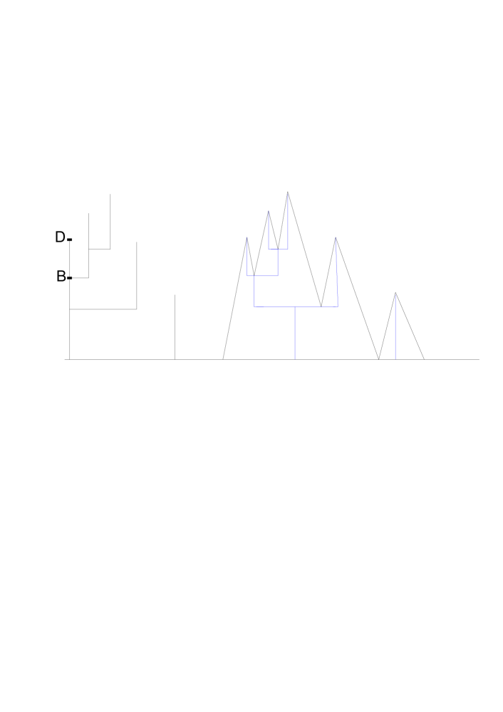
Figure 2: A forest with two trees and its exploration process.

We define the local time $L^{m}_{s}(t)$ accumulated by the process $H^{m}$ at level $t$ up to time $s$ by:

$$L^{m}_{s}(t)=\lim_{\epsilon\rightarrow 0}\frac{1}{\epsilon}\int_{0}^{s}1_{t\leq H^{m}_{r}<t+\epsilon}dr.$$

The process $H^{m}$ is piecewise linear, continuous with derivative $\pm p$ : at any time $s\geq 0$, the rate of appearance of minima (giving rise to new branches) is equal

$$p\mu+\left[f(\lfloor\frac{p}{2}L^{m}_{s}(H^{m}_{s})\rfloor+1)-f(\lfloor\frac{p}{2}L^{m}_{s}(H^{m}_{s})\rfloor)\right]^{+},$$

and the rate of appearance of maxima (describing deaths of branches) is equal to

$$p\lambda+\left[f(\lfloor\frac{p}{2}L^{m}_{s}(H^{m}_{s})\rfloor+1)-f(\lfloor\frac{p}{2}L^{m}_{s}(H^{m}_{s})\rfloor)\right]^{-}.$$

Let $S^{m}$ be the time needed in order to explore the forest $\mathcal{F}^{m}$. We have

$$S^{m}=\inf\{s>0;\frac{p}{2}L^{m}_{s}(0)\geq m\}.$$

Under the assumption that $S^{m}<\infty$ $a.s.$ for all $m\geq 1$, we have the following discrete Ray Knight representation (see Figure 3).

$$\left(X^{m}_{t},t\geq 0,m\geq 1\right)\equiv\left(\frac{p}{2}L^{m}_{S^{m}}(t),t\geq 0,m\geq 1\right).$$

Figure 3: Discrete Ray Knight representation.

1.4 Renormalized discrete model

Now we proceed to a renormalization of this model. For $x\in\mathbb{R}_{+}$ and $N\in\mathbb{N}$, we choose $m=\lfloor Nx\rfloor$, $\mu=2N$, $\lambda=2N$, we multiply $f$ by N and divide by $N$ the argument of the function $f$. We affect to each individual in the population a mass equal to $1/N$. Then the total mass process $Z^{N,x}$, which starts from $\frac{\lfloor Nx\rfloor}{N}$ at time $t=0$, is a Markov process whose evolution can be described as follows.
$Z^{N,x}$ jumps from $\frac{k}{N}$ to $\begin{cases}\frac{k+1}{N}\text{ at rate }2Nk+N\sum_{i=1}^{k}\left(f(\frac{i}{N})-f(\frac{i-1}{N})\right)^{+}\\ \frac{k+1}{N}\text{at rate }2Nk+N\sum_{i=1}^{k}\left((f(\frac{i}{N})-f(\frac{i-1}{N})\right)^{-},\end{cases}$
Clearly there exist two mutually independent standard Poisson processes $P_{1}$ and $P_{2}$ such that

$$Z^{N,x}_{t} =\frac{\lfloor Nx\rfloor}{N}+\frac{1}{N}P_{1}\left(\int_{0}^{t}\left(2N^{2}Z^{N,x}_{r}+N\sum_{i=1}^{NZ^{N,x}_{r}}(f(\frac{i}{N})-f(\frac{i-1}{N}))^{+}\right)dr\right)$$

$$-\frac{1}{N}P_{2}\left(\int_{0}^{t}\left(2N^{2}Z^{N,x}_{r}+N\sum_{i=1}^{NZ^{N,x}_{r}}(f(\frac{i}{N})-f(\frac{i-1}{N}))^{-}\right)dr\right).$$

Consequently there exists a local martingale $M^{N,x}$ such that

$$Z^{N,x}_{t}=\frac{\lfloor Nx\rfloor}{N}+\int_{0}^{t}f(Z^{N,x}_{r})dr+M^{N,x}_{t}.$$ (1.1)

Since $M^{N,x}$ is a purely discontinous local martingale, its quadratic variation $[M^{N,x}]$ is given by the sum of the squares of its jumps, i.e.

$$[M^{N,x}]_{t} =\frac{1}{N^{2}}\left[P_{1}\left(\int_{0}^{t}\left(2N^{2}Z^{N,x}_{r}+N\sum_{i=1}^{NZ^{N,x}_{r}}(f(\frac{i}{N})-f(\frac{i-1}{N}))^{+}\right)dr\right)\right.$$

$$\left.+P_{2}\left(\int_{0}^{t}\left(2N^{2}Z^{N,x}_{r}+N\sum_{i=1}^{NZ^{N,x}_{r}}(f(\frac{i}{N})-f(\frac{i-1}{N}))^{-}\right)dr\right)\right].$$ (1.2)

We deduce from (1.4) that the conditional quadratic variation $\langle M^{N,x}\rangle$ of $M^{N,x}$ is given by

$$\langle M^{N,x}\rangle_{t}=\int_{0}^{t}\left\{4Z^{N,x}_{r}+\frac{1}{N}||f||_{N,0,Z^{N,x}_{r}}\right\}dr,$$ (1.3)

where for any $z=\frac{k}{N}$, $z^{\prime}=\frac{k^{\prime}}{N}$, $k\in\mathbb{Z}_{+}$ such that  $k\leq k^{\prime}$,

$$||f||_{N,z,z^{\prime}}=\sum_{i=k+1}^{k^{\prime}}|f(\frac{i}{N})-f(\frac{i-1}{N})|.$$

Now we precise the law of the pair $\left(Z^{N,x},Z^{N,y}\right)$, for any $x,y\in\mathbb{R}_{+}$ such that $x\leq y$. Let $V^{N,x,y}:=Z^{N,y}-Z^{N,x}$, and consider the pair of process $\left(Z^{N,x},V^{N,x,y}\right)$, which starts from $\left(\frac{\lfloor Nx\rfloor}{N},\frac{\lfloor Ny\rfloor-\lfloor Nx\rfloor}{N}\right)$ at time $t=0$, and whose dynamic is described by: $\left(Z^{N,x},V^{N,x,y}\right)$ jumps
from $(\frac{i}{N},\frac{j}{N})$ to $\begin{cases}(\frac{i+1}{N},\frac{j}{N})\text{ at rate }2Ni+\sum_{k=1}^{i}(f(\frac{k}{N})-f(\frac{k-1}{N})^{+}\\ (\frac{i-1}{N},\frac{j}{N})\text{ at rate }2Ni+\sum_{k=1}^{i}(f(\frac{k}{N})-f(\frac{k-1}{N}))^{-}\\ (\frac{i}{N},\frac{j+1}{N})\text{ at rate }2Nj+\sum_{k=1}^{j}(f(\frac{i+k}{N})-f(\frac{i+k-1}{N})^{+}\\ (\frac{i}{N},\frac{j-1}{N})\text{ at rate }2Nj+\sum_{k=1}^{j}(f(\frac{i+k}{N})-f(\frac{i+k-1}{N})^{-}\end{cases}$.
The process $V^{N,x,y}$ can be expressed as follows.

$$V^{N,x,y}_{t}=\frac{\lfloor Ny\rfloor-\lfloor Nx\rfloor}{N}+\int_{0}^{t}\left[f(Z^{N,x}_{r}+V^{N,x,y}_{r})-f(Z^{N,x}_{r})\right]dr+M^{N,x,y}_{t},$$ (1.4)

where $M^{N,x,y}$ is a local martingale whose conditional quadratic variation $\langle M^{N,x,y}\rangle$ is given by

$$\langle M^{N,x,y}\rangle_{t}=\int_{0}^{t}\left\{4V^{N,x,y}_{r}+\frac{1}{N}||f||_{N,Z^{N,x}_{r},V^{N,x,y}+Z^{N,x}_{r}}\right\}dr.$$ (1.5)

Since $Z^{N,x}$ and $V^{N,x,y}$ never jump at the same time,

$$[M^{N,x},M^{N,x,y}]=0,\text{ hence }\langle M^{N,x},M^{N,x,y}\rangle=0,$$ (1.6)

which implies that the martingales $M^{N,x}$ and $M^{N,x,y}$ are orthogonal.

Consequently, $Z^{N,x}+V^{N,x,y}$ solves the SDE

$$Z^{N,x}_{t}+V^{N,x,y}_{t}= \frac{\lfloor Ny\rfloor}{N}+\int_{0}^{t}f(Z^{N,x}_{r}+V^{N,x,y}_{r})dr+\tilde{M}^{N,x,y}_{t}.$$

where $\tilde{M}^{N,x,y}$ is a local martingale with $\langle\tilde{M}^{N,x,y}\rangle$ given by

$$\langle\tilde{M}^{N,x,y}\rangle_{t} =\langle M^{N,x}\rangle_{t}+\langle M^{N,x,y}\rangle_{t}=\langle M^{N,x+y}\rangle_{t},\quad\forall t\geq 0.$$

We then deduce that for any $x,y\in\mathbb{R}_{+}$ such $x\leq y,$

$$Z^{N,x}+V^{N,x,y}\stackrel{{\scriptstyle(d)}}{{=}}Z^{N,y}.$$

In fact, we have that

$$V^{N,x,y}_{t} =\frac{\lfloor Ny\rfloor-\lfloor Nx\rfloor}{N}+\frac{1}{N}P^{1}\left(N\int_{0}^{t}\sum_{k=1}^{NV^{N,x,y}_{s}}\left(f(Z^{N,x}_{s}+\frac{k}{N})-f(Z^{N,x}_{s}+\frac{k}{N})\right)^{+}ds\right)$$

$$-\frac{1}{N}P^{2}\left(N\int_{0}^{t}\sum_{k=1}^{NV^{N,x,y}_{s}}\left(f(Z^{N,x}_{s}+\frac{k}{N})-f(Z^{N,x}_{s}+\frac{k}{N})\right)^{-}ds\right)$$

$$+\frac{1}{N}P^{3}\left(2N^{2}\int_{0}^{t}V^{N,x,y}_{s}ds\right)-\frac{1}{N}P^{4}\left(2N^{2}\int_{0}^{t}V^{N,x,y}_{s}ds\right),$$

where $P^{1}$, $P^{2}$, $P^{3}$ and $P^{4}$ are mutually independent standard Poisson processes which are all independent of $Z^{N,x}_{.}$. It follows that conditionally upon $\left\{Z^{N,x^{\prime}},x^{\prime}\leq x\right\}$, $M^{N,x,y}$ is a local martingale.

Remark 1.2

We can also proceed to the renormalisation of the exploration process to provide a discrete Ray Knight representation of the process $Z^{N,x}$. We choose the slope $p=2N$ and we denote by $H^{N}$ the exploration processes associated to the forest $\mathcal{F}^{N,x}$ of $\lfloor Nx\rfloor$ trees. Let $L^{N}_{s}(t)$ be the local time of the process $H^{N}$ at level $t$ up to time $s$. At any time $s$, the rate of minima of $H^{N}$ is equal to

$$4N^{2}+N\left[f(\frac{\lfloor NL^{N}_{s}(H^{N}_{s})\rfloor}{N}+1/N)-f(\frac{\lfloor NL^{N}_{s}(H^{N}_{s})\rfloor}{N})\right]^{+},$$

and the rate of maxima is equal to

$$4N^{2}+N\left[f(\frac{\lfloor NL^{N}_{s}(H^{N}_{s})\rfloor}{N}+1/N)-f(\frac{\lfloor NL^{N}_{s}(H^{N}_{s})\rfloor}{N})\right]^{-}.$$

Let $S^{N,x}$ be the time to explore the forest $\mathcal{F}^{N,x}$. We have that

$$S^{N,x}=\inf\{s>0;L^{N}_{s}(0)\geq\frac{\lfloor Nx\rfloor}{N}\}.$$

Under the assumption that $S^{N,x}<\infty$ $a.s.$ for all $x>0$, the discrete Ray Knight representation with the renormalization becomes:

$$\left(Z^{N,x}_{t},t\geq 0,x\geq 0\right)\equiv\left(L^{N}_{S^{N,x}}(t),t\geq 0,x\geq 0\right).$$

One could probably deduce from this discrete approximation the Ray Knight representation of the general Feller diffusion by a limiting argument, as it is done in [4] in the linear case and in [11] in the quadratic case. But in this work we use stochastic analysis tools for proving our extended Ray Knight theorem.

1.5 Continous model with a general competition

Given a space-time white noise $W(ds,du)$, we now define an $\mathbb{R}_{+}$–valued two–parameter stochastic process $\{Z^{x}_{t},\ t\geq 0,$ $x\geq 0\}$ which is such that for each fixed $x>0$, $\left\{Z^{x}_{t},t\geq 0\right\}$ is a continuous process, solution of the SDE (0.2). We have that for any $0<x<y$, $\{V^{x,y}_{t}:=Z^{y}_{t}-Z^{x}_{t},\ t\geq 0\}$ solves the SDE

$$V^{x,y}_{t}=y-x+\int_{0}^{t}\left[f(Z^{x}_{s}+V^{x,y}_{s})-f(Z^{x}_{s})\right]ds+2\int_{0}^{t}\int_{Z^{x}_{s}}^{Z^{x}_{s}+V^{x,y}_{s}}W(ds,du)$$ (1.7)

The process $V^{x,y}$ is nonnegative almost surely. We have that $\int_{0}^{t}\int_{0}^{Z^{x}_{s}}W(ds,du)$ and $\int_{0}^{t}\int_{Z^{x}_{s}}^{Z^{x}_{s}+V^{x,y}_{s}}W(ds,du)$ are orthogonal since

$$[0,Z^{x}_{s}]\cap(Z^{x}_{s},Z^{x}_{s}+V^{x,y}_{s}]=\emptyset,$$

and

$$\int_{0}^{t}\int_{0}^{Z^{x}_{s}}W(ds,du)+\int_{0}^{t}\int_{Z^{x}_{s}}^{Z^{x}_{s}+V^{x,y}_{s}}W(ds,du)=\int_{0}^{t}\int_{0}^{Z^{x}_{s}+V^{x,y}_{s}}W(ds,du)\text{ a.s.}$$

This implies that $Z^{y}=Z^{x}+V^{x,y}$ a.s. It follows that, for each $t\geq 0$, the process $\{Z^{x}_{t},x\geq 0\}$ is almost surely non decreasing and for $0\leq x<y$, the conditional law of $Z^{y}_{\cdot}$, given $\{Z^{x^{\prime}}_{t},x^{\prime}\leq x,t\geq 0\}$ and $Z^{x}_{t}=z(t)$, $t\geq 0$, is the law of the sum of $z$ plus the solution of (1.7) with $Z^{x}_{t}$ replaced by $z(t)$. Note that when $Z^{x}_{.}$ is replaced by a deterministic trajectory $z$, the solution of (1.7) is independent of $\{Z^{x^{\prime}}_{.},x^{\prime}<x\}$ . Hence the process $\{Z^{x}_{\cdot},\ x\geq 0\}$ is a Markov process with values in $C([0,\infty),\mathbb{R}_{+})$, the space of continuous functions from $[0,\infty)$ into $\mathbb{R}_{+}$, starting from $0$ at $x=0$. In the case $f$ linear, the increments of the mapping $x\to Z^{x}_{t}$ are independent, for each $t>0$.

For $x\geq 0$, define $T^{x}_{0}$ the extinction time of the process $Z^{x}$ by:

$$T^{x}_{0}=\inf\left\{t>0;Z^{x}_{t}=0\right\}.$$

For any $x\geq 0$, we call the process $Z^{x}$ subcritical if it goes extinct almost surely in finite time i.e if $T^{x}_{0}$ is finite almost surely. The assumption A implies that $\frac{f(x)}{x}$ is bounded. Let us introduce the notation

$$\Lambda(f):=\int_{1}^{\infty}\exp\left(-\frac{1}{2}\int_{1}^{u}\frac{f(r)}{r}dr\right)du.$$ (1.8)

We have the following Proposition.

Proposition 1.3

Suppose that $f$ satisfies hypothesis A. For any $x\geq 0$, $Z^{x}$ is subcritical if and only if $\Lambda(f)=\infty$. In particular we have:

• A sufficient condition for $\mathbb{P}\left(T^{x}_{0}<\infty\right)=1$ is: there exists $z_{0}\geq 1$ such that $f(z)\leq 2$, $\forall z\geq z_{0}$,

• A sufficient condition for $\mathbb{P}\left(T^{x}_{0}=\infty\right)>0$ is: there exists $z_{0}>1$ and $\delta>0$ such that $f(z)\geq 2+\delta$, $\forall$ $z\geq z_{0}$.

Proof:

Let $S\in C^{2}(\mathbb{R}_{+})$ and $0\leq a<x<b$. By Itô’s formula applied to the process $Z^{x}$ and the function $S$, we have that for any $t\geq 0$,

$$S(Z^{x}_{t})=S(x)+\int_{0}^{t}\left(S^{\prime}(Z^{x}_{s})f(Z^{x}_{s})+2S^{\prime\prime}(Z^{x}_{s})Z^{x}_{s}\right)ds+2\int_{0}^{t}S^{\prime}(Z^{x}_{s})\sqrt{Z^{x}_{s}}dW_{s}.$$ (1.9)

Let us denote by $\mathcal{A}$ the generator of $Z^{x}$. If we can find a strictly increasing function $S$ on the interval $[a,b]$ such that $\mathcal{A}S\equiv 0$, then the drift term in (1.9) vanishes and so $Z^{x}$ will be just a time changed Brownian motion in [$S(a)$, $S(b)$]. Such a function $S$ is called a scale function of the diffusion $Z^{x}$. We choose as scale function: for any $z\geq 0$,

$$S(z)=\int_{1}^{z}\exp\left(-\frac{1}{2}\int_{1}^{u}\frac{f(r)}{r}dr\right)du.$$

Let us denote by $T^{x}_{y}$ the random time at which $Z^{x}$ hits $y$ for the first time. We have for any $0\leq a<x<b$

$$\mathbb{P}(T^{x}_{a}<T^{x}_{b})=\frac{S(b)-S(x)}{S(b)-S(a)},\text{ and }\mathbb{P}(T^{x}_{a}<\infty)=\lim_{b\to\infty}\mathbb{P}(T^{x}_{a}<T^{x}_{b}).$$

If the function $S(z)$ tends to infinity as $z$ goes to infinity, then $\mathbb{P}(T^{x}_{a}<\infty)=1$. Otherwise $0<\mathbb{P}(T^{x}_{a}<\infty)<1$. From this we deduce that $Z^{x}$ goes extinct almost surely in finite time if and only if $\lim_{z\to\infty}S(z)=\infty$ i.e. if and only if $\Lambda(f)=\infty$. The rest of the Proposition is immediate.

 

2 Convergence as $N\to\infty$

The aim of this section is to prove the convergence in law as $N\to\infty$ of the two–parameter process $\{Z^{N,x}_{t},\ t\geq 0,x\geq 0\}$ defined in section 1.4 towards the process $\{Z^{x}_{t},\ t\geq 0,x\geq 0\}$ defined in section 1.5. We need to make precise the topology for which this convergence will hold. We note that the process $Z^{N,x}_{t}$ (resp. $Z^{x}_{t}$) is a Markov processes indexed by $x$, with values in the space of càdlàg (resp. continuous) functions of $t$ $D(([0,\infty);\mathbb{R}_{+})$ (resp. $C(([0,\infty);\mathbb{R}_{+})$). So it will be natural to consider a topology of functions of $x$, with values in functions of $t$.

For each fixed $x$, the process $t\to Z^{N,x}_{t}$ is càdlàg, constant between its jumps, with jumps of size $\pm N^{-1}$, while the limit process $t\to Z^{x}_{t}$ is continuous. On the other hand, both $Z^{N,x}_{t}$ and $Z^{x}_{t}$ are discontinuous as functions of $x$. $x\to Z^{x}_{\cdot}$ has countably many jumps on any compact interval, but the mapping $x\to\{Z^{x}_{t},\ t\geq\epsilon\}$, where $\epsilon>0$ is arbitrary, has finitely many jumps on any compact interval, and it is constant between its jumps. Recall that $D([0,\infty);\mathbb{R}_{+})$ equipped with the distance $d^{0}_{\infty}$ defined by $(16.4)$ in [5] is separable and complete, see Theorem $16.3$ in [5]. We have the following statement

Theorem 2.1

Suppose that the Hypothesis $\bf{A}$ is satisfied. Then as $N\to\infty$,

$$\{Z^{N,x}_{t},\ t\geq 0,x\geq 0\}\Rightarrow\{Z^{x}_{t},\ t\geq 0,x\geq 0\}$$

in $D([0,\infty);D([0,\infty);\mathbb{R}_{+}))$, equipped with the Skohorod topology of the space of càdlàg functions of $x$, with values in the Polish space $D([0,\infty);\mathbb{R}_{+})$ equipped with the metric $d^{0}_{\infty}$.

Proof of the theorem

To prove the theorem, we first show that for fixed $x\geq 0$ the sequence $\left\{Z^{N,x},~{}N\geq 0\right\}$ is tight in $D([0,\infty);\mathbb{R}_{+})$.

2.1 Tightness of $Z^{N,x}$

For this end, we first establish a few lemmas.

Lemma 2.2

For all $T>0$, $x\geq 0$, there exist a constant $C_{0}>0$ such that for all $N\geq 1$,

$$\sup_{0\leq t\leq T}\mathbb{E}\left(Z^{N,x}_{t}\right)\leq C_{0}.$$

Moreover, for all $t\geq 0$, $N\geq 1$,

$$\mathbb{E}\left(-\int_{0}^{t}f(Z^{N,x}_{r})dr\right)\leq x.$$

Proof: Let $\left(\tau_{n},n\geq 0\right)$ be a sequence of stopping times such that $\tau_{n}$ tends to infinity as $n$ goes to infinity and for any $n$, $\left(M^{N,x}_{t\wedge\tau_{n}},t\geq 0\right)$ is a martingale and $Z^{N,x}_{t\wedge\tau_{n}}\leq n$. Taking the expectation on both sides of equation (1.1) at time $t\wedge\tau_{n}$, we obtain

$$\mathbb{E}\left(Z^{N,x}_{t\wedge\tau_{n}}\right)=\frac{\lfloor Nx\rfloor}{N}+\mathbb{E}\left(\int_{0}^{t\wedge\tau_{n}}f(Z^{N,x}_{r})dr\right).$$ (2.1)

It follows from the hypothesis A on $f$ that

$$\mathbb{E}\left(Z^{N,x}_{t\wedge\tau_{n}}\right)\leq\frac{\lfloor Nx\rfloor}{N}+\beta\int_{0}^{t}\mathbb{E}(Z^{N,x}_{r\wedge\tau_{n}})dr$$

From Gronwall and Fatou Lemmas, we deduce that there exists a constant $C_{0}>0$ which depends only upon $x$ and $T$ such that

$$\sup_{N\geq 1}\sup_{0\leq t\leq T}\mathbb{E}\left(Z^{N,x}_{t}\right)\leq C_{0}.$$

From (2.1), we deduce that

$$-\mathbb{E}\left(\int_{0}^{t\wedge\tau_{n}}f(Z^{N,x}_{r})dr\right)\leq\frac{\lfloor Nx\rfloor}{N}.$$

Since $-f(Z^{N,x}_{r})\geq-\beta Z^{N,x}_{r}$ , the second statement follows using Fatou’s Lemma and the first statement.  

We now have the following lemma.

Lemma 2.3

For all $T>0$, $x\geq 0$, there exists a constant $C_{1}>0$ such that :

$$\sup_{N\geq 1}\mathbb{E}\left(\langle M^{N,x}\rangle_{T}\right)\leq C_{1}.$$

Proof: For any $N\geq 1$ and $k,k^{\prime}\in\mathbb{Z}_{+}$ such that $k\leq k^{\prime}$, we set $z=\frac{k}{N}$ and $z^{\prime}=\frac{k^{\prime}}{N}$. We deduce from hypothesis A on $f$ that

$$||f||_{N,z,z^{\prime}} =\sum_{i=k+1}^{k^{\prime}}\left\{\left(f(\frac{i}{N})-f(\frac{i-1}{N})\right)^{+}+\left(f(\frac{i}{N})-f(\frac{i-1}{N})\right)^{-}\right\}$$

$$=\sum_{i=k+1}^{k^{\prime}}\left\{2\left(f(\frac{i}{N})-f(\frac{i-1}{N})\right)^{+}-\left(f(\frac{i}{N})-f(\frac{i-1}{N})\right)\right\}.$$

Consequentely,

$$||f||_{N,z,z^{\prime}}\leq 2\beta(z^{\prime}-z)+f(z)-f(z^{\prime}).$$ (2.2)

We deduce from (2.2), (1.3) and Lemma 2.2 that

$$\mathbb{E}\left(\langle M^{N,x}\rangle_{T}\right) \leq\int_{0}^{T}\left\{(4+\frac{2\beta}{N})\mathbb{E}(Z^{N,x}_{r})-\frac{1}{N}\mathbb{E}\left(f(Z^{N,x}_{r}\right)\right\}dr$$

$$\leq(4+\frac{2\beta}{N})C_{0}T+\frac{x}{N}.$$

Hence the lemma.  

It follows from this that $M^{N,x}$ is in fact a square integrable martingale. We also have

Lemma 2.4

For all $T>0$, $x\geq 0$, there exist two constants $C_{2},C_{3}>0$ such that  :

$$\sup_{N\geq 1}\sup_{0\leq t\leq T}\mathbb{E}\left(Z^{N,x}_{t}\right)^{2} \leq C_{2},$$

$$\sup_{N\geq 1}\sup_{0\leq t\leq T}\mathbb{E}\left(-\int_{0}^{t}Z^{N,x}_{r}f(Z^{N,x}_{r})dr\right) \leq C_{3}.$$

Proof: We deduce from (1.1) and Itô’s formula that

$$\left(Z^{N,x}_{t}\right)^{2}=\left(\frac{\lfloor Nx\rfloor}{N}\right)^{2}+2\int_{0}^{t}Z^{N,x}_{r}f(Z^{N,x}_{r})dr+\langle M^{N,x}\rangle_{t}+M^{N,x,(2)}_{t},$$ (2.3)

where $M^{N,x,(2)}$ is a local martingale. Let $\left(\sigma_{n},n\geq 1\right)$ be a sequence of stopping times such that $\lim_{n\to\infty}\sigma_{n}=+\infty$ and for each $n\geq 1$, $\left(M^{N,x,(2)}_{t\wedge\sigma_{n}},t\geq 0\right)$ is a martingale. Taking the expectation on the both sides of (2.3) at time $t\wedge\sigma_{n}$ and using hypothesis A, Lemma 2.3, Gronwall and Fatou lemmas we obtain that for all $T>0$, there exists a constant $C_{2}>0$ such that :

$$\sup_{N\geq 1}\sup_{0\leq t\leq T}\mathbb{E}\left(Z^{N,x}_{t}\right)^{2}dr\leq C_{2}.$$

We also have that

$$2\mathbb{E}\left(-\int_{0}^{t\wedge\sigma_{n}}Z^{N,x}_{r}f(Z^{N,x}_{r})dr\right)\leq\left(\frac{\lfloor Nx\rfloor}{N}\right)^{2}+C_{1}$$

From Hypothesis A, we have $-Z^{N,x}_{r}f(Z^{N,x}_{r})\geq-\beta(Z^{N,x}_{r})^{2}$. The result now follows from Fatou’s Lemma.  

We want to check tightness of the sequence $\left\{Z^{N,x},~{}N\geq 0\right\}$ using Aldous’ criterion. Let $\left\{\tau_{N},~{}N\geq 1\right\}$ be a sequence of stopping time in $[0,T]$. We deduce from Lemma 2.4

Proposition 2.5

For any $T>0$ and $\eta$, $\epsilon>0$, there exists $\delta>0$ such that

$$\sup_{N\geq 1}\sup_{0\leq\theta\leq\delta}\mathbb{P}\left(\left|\int_{\tau_{N}}^{(\tau_{N}+\theta)\wedge T}f(Z^{N,x}_{r})dr\right|\geq\eta\right)\leq\epsilon.$$

Proof: Let $c$ be a non negative constant. We have

$$\left|\int_{\tau_{N}}^{(\tau_{N}+\theta)\wedge T}f(Z^{N,x}_{r})dr\right| \leq\sup_{0\leq r\leq c}|f(r)|\delta+\int_{\tau_{N}}^{\tau_{N}+\theta}{\bf 1}_{\{Z^{N,x}_{r}>c\}}|f(Z^{N,x}_{r})|dr$$

But

$$\int_{\tau_{N}}^{\tau_{N}+\theta}{\bf 1}_{\{Z^{N,x}_{r}>c\}}|f(Z^{N,x}_{r})|dr \leq c^{-1}\int_{0}^{T}Z^{N,x}_{r}\left(f^{+}(Z^{N,x}_{r})+f^{-}(Z^{N,x}_{r})\right)dr$$

$$\leq c^{-1}\int_{0}^{T}\left(2Z^{N,x}_{r}f^{+}(Z^{N,x}_{r})-Z^{N,x}_{r}f(Z^{N,x}_{r})\right)dr$$

$$\leq c^{-1}\int_{0}^{T}\left(2\beta(Z^{N,x}_{r})^{2}-Z^{N,x}_{r}f(Z^{N,x}_{r})\right)dr.$$

From this and Lemma 2.4, we deduce that $\forall$ $N\geq 1$

$$\sup_{0\leq\theta\leq\delta}\mathbb{P}\left(\Big{|}\int_{\tau_{N}}^{(\tau_{N}+\theta)\wedge T}f(Z^{N,x}_{r})dr\Big{|}\geq\eta\right) \leq\eta^{-1}\mathbb{E}\left(\left|\int_{\tau_{N}}^{(\tau_{N}+\theta)\wedge T}f(Z^{N,x}_{r})dr\right|\right)$$

$$\leq\sup_{0\leq r\leq c}\frac{|f(z)|\delta}{\eta}+\frac{A}{c\eta},$$

with $A=2\beta C_{2}T+C_{3}$. The result follows by choosing $c=2A/\epsilon\eta$, and then $\delta=\epsilon\eta/2\sup_{0\leq r\leq c}|f(z)|$.  

From Proposition 2.5, the Lebesgue integral term in the right hand side of (1.1) satisfies Aldou’s condition $[A]$, see [1]. The same Proposition, Lemma 2.2, (1.3) and (2.2) imply that $<M^{N,x}>$ satisfies the same condition, hence so does $M^{N,x}$, according to Rebolledo’s theorem, see [9]. Since all jumps are of size $\frac{1}{N}$, tightness follows. We have proved

Proposition 2.6

For any fixed $x\geq 0$, the sequence of processes $\left\{Z^{N,x},~{}N\geq 1\right\}$ is tight in $D\left([0,\infty);\mathbb{R}_{+}\right)$.

We deduce from Proposition 2.6 the following Corollary.

Corollary 2.7

For any $0\leq x<y$ the sequence of processes $\left\{V^{N,x,y},~{}N\geq 1\right\}$ is tight in $D\left([0,\infty);\mathbb{R}_{+}\right)$

Proof: For any $x$ fixed the process $Z^{N,x}$ has jumps equal to $\pm\frac{1}{N}$ which tends to zero as $N\to\infty$. It follows from that and equation (1.1) that any weak limit of a converging subsequence of $Z^{N,x}$ is continuous and is the unique weak solution of equation (0.2). We deduce that for any $x,y\geq 0$, the sequence $\left\{Z^{N,y}-Z^{N,x},N\geq 1\right\}$ is tight since $\left\{Z^{N,x},N\geq 1\right\}$ and$\left\{Z^{N,y},N\geq 1\right\}$ are tight and both have a continuous limit as $N\to\infty$.  

2.2 Proof of Theorem 2.1

From Theorem 13.5 in [5], Theorem 2.1 follows from the two next Propositions

Proposition 2.8

For any $n\in\mathbb{N}$, $0\leq x_{1}<x_{2}<\cdots<x_{n}$,

$$\left(Z^{N,x_{1}},Z^{N,x_{2}},\cdots,Z^{N,x_{n}}\right)\Rightarrow\left(Z^{x_{1}},Z^{x_{2}},\cdots,Z^{x_{n}}\right)$$

as $N\to\infty$, for the topology of locally uniform convergence in $t$.

Proof: We prove the statement in the case $n=2$ only. The general statement can be proved in a very similar way. For $0\leq x_{1}<x_{2}$, we consider the process $\left(Z^{N,x_{1}},V^{N,x_{1},x_{2}}\right)$, using the notations from section 1. The argument preceding the statement of Proposition 2.6 implies that the sequences of martingales $M^{N,x_{1}}$ and $M^{N,x_{1},x_{2}}$ are tight. Hence
$\left(Z^{N,x_{1}},V^{N,x_{1},x_{2}},M^{N,x_{1}},M^{N,x_{1},x_{2}}\right)$ is tight. Thanks to (1.1), (1.4), (1.3), (1.5) and (1.6), any converging subsequence of
$\left\{Z^{N,x_{1}},V^{N,x_{1},x_{2}},M^{N,x_{1}},M^{N,x_{1},x_{2}},N\geq 1\right\}$ has a weak limit
$\left(Z^{x_{1}},V^{x_{1},x_{2}},M^{x_{1}},M^{x_{1},x_{2}}\right)$ which satisfies

$$Z^{x_{1}}_{t} =x_{1}+\int_{0}^{t}f(Z^{x_{1}}_{s})ds+M^{x_{1}}_{t}$$

$$V^{x_{1},x_{2}}_{t} =x_{2}-x_{1}+\int_{0}^{t}f\left[f(Z^{x_{1}}_{s}+V^{x_{1},x_{2}}_{s})-f(Z^{x_{1}}_{s})\right]ds+M^{x_{1},x_{2}}_{t},$$

where the continuous martingales $M^{x_{1}}$ and $M^{x_{1},x_{2}}$ satisfy

$$\langle M^{x}\rangle_{t}=4\int_{0}^{t}Z^{x_{1}}_{s}ds,~{}\langle M^{x_{1},x_{2}}\rangle_{t}=4\int_{0}^{t}V^{x_{1},x_{2}}_{s}ds,~{}\langle M^{x_{1}},M^{x_{1},x_{2}}\rangle_{t}=0.$$

This implies that the pair $\left(Z^{x_{1}},V^{x_{1},x_{2}}\right)$ is a weak solution of the system of SDEs (0.2) and (1.7), driven by the same space-time white noise. The result follows from the uniqueness of the system, see [7].  

Proposition 2.9

There exists a constant $C$, which depends only upon $\theta$ and $T$, such that for any $0\leq x<y<z$, which are such that $y-x\leq 1$, $z-y\leq 1$,

$$\mathbb{E}\left[\sup_{0\leq t\leq T}|Z^{N,y}_{t}-Z^{N,x}_{t}|^{2}\times\sup_{0\leq t\leq T}|Z^{N,z}_{t}-Z^{N,y}_{t}|^{2}\right]\leq C|z-x|^{2}.$$

We first prove the

Lemma 2.10

For any $0\leq x<y$, we have

$$\sup_{0\leq t\leq T}\mathbb{E}\left(Z^{N,y}_{t}-Z^{N,x}_{t}\right)=\sup_{0\leq t\leq T}\mathbb{E}(V^{N,x,y}_{t})\leq\left(\frac{\lfloor Ny\rfloor}{N}-\frac{\lfloor Nx\rfloor}{N}\right)e^{\beta T},$$

Proof: Let $\left(\sigma_{n},n\geq 0\right)$ be a sequence of stopping times such that $\lim_{n\to\infty}\sigma_{n}=+\infty$ and $\left(M^{N,x,y}_{t\wedge\sigma_{n}}\right)$ is a martingale. Taking the expectation on the both sides of (1.4) at time $t\wedge\sigma_{n}$ we obtain that

$$\mathbb{E}(V^{N,x,y}_{t\wedge\sigma_{n}})\leq\left(\frac{\lfloor Ny\rfloor}{N}-\frac{\lfloor Nx\rfloor}{N}\right)+\beta\int_{0}^{t}\mathbb{E}(V^{N,x,y}_{r\wedge\sigma_{n}})dr$$ (2.4)

Using Gronwall and Fatou lemmas, we obtain that

$$\sup_{0\leq t\leq T}\mathbb{E}(V^{N,x,y}_{t})\leq\left(\frac{\lfloor Ny\rfloor}{N}-\frac{\lfloor Nx\rfloor}{N}\right)e^{\beta T}.$$

 

Proof of Proposition 2.9 Using equation (1.4), a stopping time argument as above, Lemma 2.10 and Fatou’s lemma, where we take advantage of the inequality $f(Z^{N,x}_{r})-f(Z^{N,x}_{r}+V^{N,x,y}_{r})\geq-\beta V^{N,x,y}_{r}$, we deduce that

$$\mathbb{E}\left(\int_{0}^{t}\left[f(Z^{N,x}_{r})-f(Z^{N,x}_{r}+V^{N,x,y}_{r})\right]dr\right)\leq\frac{\lfloor Ny\rfloor}{N}-\frac{\lfloor Ny\rfloor}{N}.$$ (2.5)

We now deduce from (1.5), Lemma 2.10, inequalities (2.5) and (2.2) that for each $t>0$, there exists a constant $C(t)>0$ such that

$$\mathbb{E}\left(\langle M^{N,x,y}\rangle_{t}\right)\leq C(t)\left(\frac{\lfloor Ny\rfloor}{N}-\frac{\lfloor Ny\rfloor}{N}\right).$$ (2.6)

This implies that $M^{N,x,y}$ is in fact a square integrable martingale. For any $0\leq x<y<z$, we have $Z^{N,z}_{t}-Z^{N,y}_{t}=V^{N,y,z}_{t}$ and $Z^{N,y}_{t}-Z^{N,x}_{t}=V^{N,x,y}_{t}$ for any $t\geq 0$. On the other hand we deduce from (1.4) and the hypothesis $\bf{A}$

$$\sup_{0\leq t\leq T}(V^{N,x,y}_{t})^{2} \leq 3\left(\frac{\lfloor Ny\rfloor}{N}-\frac{\lfloor Nx\rfloor}{N}\right)^{2}+3\beta^{2}T\int_{0}^{T}\sup_{0\leq s\leq r}(V^{N,x,y}_{s})^{2}dr$$

$$+3\sup_{0\leq t\leq T}\left(M^{N,x,y}_{t}\right)^{2},$$

$$\sup_{0\leq t\leq T}(V^{N,y,z}_{t})^{2} \leq 3\left(\frac{\lfloor Nz\rfloor}{N}-\frac{\lfloor Ny\rfloor}{N}\right)^{2}+3\beta^{2}T\int_{0}^{t}\sup_{0\leq s\leq r}(V^{N,y,z}_{s})^{2}dr$$

$$+3\sup_{0\leq t\leq T}\left(M^{N,y,z}_{t}\right)^{2}.$$

Now let $\mathcal{G}^{x,y}:=\sigma\left(Z^{N,x}_{t},Z^{N,y}_{t},t\geq 0\right)$ be the filtration generated by $Z^{N,x}$ and $Z^{N,y}$. It is clear that for any $t$, $V^{N,x,y}_{t}$ is measurable with respect to $\mathcal{G}^{x,y}$. We then have

$$\mathbb{E}\left[\sup_{0\leq t\leq T}|V^{N,x,y}_{t}|^{2}\times\sup_{0\leq t\leq T}|V^{N,y,z}_{t}|^{2}\right]=\mathbb{E}\left[\sup_{0\leq t\leq T}|V^{N,x,y}_{t}|^{2}\mathbb{E}\left(\sup_{0\leq t\leq T}|V^{N,y,z}_{t}|^{2}|\mathcal{G}^{x,y}\right)\right].$$

Conditionally upon $Z^{N,x}$ and $Z^{N,y}=u(.)$, $V^{N,y,z}$ solves the following SDE

$$V^{N,y,z}_{t}=\frac{\lfloor Nz\rfloor-\lfloor Ny\rfloor}{N}+\int_{0}^{t}\left[f(V^{N,y,z}_{r}+u(r))-f(u(r))\right]dr+M^{N,y,z}_{t},$$

where $M^{N,y,z}$ is a martingale conditionally upon $\mathcal{G}^{x,y}$, hence the arguments used in Lemma 2.10 lead to

$$\sup_{0\leq t\leq T}\mathbb{E}\left(V^{N,y,z}_{t}|\mathcal{G}^{x,y}\right)\leq\left(\frac{\lfloor Nz\rfloor}{N}-\frac{\lfloor Ny\rfloor}{N}\right)e^{\beta T},$$

and those used to prove (2.5) yield

$$\mathbb{E}\left(\int_{0}^{t}f(Z^{N,y}_{r})-f(Z^{N,y}_{r}+V^{N,y,z}_{r})dr|\mathcal{G}^{x,y}\right)\leq\frac{\lfloor Nz\rfloor}{N}-\frac{\lfloor Ny\rfloor}{N}.$$

From this we deduce (see the proof of (2.6)) that

$$\mathbb{E}\left(\langle M^{N,y,z}\rangle_{t}|\mathcal{G}^{x,y}\right)\leq C(t)\left(\frac{\lfloor Nz\rfloor}{N}-\frac{\lfloor Ny\rfloor}{N}\right).$$

From Doobs’s inequality we have

$$\mathbb{E}\left(\sup_{0\leq t\leq T}|M^{N,y,z}_{t}|^{2}|\mathcal{G}^{x,y}\right) =\mathbb{E}\left(\langle M^{N,y,z}\rangle_{T}|\mathcal{G}^{x,y}\right)$$

$$\leq C(T)\left(\frac{\lfloor Nz\rfloor}{N}-\frac{\lfloor Ny\rfloor}{N}\right).$$

Since $0<z-y<1$, we deduce that

$$\mathbb{E}\left(\sup_{0\leq t\leq T}|V^{N,y,z}_{t}|^{2}|\mathcal{G}^{x,y}\right) \leq 3(1+C(T))\left(\frac{\lfloor Nz\rfloor}{N}-\frac{\lfloor Ny\rfloor}{N}\right)$$

$$+3\beta^{2}T\int_{0}^{T}\mathbb{E}\left(\sup_{0\leq s\leq r}(V^{N,y,z}_{s})^{2}|\mathcal{G}^{x,y}\right)dr,$$

From this and Gronwall’s lemma we deduce that there exists a constant $K_{1}>0$ such that

$$\mathbb{E}\left(\sup_{0\leq t\leq T}|V^{N,y,z}_{t}|^{2}|\mathcal{G}^{x,y}\right)\leq K_{1}\left(\frac{\lfloor Nz\rfloor}{N}-\frac{\lfloor Ny\rfloor}{N}\right).$$ (2.7)

Similary we have

$$\mathbb{E}\left[\sup_{0\leq t\leq T}\left(V^{N,x,y}_{s}\right)^{2}\right]\leq K_{1}\left(\frac{\lfloor Ny\rfloor}{N}-\frac{\lfloor Nx\rfloor}{N}\right),$$

Since $0\leq y-x<z-x$ and $0\leq z-y<z-x$, we deduce that

$$\mathbb{E}\left[\sup_{0\leq t\leq T}|V^{N,x,y}_{t}|^{2}\times\sup_{0\leq t\leq T}|V^{N,y,z}_{t}|^{2}\right]\leq K_{1}^{2}\left(\frac{\lfloor Nz\rfloor}{N}-\frac{\lfloor Nx\rfloor}{N}\right)^{2},$$

hence the result.

Proof of Theorem 2.1 We now show that for any $T>0$,

$$\{Z^{N,x}_{t},\ 0\leq t\leq T,\ x\geq 0\}\Rightarrow\{Z^{x}_{t},\ 0\leq t\leq T,\ x\geq 0\}$$

in $D([0,\infty);D([0,T],\mathbb{R}_{+}))$. From Theorems 13.1 and 16.8 in [5], since from Proposition 2.8, for all $n\geq 1$, $0<x_{1}<\cdots<x_{n}$,

$$(Z^{N,x_{1}}_{\cdot},\ldots,Z^{N,x_{n}}_{\cdot})\Rightarrow(Z^{x_{1}}_{\cdot},\ldots,Z^{x_{n}}_{\cdot})$$

in $D([0,T];\mathbb{R}^{n})$, it suffices to show that for all $\bar{x}>0$, $\epsilon$, $\eta>0$, there exists $N_{0}\geq 1$ and $\delta>0$ such that for all $N\geq N_{0}$,

$$\mathbb{P}(w_{\bar{x},\delta}(Z^{N})\geq\epsilon)\leq\eta,$$ (2.8)

where for a function $(x,t)\to z(x,t)$

$$w_{\bar{x},\delta}(z)=\sup_{0\leq x_{1}\leq x\leq x_{2}\leq\bar{x},x_{2}-x_{1}\leq\delta}\inf\left\{\|z(x,\cdot)-z(x_{1},\cdot)\|,\|z(x_{2},\cdot)-z(x,\cdot)\|\right\},$$

with the notation $\|z(x,\cdot)\|=\sup_{0\leq t\leq T}|z(x,t)|$. But from the proof of Theorem 13.5 in [5], (2.8) for $Z^{N}$ follows from Proposition 2.9

3 Ray Knight representation of a general Feller diffusion

In this section we establish a Ray-Knight representation of Feller’s branching diffusion solution of (0.2), in terms of the local time of a reflected Brownian motion $H$ with a drift that depends upon the local time accumulated by $H$ at its current level, through the function $f^{\prime}$ where $f$ is a function satisfying the following hypothesis.
Hypothesis B: $f\in C^{1}(\mathbb{R}_{+};\mathbb{R_{+}})$, $f(0)=0$ and there exist a constant $\beta>0$ such that

$$f^{\prime}(x)\leq\beta\quad\forall x\geq 0.$$

Note that hypothesis B follows from hypothesis A if we assume that $f$ is differentiable.

The proof we give here is purely in terms of stochastic analysis, and is inspired by previous work of Norris, Rogers and Williams [12] and Pardoux, Wakolbinger [13]. We specify an SDE for a process $\left(H_{s}\right)$, from which the generalized Feller’s diffusion solution of (0.2) can be read off from reflected Brownian motion with a drift that is a function of the local time accumulated by $H$ at its current level. One way to understand the form of the drift is to see $\left(H_{s}\right)$ as the limit of the exploration process $H^{N}$ of the forest of random trees associated to $Z^{N,x}$. Precisely, fix $z\in C(\mathbb{R}_{+};\mathbb{R_{+}})$, the set of continuous functions from $\mathbb{R}_{+}$ into $\mathbb{R}_{+}$ and consider the stochastic differential equation

$$H^{z}_{s}=B_{s}+\frac{1}{2}\int_{0}^{s}f^{\prime}(z(H^{z}_{r})+L^{z}_{r}(H^{z}_{r}))dr+\frac{1}{2}L^{z}_{s}(0),$$ (3.1)

where $B$ is a standard Brownian motion, and for $s,t\geq 0$ $L^{z}_{s}(t)$ is the local time accumulated by $H^{z}$ at level t up to time $s$. For $x>0$ define

$$S_{x}=\inf\left\{r>0:L^{z}_{s}(0)>x\right\}\text{ and }S=\sup_{x>0}S_{x}.$$

We first suppose that $f$ satisfies hypothesis B and the following.
Hypothesis C:

$$\exists~{}a,~{}b\in\mathbb{R}:\forall z\geq 0,\quad|f^{\prime}(z)|\leq az+b.$$

3.1 Case where $f^{\prime}$ satisfies hypothesis C.

In this subsection we suppose that $f$ verifies hypothesis C. We have

Proposition 3.1

For any $z\in C(\mathbb{R}_{+};\mathbb{R_{+}})$, equation (3.1) has a unique weak solution.

Proof: Let $H$ denote Brownian motion reflected above 0 defined on a probability space $\left(\Omega,\mathcal{F},\mathbb{P}\right)$. $H$ solves the following equation

$$H_{s}=B_{s}+\frac{1}{2}L_{s}(0),$$

where $B$ is a $\mathcal{F}_{s}$ standard Brownian motion, and $L$ is the local time of $H$. Let

$$M_{s}:=\frac{1}{2}\int_{0}^{s}f^{\prime}(z(H_{r})+L_{r}(H_{r}))dB_{r}\text{ and }G_{s}=\exp\left(M_{s}-\frac{1}{2}\langle M\rangle_{s}\right).$$

We will show below that $\mathbb{E}(G_{s})=1$, for all $s\geq 0$, which is a sufficient condition for $G$ to be a martingale. By application of the Girsanov theorem, there exists a new probability $\tilde{\mathbb{P}^{z}}$ on $\left(\Omega,\mathcal{F}\right)$ such that

$$\dfrac{d\tilde{\mathbb{P}^{z}}}{d\mathbb{P}}|_{\mathcal{F}_{s}}=G_{s},s\geq 0,$$

where $\left(\mathcal{F}_{s},s\geq 0\right)$ is the natural filtration of $H$. Moreover under $\tilde{\mathbb{P}^{z}}$,

$$\tilde{B}^{z}_{s}:=B_{s}-\frac{1}{2}\int_{0}^{s}f^{\prime}(z(H_{r})+L_{r}(H_{r}))dr,~{}~{}s\geq 0$$

is a standard Brownian motion. The fact that $\mathbb{E}(G_{s})=1$ for any $s\geq 0$ follows thanks to assumption $\bf{C}$ from the existence of a constant $c$ such that

$$\sup_{0\leq r\leq s}\mathbb{E}(\exp(c(L_{r}(H_{r}))^{2})<\infty.$$ (3.2)

The inequality (3.2) is estabilished in [13], see Lemma 2 and Lemma 3. The uniqueness is also proved in [13] and that argument does not make use of hypothesis C.  

For $K>0$, we now consider Brownian motion reflected in the interval $[0,K]$

$$H^{K}=B_{s}+\frac{1}{2}L^{K}_{s}(0)-\frac{1}{2}L^{K}_{s}(K^{-}),$$

defined on $\left(\Omega,\mathcal{F},\mathbb{P}\right)$, where $L^{K}$ denotes the local time of $H^{K}$. Define for $x>0$

$$S^{K}_{x}=\inf\left\{s>0;L^{K}_{s}(0)>x\right\}.$$

We again define

$$M^{K}_{s}:=\frac{1}{2}\int_{0}^{s}f^{\prime}(z(H^{K}_{r})+L^{K}_{r}(H^{K}_{r}))dB_{r}\text{ and }G^{K}_{s}=\exp\left(M^{K}_{s}-\frac{1}{2}\langle M^{K}\rangle_{t}\right).$$

The same argument as above shows that $\mathbb{E}(G^{K}_{s})=1$ for all $s\geq 0$. This implies that there exists a probability $\tilde{\mathbb{P}}^{K,z}$ defined on the measurable space $\left(\Omega,\mathcal{F}\right)$ under which

$$\tilde{B}^{z}_{s}=H^{K}-\frac{1}{2}L^{K}_{s}(0)+\frac{1}{2}L^{K}_{s}(K^{-})-\frac{1}{2}\int_{0}^{s}f^{\prime}(z(H^{K}_{r})+L^{K}_{r}(H^{K}_{r}))dr,$$

is a $\tilde{\mathbb{P}}^{K,z}$-Brownian motion. That is the equation

$$H^{K}=\tilde{B}_{s}+\frac{1}{2}L^{K}_{s}(0)-\frac{1}{2}L^{K}_{s}(K^{-})+\frac{1}{2}\int_{0}^{s}f^{\prime}(z(H^{K}_{r})+L^{K}_{r}(H^{K}_{r}))dr$$ (3.3)

admits a weak solution. Uniqueness of the weak solution of (3.3) is obtained in a similar way as concerning (3.1). Moreover we have that (see again [13])

$$\tilde{\mathbb{P}}^{K,z}\left(S_{x}^{K}<\infty\right)=1.$$

We now have the following Ray Knight representation.

Proposition 3.2

For any $K>0$ and $z\in C(\mathbb{R}_{+};\mathbb{R_{+}})$, the law of $\Big{\{}L^{K}_{S^{K}_{x}}(t),$
$0\leq t<K\Big{\}}$ under $\tilde{\mathbb{P}}^{K,z}$ is the same as the law of $\left\{Z^{x,z}_{t},0\leq t<K\right\}$, where $Z^{x,z}$ solves the SDE

$$dZ^{x,z}_{t}=\left[f(Z^{x,z}_{t}+z(t))-f(z(t))\right]dt+2\sqrt{Z^{x,z}_{t}}dW_{t},~{}Z^{x,z}_{0}=x,$$ (3.4)

and $W$ is a standard Brownian motion.

The proof of this Proposition is similar to that done in [13] in the quadratic case. We will give below some details of the proof in the more general case without hypothesis C.

3.2 Existence and uniqueness of weak solution of (3.3) without hypothesis C

Now we do not suppose anymore that $f$ satisfies hypothesis C. We have

Proposition 3.3

For any $K>0$, $z\in C(\mathbb{R}_{+};\mathbb{R_{+}})$, there exists a probability $\tilde{\mathbb{P}}^{K,z}$ under which equation (3.3) has a unique weak solution on the random interval $[0,S^{K})$, where $S^{K}=\sup_{x\geq 0}S^{K}_{x}$.

Proof: Consider again, for $K>0$, the Brownian motion $H^{K}$ reflected in the interval $[0,K]$ defined on $\left(\Omega,\mathcal{F},\mathbb{P}\right)$.

$$H^{K}=B_{s}+\frac{1}{2}L^{K}_{s}(0)-\frac{1}{2}L^{K}_{s}(K^{-}).$$

For $n\geq 1$, we define the function $g_{n}(r)=f^{\prime}(n\wedge r)$. It is clear that there exist two constants $a,b\geq 0$ such that $|g_{n}(r)|\leq ar+b$. Thanks to Proposition 3.1, there exits for each $n\geq 1$ a probability $\tilde{\mathbb{P}}^{K,z,n}$ such,

$$\dfrac{d\tilde{\mathbb{P}}^{K,z,n}}{d\mathbb{P}}|_{\mathcal{F}_{s}}=\exp\left\{M^{K,n}_{t}-\frac{1}{2}\langle M^{K,n}\rangle_{t}\right\},s\geq 0,$$

where $M^{K,n}_{s}:=\frac{1}{2}\int_{0}^{s}g_{n}(z(H^{K}_{r})+L^{K}_{r}(H^{K}_{r}))dB_{r}$. Under $\tilde{\mathbb{P}}^{K,z,n}$,

$$\tilde{B}^{z,n}_{s}=H^{K}_{s}-\frac{1}{2}L^{K}_{s}(0)-\frac{1}{2}\int_{0}^{s}g_{n}(z(H^{K}_{r})+L^{K}_{r}(H^{K}_{r}))dr+\frac{1}{2}L^{K}_{s}(K^{-}),\forall s\geq 0,$$ (3.5)

is a standard Brownian motian. For $n\geq 1$, we define the stopping time

$$T_{n}=\inf\left\{s>0;\sup_{0\leq t<K}\left[z(t)+L^{K}_{s}(t)\right]>n\right\}.$$

We need the following result which is a variant of Theorem 1.3.5 from Stroock-Varadhan [15], whose proof is very similar to that in [15].

Theorem 3.4

Let $\Omega=C(\mathbb{R}_{+},\mathbb{R}_{+})$ be the canonical path space with its canonical filtration $\left\{\mathcal{F}_{t}\right\}$, and let $\left(T_{n}\right)$ be an increasing sequence of stopping times satisfying $T_{n}\leq S^{K}$ $a.s.$ $\forall n\geq 1$. Suppose there is a sequence $\left(\mathbb{P}_{n}\right)$ of probabilities on $(\Omega,\mathcal{F})$ such that

• $\mathbb{P}_{n+1}$ agrees with $\mathbb{P}_{n}$ on $\mathcal{F}_{T_{n}}$;
  

• for each $x>0$,

  $$\mathbb{P}_{n}\left(T_{n}<S^{K}_{x}\right)\rightarrow 0\text{ as }n\rightarrow\infty.$$

Then there exists a probability $\mathbb{P}$ on $(\Omega,\mathcal{F}_{S^{K}})$ such that for each $n$,

$$\mathbb{P}=\mathbb{P}_{n}\text{ on }\mathcal{F}_{T_{n}}.$$

This proves the existence of a probability $\tilde{\mathbb{P}}^{K,z}$ on $(\Omega,\mathcal{F}_{S^{K}})$, provided we show that for all $x>0$,

$$\tilde{\mathbb{P}}^{K,z,n}\left(T_{n}<S^{K}_{x}\right)\rightarrow 0\text{ as }n\rightarrow\infty.$$

We have

$$\tilde{\mathbb{P}}^{K,z,n}\left(T_{n}<S^{K}_{x}\right)=\tilde{\mathbb{P}}^{K,z,n}\left(\sup_{0\leq t<K}L^{K}_{S^{K}_{x}}(t)>n\right).$$

From Propostion 3.2, under $\tilde{\mathbb{P}}^{K,z,n}$, $(L^{K}_{S^{K}_{x}}(t),0\leq t<K)$ has the same law as $(Z^{x,z,n}_{t},0\leq t<K)$ solution of the SDE

$$dZ^{x,z,n}_{t}=\left(\int_{z(t)}^{z(t)+Z^{x,z,n}_{t}}g_{n}(u)du\right)dt+2\sqrt{Z^{x,z,n}_{t}}dW_{t},~{}~{}Z^{x,n}_{0}=x.$$

For any $x\geq 0$, consider the process $\tilde{Z}^{x}$, which is solution of the SDE

$$\tilde{Z}^{x}_{t}=x+\beta\int_{0}^{t}\tilde{Z}^{x}_{r}dr+2\int_{0}^{t}\sqrt{\tilde{Z}^{x}_{r}}dWr.$$

By a well known comparison theorem for one dimensional SDEs, see [14] theorem $X.3.7$, we have that for any $x\geq 0$ and $z\in C(\mathbb{R}_{+};\mathbb{R_{+}})$, $Z^{x,z,n}\leq\tilde{Z}^{x}$ $a.s.$ . We then have that

$$\tilde{\mathbb{P}}^{K,z,n}\left(T_{n}<S^{K}_{x}\right) =\tilde{\mathbb{P}}^{K,z,n}\left(\sup_{0\leq t<K}L^{K}_{S^{K}_{x}}(t)>n\right)$$

$$=\mathbb{P}\left(\sup_{0\leq t<K}Z^{x,z,n}_{t}>n\right)$$

$$\leq\mathbb{P}\left(\sup_{0\leq t<K}\tilde{Z}^{x}_{t}>n\right)\rightarrow 0\text{ as }n\to\infty.$$

We thus have proved for all $K>0$ and $z\in C(\mathbb{R}_{+};\mathbb{R_{+}})$, the existence of a probability $\tilde{\mathbb{P}}^{K,z}$ under which on $[0,S^{K})$,

$$\tilde{B}^{z}_{s}=H^{K}_{s}-\frac{1}{2}L^{K}_{s}(0)+\frac{1}{2}\int_{0}^{s}f^{\prime}(z(H^{K}_{r})+L^{K}_{r}(H^{K}_{r}))dr+\frac{1}{2}L^{K}_{s}(K^{-})$$

is a standard Brownian motion. Uniqueness is obtained in a similar way as in [13]. Hence the Proposition.  

For any $z\in C(\mathbb{R}_{+};\mathbb{R}_{+})$, we have the following Ray Knight representation.

Proposition 3.5

For any $K>0$, $z\in C(\mathbb{R}_{+};\mathbb{R}_{+})$ and $x\geq 0$, the law of $\left(L^{K}_{S^{K}_{x}}(t),0\leq t<K\right)$ under $\tilde{\mathbb{P}}^{K,z}$ is the same as the law of $\left(Z^{x,z}_{t},0\leq t<K\right)$

Proof: For $K>0$ and $z\in C(\mathbb{R}_{+})$, we work under the probability measure $\tilde{\mathbb{P}}^{K,z}$. Using Tanaka’s formula, we have for any $r\geq 0$ and $0\leq t<K$, the following identity

$$(H^{K}_{r}-t)^{-}=(-t)^{-}+\int_{0}^{r}{\bf 1}_{\{H^{K}_{s}\leq t\}}dH^{K}_{s}+\frac{1}{2}L^{K}_{r}(t)$$ (3.6)

Recall that for any $x\geq 0$, $\mathbb{P}^{K,z}(S^{K}_{x}<\infty)=1$. Hence from (3.6),

$$L^{K}_{S^{K}_{x}}(t)=2\int_{0}^{S^{K}_{x}}{\bf 1}_{\{H^{K}_{s}\leq t\}}dH^{K}_{s}.$$

Combining with equation (3.3), we get

$$L^{K}_{S^{K}_{x}}(t)=x+2\int_{0}^{S^{K}_{x}}{\bf 1}_{\{H^{K}_{s}\leq t\}}d\tilde{B}_{s}+\int_{0}^{S^{K}_{x}}{\bf 1}_{\{H^{K}_{s}\leq t\}}f^{\prime}(z(H^{K}_{s})+L^{K}_{s}(H^{K}_{s}))ds.$$

From the generalized occupation time formula (see Exercise $VI.1.15$ in [14]), we obtain

$$\int_{0}^{S^{K}_{x}}{\bf 1}_{\{H^{K}_{s}\leq t\}}f^{\prime}(z(H^{K}_{s})+L^{K}_{s}(H^{K}_{s}))ds =\int_{0}^{t}\int_{0}^{S^{K}_{x}}f^{\prime}(z(r)+L^{K}_{s}(r))dL^{K}_{s}(r)dr$$

$$=\int_{0}^{t}\left(f(z(r)+L^{K}_{S^{K}_{x}}(r))-f(z(r))\right)dr.$$

The key idea of the proof is now to introduce the “excursion filtration”, as in [12] and [13]. For any $0\leq t<K$ and $s\geq 0$, let define

$$A_{s}(t) :=\int_{0}^{s}{\bf 1}_{\{H^{K}_{r}\leq t\}}dr,~{}~{}\tau(r,t)=\inf\left\{s>0;A_{s}(t)>r\right\},$$

$$J(s,t) :=\int_{0}^{s}{\bf 1}_{\{H^{K}_{r}\leq t\}}d\tilde{B}_{r}~{}~{}~{}~{}\xi(r,t):=J(\tau(r,t),t)$$

$$\mathcal{F}_{(r,t)} :=\sigma(\xi(r,t):0\leq u\leq r),~{}~{}\varsigma_{t}=\mathcal{F}_{(\infty,t)},$$

$$N_{t} :=\int_{0}^{S^{K}_{x}}{\bf 1}_{\{H^{K}_{s}\leq t\}}d\tilde{B}_{s}.$$

For fixed $t$, the process $\left(J(s,t),s\geq 0\right)$ is a martingale with respect to $\mathcal{F}_{s}$, while $\left(\xi(r,t),r\geq 0\right)$ is a $\mathcal{F}_{(r,t)}$-martingale and its quadratric variation equals $r$. Consequently $\left(\xi(r,t),r\geq 0\right)$ is a $\mathcal{F}(r,t)$-Brownian motion. We then have the

Lemma 3.6

The process $\left(N_{t},0\leq t<K\right)$ is a continuous $\varsigma_{t}$-martingale with its quadratic variation given by

$$\langle N\rangle_{t}=4\int_{0}^{t}L^{K}_{S^{K}_{x}}(r)dr.$$

This result is an easy consequence of Theorem 1 in [12]. By the martingale representation theorem, we deduce that there exists a Brownian motion $W$ such that

$$N_{t}=2\int_{0}^{t}\sqrt{L^{K}_{S^{K}_{x}}(r)}dW_{r}.$$

Consequently for all $0\leq t<K$,

$$L^{K}_{S^{K}_{x}}(t)=x+\int_{0}^{t}\left(f(z(r)+L^{K}_{S^{K}_{x}}(r))-f(z(r))\right)dr+2\int_{0}^{t}\sqrt{L^{K}_{S^{K}_{x}}(r)}dW_{r}.$$

 

3.3 Ray Knight theorem in the subcritical case

We first prove the following proposition (recall the definition (1.8) of $\Lambda(f)$)

Proposition 3.7

Suppose that $f$ satisfies hypothesis B and $\Lambda(f)=\infty$. Then equation (3.1) admits a unique weak solution on $[0,S)$.

Proof: For $x>0$ and $K>0$, let define

$$\Omega^{K,x}=\left\{\sup_{[0,S^{K}_{x}]}H^{K^{\prime}}<K,~{}~{}\forall~{}K^{\prime}>K\right\}.$$

For any $x\geq 0$ and $z\in C$, since we are in the subcritical case, there exists $T_{x,z}<\infty$ $a.s.$ such that , $Z^{x,z}_{t}=0$, $\forall$ $t\geq T_{x,z}$. We deduce from this and Proposition 3.5 that for any fixed $x\geq 0$,

$$\Omega=\cup_{K>0}\Omega^{K,x}\text{ a.s. }.$$

Note that the family of events $\left\{\Omega^{K,x},~{}K>0\right\}$ is increasing, and on $\Omega^{K,x}$, $H^{K^{\prime}}=H$ a.s., for any $K^{\prime}>K$. We can define a probability $\tilde{\mathbb{P}}^{z,x}$ on $\left(\Omega,\mathcal{F}_{S_{x}}\right)$ such that $\tilde{\mathbb{P}}^{z,x}$=$\tilde{\mathbb{P}}^{K,z}$ on $\Omega^{K,x}$. Under $\tilde{\mathbb{P}}^{z,x}$, on $[0,S_{x}]$

$$\tilde{B}^{z}_{s}=H_{s}-\frac{1}{2}\int_{0}^{s}f^{\prime}(z(r)+L_{r}(H_{r}))dr-\frac{1}{2}L_{s}(0)$$

is a standard Brownian motion. This proves that (3.1) has a weak solution on $[0,S_{x}]$ whose uniqueness can be proved as in [13]. ON A A NOUVEAU BESOIN DU TH DE SV ! We can deduce that there exists a probabilty $\tilde{\mathbb{P}}^{z}$ under which, on $[0,S)$ $\tilde{B}^{z}$ is a standard Brownian motion, where

$$S=\sup_{x\geq 0}S_{x}.$$

 

For $z\equiv 0$, we write $\tilde{\mathbb{P}}=\tilde{\mathbb{P}}^{z}$. The following statement is a generalized Ray Knight theorem in the subcritical case.

Theorem 3.8

Suppose that $f$ satisfies Hypothesis B and $\Lambda(f)=\infty$. Then the law of the random fields $\left\{L_{S_{x}}(t),t\geq 0,x\geq 0\right\}$ under the probability $\tilde{\mathbb{P}}$ is the same as the law of $\left\{Z^{x}_{t},t\geq 0,x\geq 0\right\}$.

We first establish the following Proposition.

Proposition 3.9

Assume that the two assumptions of Theorem 3.8 holds. Then for any $x$ and $z\in C(\mathbb{R}_{+};\mathbb{R}_{+})$ fixed, the law of $\left\{L_{S_{x}}(t),t\geq 0\right\}$ under $\tilde{\mathbb{P}}^{z}$ coincides with is the law of $\left\{Z^{x,z}_{t},t\geq 0\right\}$.

Proof: We have that for any $K>0$, $z\in C(\mathbb{R}_{+};\mathbb{R}_{+})$, under $\tilde{\mathbb{P}}^{K,z}$, $\Big{(}L^{K}_{S^{K}_{x}}(t),$
$0\leq t<K\Big{)}$ has the same law as $\left(Z^{x,z}_{t},0\leq t<K\right)$. A consequence of this is that for any $0<K<K^{\prime},$

$$\left\{L^{K}_{S^{K}_{x}}(t),0\leq t<K\right\}\stackrel{{\scriptstyle(d)}}{{=}}\left\{L^{K^{\prime}}_{S^{K^{\prime}}_{x}}(t),0\leq t<K\right\}.$$ (3.7)

It now follows that for any $K$, under $\tilde{\mathbb{P}}^{z}$, $\left(L_{S_{x}}(t),0\leq t<K\right)$ has the same law as $\left(L^{K}_{S^{K}_{x}}(t),0\leq t<K\right)$ under $\tilde{\mathbb{P}}^{K,z,x}$. We then obtain that for any $K>0$

$$\left(L_{S_{x}}(t),0\leq t<K\right)\stackrel{{\scriptstyle(d)}}{{=}}\left(Z^{x,z}_{t},0\leq t<K\right).$$

Hence the proposition, letting $K$ go to $\infty$.  

In particular, for $x$ fixed, the law of $\left\{L_{S_{x}}(t),t\geq 0\right\}$ under $\tilde{\mathbb{P}}$ is the same as the law of $\left\{Z^{x}_{t},t\geq 0\right\}$.

Remark 3.10

The identity (3.7) could also obtained from a generalization of Lemma 2.1 in Delmas [8]. For $0<a<b$, we define the application $\pi^{a,b}$ with maps continuous trajectories with value in $[0,b]$ into trajectories with values in $[0,a]$ as follows. If $u\in C(\mathbb{R}_{+},[0,b])$,

$$\rho_{u}(s)=\int_{0}^{s}{\bf 1}_{u(r)<a}dr,~{}~{}~{}~{}~{}~{}\pi^{a,b}(u)(s)=u(\rho^{-1}_{u}(s)).$$

The following equality in law holds.

$$\pi^{a,b}(H^{b})\stackrel{{\scriptstyle(d)}}{{=}}H^{a}.$$

This identity together with the strong Markov property of the Brownian motion implies (3.7).

Proof of Theorem 3.8 Recall that $\left(Z^{x}_{.},x\geq 0\right)$ is a Markov process with value in the space of continuous paths from $\mathbb{R}_{+}$ into $\mathbb{R}_{+}$ with compact support. From Proposition 3.9 with $z\equiv 0$, its marginal laws coincide with those of $L_{S_{x}}(.)$. We now check that $\left(L_{S_{x}}(.),x\geq 0\right)$ is a Markov process. This follows readily from the fact that for any $0\leq x<y$, conditionnaly upon $\left(L_{S_{x^{\prime}}}(.),x^{\prime}\leq x\right)$ and given $L_{S_{x}}(.)=z(.)$, on $[0,S_{y}]$ the process $H^{x}_{s}:=H_{S_{x}+s}$ solves the SDE

$$H^{x}_{s}=\bar{B}_{s}+\frac{1}{2}\int_{0}^{s}\left(f^{\prime}(z(H^{x}_{r})+L^{z}_{r}(H^{x}_{r}))\right)dr+\frac{1}{2}L^{z}_{s}(0),$$

where $\bar{B}$ is a Brownian motion independent of $\left(L_{S_{x^{\prime}}}(t),x^{\prime}\leq x,0\leq t\leq S_{x}\right)$ and $L^{z}$ denotes the local time of $H^{x}$, which is also the additional local time accumulated by $H$ after time $S_{x}$. To complete the proof of the theorem it now suffices to prove that for any $x,y\geq 0$ the conditional law of $\left(L_{S_{x+y}}(t),t\geq 0\right)$ given $\left(L_{S_{x}}(t),t\geq 0\right)$ is the same as the conditional law of $\left(Z^{x+y}_{t},t\geq\right)$ given $\left(Z^{x}_{t},t\geq 0\right)$. Conditioned upon $L_{S_{x}}(.)=z(.)$, $L_{S_{x+y}}(.)-L_{S_{x}}()$ is the collection of local times accumulated by $H^{x}$ up to time $S_{y}$, and it has the same law as $L^{z}_{S_{y}}(.)$ while conditionally upon $Z^{x}=z(.)$, $Z^{x+y}-Z^{x}$ has the same law as $Z^{y,z}$. The identity of those two laws has been established in Proposition 3.9.  

We can deduce from the Proposition 3.9 and the occupation time formula that

Corollary 3.11

Suppose that $f$ satisfies Hypothesis B and $\Lambda(f)=\infty$. We have

$$\forall x\geq 0,\quad\tilde{\mathbb{P}}\left(S_{x}<\infty\right)=1.$$

Proof: Let $g(h)=1$, for any $h>0$. By the occupation times’s formula, we have

$$S_{x} =\int_{0}^{S_{x}}g(H_{r})dr$$

$$=\int_{0}^{\infty}L_{S_{x}}(t)dt=\int_{0}^{T_{0}^{x}}Z^{x}_{r}dr<\infty\text{ a.s.}$$

 

Note that $S_{x}$ is the total mass of the process $\left(Z^{x}_{t},t\geq 0\right)$.

References

- [1] Aldous, D. (1978). Stopping times and tightness. Ann. Probab. 6, 335–340.
- [2] Aldous, D. (1991). The continuum random tree I. Ann. Probab. 19, 1–28.
- [3] Ba M., Pardoux E. (2012). The effect of competition on the height and length of the forest of genealogical trees of a large population, to appear.
- [4] Ba, M., Pardoux, E. and Sow, A.B. (2012). Binary trees, exploration processes, and an extended Ray–Knight Theorem. J. App. Probab. 49, 201–216.
- [5] Billingsley, P. (1999). Convergence of Probability Measures, 2nd ed. John Wiley, New York.
- [6] Cattiaux P., Collet P., Lambert A., Martinez S., Méléard S., San Martin J. (2009) Quasi-stationary distributions and diffusion models in population dynamics, Ann. Probab. 37, 1926–1969.
- [7] Dawson D.A, Li, Z.H. (2012) Stochastic equations, flows and measure-valued processes., Ann. Probab. 40, 813–857.
- [8] Delmas, J.F. (2008) Height process for super-critical continuous state branching process, Markov Process. Related Fields 14, 309–326.
- [9] Joffe, A., Métivier, M. (1986). Weak convergence of sequences of semi-martingales with applications to multitype branching processes. Ad. Appl. Probab. 18, 20–65.
- [10] Lambert, A. (2005). The branching process with logistic growth. Ann. Probab. 15, 1506–1535.
- [11] Le, V., Pardoux, E. and Wakolbinger, A. (2012). Trees under attack: a Ray-Knight representation of Feller’s branching diffusion with logistic growth. Probab. Theory & Relat. Fields, to appear.
- [12] Norris, J.R., Rogers, L.C.G. and Williams, D. (1987). Self avoiding random walks: a Brownian motion model with local time drift.Probab. Theory & Relat. Fields 74, 271–287.
- [13] Pardoux, E. and Wakolbinger, A. (2011). From Brownian motion with a local time drift to Feller’s branching diffusion with logistic growth. Elec. Comm. in Probab. 16, 720–731.
- [14] Revuz, D., Yor, M. (1999) Continuous Martingales and Brownien Motion, 3d ed., Grundlehren der mathematischen Wissenschaften 293, Springer Verlag.
- [15] Stroock, D.W. and Varadhan, S.R.S. (1979). Multidimensional diffusion processes, Grundlehren der mathematischen Wissenschaften 233, Springer–Verlag.