Sparse Signal Processing with Linear and Nonlinear Observations: A Unified Shannon-Theoretic Approach
Abstract
We derive fundamental sample complexity bounds for recovering sparse and structured signals for linear and nonlinear observation models including sparse regression, group testing, multivariate regression and problems with missing features. In general, sparse signal processing problems can be characterized in terms of the following Markovian property. We are given a set of variables , and there is an unknown subset of variables that are relevant for predicting outcomes . More specifically, when is conditioned on it is conditionally independent of the other variables, . Our goal is to identify the set from samples of the variables and the associated outcomes . We characterize this problem as a version of the noisy channel coding problem. Using asymptotic information theoretic analyses, we establish mutual information formulas that provide sufficient and necessary conditions on the number of samples required to successfully recover the salient variables. These mutual information expressions unify conditions for both linear and nonlinear observations. We then compute sample complexity bounds for the aforementioned models, based on the mutual information expressions in order to demonstrate the applicability and flexibility of our results in general sparse signal processing models.
I Introduction
In this paper, we are concerned with the asymptotic analysis of the sample complexity in problems where we aim to identify a set of salient variables responsible for producing an outcome. In particular, we assume that among a set of variables/features , only variables (indexed by set ) are directly relevant to the outcome . We formulate this concept in terms of Markovianity, namely, given , the outcome is independent of the other variables , i.e.,
| (1) |
We also explicitly consider the existence of an independent latent random quantity affecting the observation model, which we denote with . Similar to (1), with this latent factor we have the observation model
| (2) |
Note that the existence of such a latent factor does not violate (1). Abstractly, the set of salient variables is generated from a distribution over a collection of sets, , of size . For unstructured sparse problems, is the collection of all -sets in while for structured problems is a subset of this unstructured -set collection. The latent factor (if it exists) is generated from a distribution . Then independent and identically distributed (IID) samples of are generated from distribution , and for each sample an observation is generated using the conditional distribution conditioned on , and , as in (2). The set and are fixed across different samples of variables and corresponding observations .
We assume we are given sample pairs denoted as and the problem is to identify the set of salient variables, , from these samples given the knowledge of the observation model and . Our analysis aims to establish necessary and sufficient conditions on in order to recover the set with an arbitrarily small error probability in terms of , , the observation model and other model parameters such as the signal-to-noise ratio. We consider the average error probability, where the average is over the random , , and . In this paper, we limit our analysis to the setting with IID variables for simplicity. It turns out that our methods can be extended to the dependent case at the cost of additional terms in our derived formulas that compensate for dependencies between the variables. Some results derived for the former setting were presented in [1] and more recently in [2].

The analysis of the sample complexity is performed by posing this identification problem as an equivalent channel coding problem, as illustrated in Figure 1. The sufficiency and necessity results we present in this paper are analogous to the channel coding theorem for memoryless channels [3]. Before we present exact statements of our results, it is useful to mention that these results are of the form
| (3) |
where is the worst-case (w.r.t. ) mutual information between the observation and the variables that are in but not in , conditioned on variables in . For each subset of , this bound can be interpreted as follows: The numerator is the number of bits required to represent all sets of size given that its subset is already known. In the denominator, the mutual information term represents the uncertainty reduction in the output given the remaining input conditioned on a known part of the input , in bits per sample. This term essentially quantifies the “capacity” of the observation model . Then, the number of samples should exceed this ratio of total uncertainty to uncertainty reduction per sample for each subset to be able to recover exactly.
In addition to adapting the channel coding error analysis to the general sparse recovery problem, we also show that the sample complexity is characterized by the worst-case rather than average mutual information w.r.t. , as in (3) even in our Bayesian setting. We prove that satisying the worst-case bound is both necessary and sufficient for recovery in Sections IV and V.
Sparse signal processing models analyzed in this paper have wide applicability. We can account for linear, nonlinear observation models as well as structured settings in a unified manner. Upper and lower bounds for sample complexity for these problems are reduced to computing tight bounds for mutual information (see (3)). Below we list some examples of problems which can be formulated in the described framework. Further details concerning the analysis of specific models are provided in Sections VI and VII.
Linear channels: The prototypical example of a linear channel arises in sparse linear regression [4]. Here, the output vector is a linearly transformed -sparse vector with additive noise ,
| (4) |
We can map this problem to the noisy channel coding (see Fig. 1) setup by identifying the support of the sparse vector with the set , the non-zero elements of the support vector with the latent factor (), the columns of the matrix with codewords that map each “message” into a coded vector . It is easy to see that the Markovianity property (2) holds. The goal is to decode the message given the codeword matrix and channel output . The channel is linear due to the additive nature of noise. Several variants of this problem can be framed in our setting including sparse or correlated sensing matrices, correlated latent factors, and time-varying latent factors. Correlated sensing matrices arise in many applications due to correlated features and time-varying latent factors can arise in temporal scenarios where latent (nuisance) factors that can vary across different measurements. Note that these variations can be directly mapped to a channel coding formulation by identifying the appropriate probability kernels as in (2) thus leading to a framework with wide applicability.
Nonlinear channels: In nonlinear channels, the relationship between the observed output and the inputs is not linear. A typical example is the quantized regression problem. Here, the channel output is quantized, namely, , where is a measurement quantizer. Again, we can map this setting to the noisy channel coding framework in an identical manner.
While the nonlinearity here arises due to quantization, our setup can account for other types of nonlinearities such as Boolean operations. Group testing [5] is a form of sensing with Boolean arithmetic, where the goal is to identify a set of defective items among a larger set of items. In an ideal setting, the result of a test (channel output) is positive if and only if the subset contains a positive sample. The group testing model can also be mapped to the noisy channel coding framework. Specifically, we take a Boolean AND operation over the codewords (rather than a linear transformation) corresponding to the sparse subset . Note that this is an example of a model where a latent factor does not exist in the observation model or can be considered trivial. Variants of the nonlinear channel including different noise processes, correlations and time-varying latent factors can also be mapped to our setup.
Noisy features & missing information: Often in many scenarios [6] the features corresponding to components of the sensing matrix are missing. This could occur in medical records where information about some of the tests may not been recorded or conducted. We can map this setting as well to our framework and establish corresponding sample complexity bounds. Specifically, we observe a matrix instead of , with the relation
i.e., we observe a version of the feature matrix which may have missing entries (denoted by ) with probability , independently for each entry. Note that can take any value as long as there is no ambiguity whether the realization is missing or not, e.g., would be valid for continuous variables where the variable taking value has zero probability. We also remark that if a problem satisfies assumption (1) with IID variables , the same problem with missing features also satisfies the assumption with variables . Interestingly, our analysis shows that the sample complexity, for problems with missing features is related to the sample complexity, , of the fully observed case with no missing features by the simple inequality
Structured sparse settings: In addition to linear and nonlinear settings and their variants we can also deal with structural information on the support set such as group sparsity and subgraph connectivity.
For instance, consider the multiple linear regression problem with sparse vectors sharing the same support [7, 8]. The message set can be viewed as belonging to a subset of the family of binary matrices, namely, for problems where the collection is a structured family of binary matrices. In the simple case the structural information arises from the fact that the collection is a finite collection of binary matrices such that all its columns have identical support. This problem can be viewed as linear regression problems and can be expressed for linear channels as . For each , is a -sparse vector, , and the relation between tasks is that have the same support. One could also extend this framework to other group-sparse problems by imposing various constraints on the collection .
An interesting case is where the structural information can be encoded with respect to an -node graph . Here, we can consider the collection as the family of all connected subgraphs of size . Thus is a -set of nodes whose induced subgraph is connected. These are problems that can arise in many interesting scenarios [9, 10] such as disease outbreak detection, medical imaging and inverse problems, where the underlying signal must satisfy connectivity constraints. In essence our methods apply to these cases as well. Indeed, our sample complexity expressions in these structured cases reduce to
| (5) |
where . Intuitively, is the set of all structures that are consistent with the partially recovered set . This generalization reveals a key aspect of our formulation. Specifically, we can think of inference problems where the goal is to decode elements that belong to some combinatorial structure. We know how the combinatorial structure manifests as encoded message for feasible . Our bound shows that only the numerator changes (see (3) and (5)). Intuitively this modification accounts for the number of feasible -sets.
II Related Work and Summary of Contributions
The dominant stream of research on sparse recovery focuses on the linear compressive sensing (CS) model, often with mean-squared estimation of the sparse vector in (4) with sub-Gaussian assumptions on the variables .
While the linear model is well-studied, research on information-theoretic limits of general nonlinear models is in its early stages and primarily limited to specific models such as Boolean group testing [5] and quantized compressive sensing [11, 12]. In this paper we seek to understand the fundamental information-theoretic limits for generalized models of (both linear and nonlinear) sparse signal processing using a unifying framework that draws an analogy between channel coding and the problem of sparse support recovery. Our main results on mutual information characterizations of generalized models, stated in Theorems IV.1 and V.1 are then used to derive both necessary and sufficient conditions for specific models, including the linear model (Section VI-A), 1-bit CS (Section VII-B), models with missing features (Section VII-A), group testing (Section VII-C). The derived bounds are often shown to match existing sufficiency and necessity conditions, or provide tighter bounds for some of these models. As such, our abstract bounds provide a tight characterization of sample complexity and the gap between our upper and lower bounds in some applications results from the difficulty in finding tight upper and lower bounds for mutual information. Below we provide a brief discussion of related prior work for both linear and nonlinear sparsity-based models, then provide a summary of contributions and contrast to prior work.
II-A Linear Model
This literature can be broadly classified into two main categories. The first category is primarily focused on the analysis of computationally tractable algorithms for support recovery and deriving both sufficient and necessary conditions for these algorithms (see [13, 14, 15, 16]). The second category, which is more relevant to our work, is focused on the complementary task of characterizing the fundamental limits for sparse recovery regardless of the computational complexity of the used algorithms. The importance of this line of work lies in assessing the behavior of tractable algorithms and uncovering the performance gaps from the information-theoretic limits in various regimes.
Necessary condition & Fano’s inequality: In this line of work [17, 18, 19, 20, 21] lower bounds for sample complexity are derived by invoking various forms of Fano’s inequality for different scenarios including Gaussian ensembles, sparse sensing matrices, high/low SNRs, and linear or sublinear sparsity regimes. Our lower bound follows the proof of Fano’s inequality. However, the main difference between these existing bounds and ours is in how we account for the latent factor . It turns out that if one were to apply the standard forms of the Fano’s inequality as in the existing literature it results in “averaging” out the effect of latent factors leading to standard mutual information expressions between message and output alphabets. Nevertheless, these resulting bounds are too loose. Intuitively, can be thought of as the unknown state of a compound channel and if bad realizations have non-zero probability, this must factor into the lower bound. Using this intuition, we derive a novel lower bound for the sample complexity. This lower bound surprisingly is simple and explicitly shows that the worst-case conditional mutual information over realizations quantifies sample complexity.
Sufficiency bounds with ML decoder—bypassing estimation: [20, 22, 23] derive sufficient conditions for support recovery for structured and unstructured Gaussian ensembles using an exhaustive search decoder, which searches for the best fit among different choices of and . Intuitively, this setup amounts to explicit estimation of the latent variable in the process of identifying .
In contrast, we employ an ML decoder where the latent variable is part of the channel and plays the role of a latent variable. We bypass the estimation step and focus our attention on the recovery of the discrete combinatorial component (the channel input), while the effects of the support coefficients with prior are incorporated to the channel model in a Bayesian framework such that
Our resulting bounds explicitly demonstrate that identifying the support dominates the sample complexity for sparse recovery. This is intuitive because one can reliably estimate the underlying latent variable using least-square estimates or other variants once the support is known.
In this context our approach is closely related to that of [24], where they also bypass estimation step. They formulate support recovery as a multiple hypothesis testing problem with hypotheses, each hypothesis corresponding to one possible support set of size . They derive lower and upper bounds on the decoding error probability for a multiple measurement model (assuming the availability of multiple temporal samples) using Fano’s inequality and Chernoff bound. The performance analysis is derived conditioned on a specific realization of the measurement matrix and is Gaussian. In contrast to our work, this paper is focused on the scaling of the number of temporal samples, but not on the scaling of . Furthermore, the paper exploits the additive Gaussian noise and linearity of the channel structure for deriving the bounds. In contrast, our method is general and extends to nonlinear channels as well.
II-B Nonlinear Models, MAC Channels & Unifying Framework
In the sparse recovery literature there have been a few works that have focused on nonlinear models such as 1-bit quantization [11, 25, 12] and group testing [26]. Nevertheless, the focus of these works has been on computationally tractable algorithms. Our approach is more closely related to the channel coding framework of [5, 27, 28, 29, 30, 31] in the context of group testing. More generally, our approach bears some similarities to multi-user multi-access communication (MAC) systems literature [3].
While our approach is inspired by this literature, there are major differences in terms of scope, results, and proof techniques. As such, our setup does not directly fall into the MAC setting because our sparse recovery problem is in essence an on-off MAC channel where out of users can be active. Unlike the multi-user setting where all the users are known and the goal is to decode each user’s codeword, we do not know which of the users are active. Alternatively, as observed in [23, 5] unlike MAC where each user chooses from a different codebook, here all users choose from the same codebook. Furthermore, unlike the MAC setting where the channel gains are assumed to be known at the decoder, we do not know the latent factors in our setting.
On the other hand the group-testing approaches are not directly applicable as well. One issue is that they are not tractable for general discrete and continuous alphabets considered in this paper. Second, group-testing does not involve a compound channel. Consequently, the lower bounds in [5] are too loose and latent factors play a fundamental role as seen from our lower bounds (see Section II-A). Third, from a technical perspective, unlike [5] our new analysis is not based on bounds of the second derivative of the error exponent, which turns out to be intractable in many cases. Instead, we develop novel analysis techniques that exploit the equicontinuity of the error exponent function. The new results do not require problem specific computation other than satisfying generic regularity conditions (see Definition V.1), which are shown to be easily satisfied for a wide range of models as derived in the applications section (c.f. Sections VI and VII). To the best of our knowledge, this paper provides the first unifying information-theoretic characterization for support recovery for sparse and structured signal processing models with linear and nonlinear observations. Our approach unifies the different sparse models based on the conditional independence assumption in (1), and simple mutual information expressions (Theorems IV.1 and V.1) are shown to provide an exact characterization of the sample complexity for such models.
II-C Key Insights & New Bounds
We now present three key insights and describe new bounds we obtain with our approach.
Necessity of assumption: Support pattern recovery guarantees in [17, 18, 19, 20, 21] for linear channels require that the minimum value of is bounded from below by but do not provide an explicit justification. While this is intuitive because these works rely on estimating for support recovery, it is unclear whether this is fundamental. Our sample complexity bounds provide an information-theoretic explanation for the necessity of this assumption for recovery with small probability of error. Notably our analysis considers the average error for Bayesian , not worst-case for fixed and unknown .
Role of structure: A key contribution of our formulation is that it reveals the role of structure in inference problems in an explicit manner. In particular, we see that if our object of inference is to decode elements from some combinatorial structure, its role is limited to the cardinality of this structure (numerator in (3) and (5)) with the mutual information expression remaining unchanged.
Role of sensing matrices, missing features, & latent variables: Because of the simplicity of our expressions we can explicitly study the impact of correlations in feature components of the sensing matrix (higher correlations leading to poorer sample complexity), correlations in latent variables (higher correlations lead to better sample complexity) and missing features.
New bounds and improvements over existing bounds: Our approach enables us to obtain new necessary and sufficient conditions for support recovery not considered before in the literature for various sparse models. In addition, we also improve upon existing bounds in many cases. For instance, for group testing, we are able to remove the additional polylog factors in arising in [5] (see Theorem VII.4) leading to tight upper and lower bounds for the problem. We get sharper bounds for the missing features model with linear observations that improve over the bounds in [32] as shown in Theorem VII.2 and Remark VII.1. We also obtain tighter bounds for multilinear regression in Section VI-E. Some of these bounds are summarized in Table I and other cases are described in Sections VI and VII. The generality of this framework and the simple characterization in terms of mutual information expressions enable applicability to other models not considered in this paper that could potentially lead to new bounds on sample complexity.
| Model | Sufficient conditions for | Necessary conditions for | ||||
| General model | \bigstrut | |||||
|
for 222Holds as written for highly correlated and exact recovery, holds for and for recovery with a vanishing fraction of support errors for IID . | for | ||||
| Sparse linear regression111Using the setup of [19] and [22] as described in Section VI-A. with IID or correlated , | , 222Holds as written for highly correlated and exact recovery, holds for and for recovery with a vanishing fraction of support errors for IID . | , | ||||
| for 333Holds for highly correlated . | for | |||||
| Multivariate regression with problems | ||||||
| Binary regression | for | for | ||||
| Group testing | for | for | ||||
| General models with missing data w.p. | – | |||||
|
|
|
Preliminary results for the setting considered herein and extensions to other settings have previously been presented in [1, 33, 34, 2, 35]. [1] and more recently [2] considered the setting with dependent variables, while [35] extended the lower bound analysis to sparse recovery with adaptive measurements.
We describe the organization of the paper. In Section III we introduce our notation and provide a formal description of the problem. In Section IV we state necessary conditions on the number of samples required for recovery, while in Section V we state sufficient conditions for recovery. Discussions about the conditions derived in Sections IV and V are presented in Section V-B. Applications are considered in Sections VI and VII, including bounds for sparse linear regression, group testing models, and models with missing data. We summarize our results in Section VIII.
III Problem Setup
Notation. We use upper case letters to denote random variables, vectors and matrices, and we use lower case letters to denote realizations of scalars, vectors and matrices. Calligraphic letters are used to denote sets or collection of sets, usually sample spaces for random quantities. Subscripts are used for column indexing and superscripts with parentheses are used for row indexing in vectors and matrices. Bold characters denote multiple samples jointly for both random variables and realizations and specifically denote samples unless otherwise specified. Subscripting with a set implies the selection of columns with indices in . Table II provides a reference and further details on the used notation. The transpose of a vector or matrix is denoted by . is used to denote the natural logarithm and entropic expressions are defined using the natural logarithm, however results can be converted to other logarithmic bases w.l.o.g., such as base 2 used in [5]. The symbol is used to denote subsets, while is used to denote proper subsets.
Without loss of generality, we use notation for discrete variables and observations throughout the paper, i.e. sums over the possible realizations of random variables, entropy and mutual information definitions for discrete random variables etc. The notation is easily generalized to the continuous case by simply replacing the related sums with appropriate integrals and (conditional) entropy expressions with (conditional) differential entropy, excepting sections that deal specifically with the extension from discrete to continuous variables, such as the proof of Lemma V.2 in Section -B.
| Random quantities | Realizations | |
|---|---|---|
| Variables | ||
| random vector | ||
| random vector | ||
| random matrix | ||
| -th row of | ||
| -th column of | ||
| -th elt. of -th row | ||
| sub-matrix | ||
| Observation | ||
| observation vector | ||
| -th element of |
Variables. We let denote a set of IID random variables with a joint probability distribution . We specifically consider discrete spaces or finite-dimensional real coordinate spaces in our results. To avoid cumbersome notation and simplify the expressions, we do not use subscript indexing on to denote the random variables since the distribution is determined solely by the number of variables indexed.
Candidate sets. We index the different sets of size as with index , so that is a set of indices corresponding to the -th set of variables. Since there are variables in total, there are such sets, therefore . This index set is isomorphic to for unstructured problems. We assume the true set for some .
Latent observation parameters. We consider an observation model that is not fully deterministic and known, but depends on a latent variable . We assume is independent of variables and has a prior distribution , which is independent of and symmetric (permutation invariant). We further assume that for has finite Rényi entropy of order , i.e. and also that .
Observations. We let denote an observation or outcome, which depends only on a small subset of variables of known cardinality where . In particular, is conditionally independent of the variables given the subset of variables indexed by the index set , as in (1), i.e., , where is the subset of variables indexed by the set . The outcomes depend on (and if exists) and are generated according to the model (or ).
We further assume that the observation model is independent of the ordering of variables in such that
for any permutation mapping , which allows us to work with sets (that are unordered) rather than sequences of indices. Also, the observation model does not depend on except through , i.e.,
for any , .
We use the lower-case notation as a shorthand for the conditional distribution given the true subset of variables . For instance, with this notation we have , , etc. Whenever we need to distinguish between the outcome distribution conditioned on different sets of variables, we use notation, to emphasize that the conditional distribution is conditioned on the given variables, assuming the true set is .
We observe the realizations of variable-outcome pairs with each sample realization of , . The variables are distributed IID across . However, if exists, the outcomes are independent for different only when conditioned on . Our goal is to identify the set from the data samples and the associated outcomes , with an arbitrarily small average error probability.
Decoder and probability of error. We let denote an estimate of the set , which is random due to the randomness in , and . We further let denote the average probability of error, averaged over all sets of size , realizations of variables and outcomes , i.e.,
Scaling variables and asymptotics. We let , be a function of such that and be a function of both and . Note that can be a constant function in which case it does not depend on . For asymptotic statements, we consider and and scale as defined functions of . We formally define the notion of sufficient and necessary conditions for recovery below (Definition III.1).
Conditional entropic quantities. We occasionally use conditional entropy and mutual information expressions conditioned on a fixed value or on a fixed set. For two random variables and , we use the notation to denote the conditional entropy of conditioned on fixed . For a measurable subset of the space of realizations of , denotes the conditional entropy of conditioned on being restricted to set . Note that this is equivalent to the (average) conditional entropy when . The differential entropic definitions for continuous variables follow by replacing sums with integrals, and conditional mutual information terms follow from the entropy definitions above.
Definition III.1.
For a function , we say an inequality (or ) is a sufficient condition for recovery if there exists a sequence of decoders such that for (or ) for sufficiently large , i.e., for any , there exists such that for all , (or ) implies .
Conversely, we say an inequality (or ) is a necessary condition for recovery if when the inequality is violated, for any sequence of decoders.
To recap, we formally list the main assumptions that we require for the analysis in the work below.
-
(A1)
Equiprobable support: Any set with elements is equally likely a priori to be the salient set. We assume we have no prior knowledge of the salient set among the possible sets.
-
(A2)
Conditional independence and observation symmetry: The observation/outcome is conditionally independent of other variables given (variables with indices in ), i.e., . For any permutation mapping , , i.e., the observations are independent of the ordering of variables. This is not a restrictive assumption since the asymmetry w.r.t. the indices can be usually incorporated into . In other words, the symmetry is assumed for the observation model when averaged over . We further assume that the observation model does not depend on except through , i.e., for any , .
- (A3)
-
(A4)
IID samples: The variables are distributed IID across .
-
(A5)
Memoryless observations: Each observation at sample is independent of conditioned on .
In the next three sections, we state and prove necessary and sufficient conditions for the recovery of the salient set with an arbitrarily small average error probability. We start with deriving a necessity bound in Section IV, then we state a corresponding sufficiency bound in Section V. We discuss the extension of the sufficiency bound to scaling models in Section V-A and we conclude with remarks on the derived results in Section V-B.
IV Necessary Conditions for Recovery
In this section, we derive lower bounds on the required number of samples using Fano’s inequality. First we formally define the following mutual information-related quantities, which we will show to be crucial in quantifying the sample complexity in Sections IV and V.
For a proper subset of , the conditional mutual information conditioned on fixed is111We refer the reader to Section III for the formal definition of conditional entropic quantities. We also note that it is sufficient to compute for one value of (e.g. ) instead of averaging over all possible , since the conditional mutual information expressions are identical due to our symmetry assumptions on the variable distribution and the observation model. Similarly, the bound need only be computed for one proper subset for each , since our assumptions ensure that the mutual information is identical for all partitions .
| (6) |
the average conditional mutual information conditioned on for a measurable subset is
| (7) |
and the -worst-case conditional mutual information w.r.t. is
| (8) |
Note that for , reduces to the essential infimum of , .
We now state the following theorem as a tight necessity bound for recovery with an arbitrarily small probability of error.
Theorem IV.1.
For any , if
| (9) |
then .
This necessary condition implies that a worst-case condition on has to be satisfied for recovery with small average error probability, which we will show to be consistent with the upper bounds we prove in the following section.
Remark IV.1.
A necessary condition for recovery with zero-error in the limit can be easily recovered from this theorem by considering an arbitrarily small constant . Then the mutual information term represents the worst-case mutual information barring subsets of with an arbitrarily small probability and thus can be considered for most problems. Therefore we essentially have that if
then .
To prove Theorem IV.1, we first state and prove the following lemma that lower bounds for any subset and any tuple .
Lemma IV.1.
| (10) |
Proof.
Let the true set for some and suppose a proper subset of elements of is revealed, denoted by . We define the estimate of to be and the probability of error in the estimation . We analyze the probability of error conditioned on the event , which we denote with . We note that for continuous variables and/or observations we can replace the (conditional) entropy expressions with differential (conditional) entropy, as we noted in the problem setup.
Conditioning on using the notation established in Section III, we can write
where since is completely determined by and which is a function of . Upper bounding and expanding for (denoting ) and (), we have
since and .
For , we also have a lower bound from the following chain of inequalities:
where (a) follows from the fact that is independent of and ; (b) follows from the fact that conditioning on includes conditioning on ; (c) follows from the fact that conditioning on less variables increases entropy and for the second term that depends on only through ; (d) follows by noting that does not give any additional information about when is marginalized, because of our assumption that the observation model is independent of the indices themselves except through the variables and we have symmetrically distributed variables, and therefore .
From the upper and lower bounds derived on , we then have the inequality
| (11) |
Note that we can decompose using the following chain of equalities:
where the last equality follows from the independence of and , and the independence of the pairs over given . Therefore we have
| (12) |
From the equality above, we now have that , and using this inequality, we obtain the lemma from (11) since . ∎
Proof of Theorem IV.1
Let (9) hold, i.e., for some . Then, there exists a and corresponding set such that and . From Lemma IV.1, we have that . Since by definition, we have
Since we have , we conclude that if (9) is true. ∎
Remark IV.2.
It follows from choosing in Lemma IV.1 that
| (13) |
is also a necessary condition for recovery, which involves the average mutual information over the whole space of . While this bound is intuitive and may be easier to analyze than the previous lower bounds, it is much weaker than the necessity bound in Theorem IV.1 and does not match the worst-case upper bounds we derive in Section V.
V Sufficient Conditions for Recovery
In this section, we derive upper bounds on the number of samples required to recover . We consider models with non-scaling distributions, i.e., models where the observation model, the variable distributions/densities, and the number of relevant variables do not depend on scaling variables or . Group testing as set up in Section VII-C for fixed is an example of such model. We defer the discussion of models with scaling distributions and to Section V-A.
To derive the sufficiency bound for the required number of samples, we analyze the error probability of a Maximum Likelihood (ML) decoder [36]. For this analysis, we assume that is the true set among . We can assume this w.l.o.g. due to the equiprobable support, IID variables and the observation model symmetry assumptions (A1)–(A5). Thus, we can write
For this reason, we omit the conditioning on in the error probability expressions throughout this section.
The ML decoder goes through all possible sets and chooses the set such that
| (14) |
and consequently, an error occurs if any set other than the true set is more likely. This decoder is a minimum probability of error decoder for equiprobable sets, as we assumed in (A1). Note that the ML decoder requires the knowledge of the observation model and the distribution .
Next, we state our main result. The following theorem provides a sufficient condition on the number of samples for recovery with average error probability less than .
Theorem V.1.
(Sufficiency). For any and an arbitrary constant , if
| (15) |
then .
Remark V.1.
In order to prove Theorem V.1, we analyze the probability of error in recovery conditioned on taking values in a set . We state the following lemma, similar in nature to Lemma IV.1 that we used to prove Theorem IV.1.
Lemma V.1.
Define the worst-case mutual information constrained to as . For any measurable subset such that conditioned on is still permutation invariant, a sufficient condition for the error probability conditioned on , denoted by , to approach zero asymptotically is given by
| (16) |
Note that the definition of above is different from the definition of used in Lemma IV.1, in that one is worst-case while the other is averaged over . However, it is noteworthy that the bounds we obtain in Theorems IV.1 and V.1 are both characterized by , i.e. both are worst-case w.r.t. for arbitrarily small .
To obtain the sufficient condition in Lemma V.1, the analysis starts with a simple upper bound on the error probability of the ML decoder averaged over all data realizations and observations. We define the error event as the event of mistaking the true set for a set which differs from the true set in exactly variables, thus we can write
| (17) |
Using the union bound, the probability of error can then be upper bounded by
| (18) |
For the proof of Lemma V.1, we utilize an upper bound on the error probability for each , corresponding to subsets with and conditioned on the event . For this subset of , the ML decoder constrained to the case is considered and analyzed, such that in its definition in (14) the likelihood terms are averaged over . This upper bound is characterized by the error exponent for and , which is described by
| (19) |
For continuous models, sums are replaced with the appropriate integrals and is any partitioning of to and variables.
We present the upper bound on in the following lemma.
Lemma V.2.
The probability of the error event defined in (17) that a set selected by the ML decoder differs from the set in exactly variables conditioned on is bounded from above by
| (20) |
where we define
| (21) |
and is the Rényi entropy of order computed for the distribution .222We refer the reader to Section III for our notation for conditional entropic quantities.
The proof for Lemma V.2 is similar in nature to the proof of Lemma III.1 of [5] for discrete variables and observations. It considers the ML decoder defined in (14) where the likelihood terms are averaged over . We note certain differences in the proof and the result, and further extend it to continuous variables and observations in Section -B.
We now prove Lemma V.1. It follows from a Taylor series analysis of the error exponent around , from which the worst-case mutual information condition over is derived. This Taylor series analysis is similar to the analysis of the ML decoder in [36].
Proof of Lemma V.1
We use the pair of sets for a partition of to and variables respectively, instead of and . We note that
for any such partition , since the distributions , and are all permutation invariant and independent of except through and as in assumption (A2).333The actual mutual information expressions we are computing are conditioned on (e.g. ) since we assumed the true set is w.l.o.g., which are equal to the averaged mutual information expressions over (e.g. ) which we use throughout this section (see footnote00footnotemark: 0).
We derive an upper bound on by upper bounding the maximum probability of the error events , . Using the union bound we have
| (22) |
For each error event , we aim to derive a sufficient condition on such that as , with given by (17) with additional conditioning on the event . Using Lemma V.2, it suffices to find a condition on such that
| (23) |
where is given by (21). Note that, since for fixed and , the following is a sufficient condition on for (23) to hold:
We note that in (21) does not scale with or for non-scaling models. To show that the condition (16) is sufficient to ensure (23), we define and analyze using its Taylor expansion around . Using the mean value theorem, we can write in the Lagrange form of the Taylor series expansion, i.e., in terms of its first derivative evaluated at zero and a remainder term,
for some . Note that and the derivative of for any evaluated at zero can be shown to be , which is proven in detail in Section -A in the appendix.
Let and as defined before. Then, with the Taylor expansion of above we have
| (24) |
and our aim is to show that the above quantity approaches infinity for some as .
Now assume that satisfies
| (25) |
for all , which is implied by condition (16). Using the above and (24) we can then write
for , where in the first inequality we obtain a lower bound by separating the minimum of the sum to the sum of minimums and replacing in the second inequality, noting that since . This is due to the inequality and the assumption that .
We note that is independent of or and thus has bounded magnitude for any . Then, we pick small enough such that the second derivative term is dominated by the mutual information term; specifically we choose and note that it can be chosen such that for a constant , since . We then have
showing that goes to zero for all given the conditions (A1)-(A5) are satisfied. It follows that goes to zero for for any , therefore . ∎
Proof of Theorem V.1
First, note that with the definition of , there exists an such that for any (arbitrarily small) and where . Note that this subset preserves the permutation invariance property of and .
We then have using Lemma V.1 that if
| (26) |
then there exists an ML decoder such that . However since is arbitrarily small, (26) is satisfied for any satisfying condition (16) in Lemma V.1, i.e., that .
We can write and we have and . Therefore, we have shown that is achievable (specifically with the ML decoder that considers ) and the theorem follows. ∎
V-A Sufficiency for Models with Scaling
In this section, we consider models with scaling distributions, i.e., models where the observation model and the variable distributions/densities and number of relevant variables may depend on scaling variables or . While Theorem V.1 characterizes precisely the constants (including constants related to ) in the sample complexity, it is also important to analyze models where is scaling with or where the distributions depend on scaling variables. Group testing where scales with (e.g. ) is an example of such model, as well as the normalized sparse linear regression model when the SNR and the random matrix probabilities are functions of and in Section VI-A. Therefore, in this section we consider the most general case where or can be functions of , or and . Note that the necessity result in Theorem IV.1 also holds for scaling models thus does not need to be generalized. As we noted in the problem setup, we consider as the independent scaling variable and , scale as functions of .
To extend the results in Section V to general scaling models, we employ additional technical assumptions related to the smoothness of the error exponent (19) and its dependence on the latent observation model parameter . For a proper subset , we consider the error exponent as defined in (19), which we subscript with to emphasize its dependence on the scaling variable . Throughout this section we also modify our notation w.r.t. , assuming the existence of a “sufficient statistic” that will be formalized shortly. Instead of writing quantities as functions of , such as defined in (6) and as defined in (19), we write them as functions of , e.g. and . We also define the following quantity that will be utilized in our smoothness conditions.
Definition V.1.
For a proper subset , the normalized first derivative of the error exponent is .
With this definition, we formally enumerate below the regularity conditions we necessitate for scaling models for each .
-
(RC1)
There exists a sufficient statistic for such that the error exponent only depends on , i.e. we have for all and that satisfy . In addition, belongs to a compact set for a constant independent of .
-
(RC2)
exists for each and , it is continuous in for each , and the convergence is uniform in .
We note that the first condition is trivially satisfied when is fixed by letting , or when is fixed or does not exist by letting be a singleton set, e.g. in group testing. In other cases, a sufficient statistic is frequently the average power of (parts of) the vector , e.g. in sparse linear regression, which we consider in Section VI-A.
The reason we consider the quantity as defined in Definition (V.1) is that it is normalized such that for all and , for all and non-increasing in since is a concave function. Indeed, it is not possible to directly consider the limit of the first derivative or the mutual information , since in most applications these quantities either converge to the zero function or diverge to infinity as increases.
Given the regularity conditions (RC1) and (RC2) are satisfied, we have the following sufficient condition analogous to Theorem V.1.
Theorem V.2.
For any and a constant , if
| (27) |
then .
We also note the extra Rényi entropy term in the numerator compared to Theorem V.1. This term results from the uncertainty present in the random , whose value is unknown to the decoder. The bound reduces to the non-scaling bound for fixed or certain scaling regimes of since this term will be dominated by the other term in the numerator. It also disappears asymptotically when partial recovery is considered such that we maximize over for a constant . The necessity for a constant factor stems from the term in the error exponent and the term due to union bounding over as in the proof of Lemma V.1.
Proof of Theorem V.2
We prove the analogue of Lemma V.1, omitting the dependencies on for brevity. The rest of the proof follows from the same arguments used for proving Theorem V.1 given Lemma V.1.
Similar to the proof of Lemma V.1, we want to show that as for any . For each , we consider an arbitrary partition of to and elements such that . To show that , it suffices to show that there exists a for which
Using the inequality , we can lower bound as
where we define .
Define the ratio and note that the derivative of w.r.t. is . Since therefore , from the Lagrange form of the Taylor expansion of around we have for some . Noting that is concave [36] therefore is non-increasing in , it follows that for any and .
We present the following technical lemma, which is proved in the appendix.
Lemma V.3.
For any , there exists a constant and integer such that for all , , for all .
Let be a constant. From Lemma V.3, there exists and such that for all , we have that for all . Using the bound on in (27), we then have the chain of inequalities
We then have for constants and . Therefore,
for any constant such that , proving that for each and therefore . ∎
While the resulting upper bound (27) in Theorem V.2 has the same mutual information expression in the denominator as Theorem V.1, it has an extra term in the numerator in addition to the combinatorial term . While this term is negligible for high sparsity regimes, it might affect the sample complexity in regimes where does not scale too slowly and has uncorrelated (e.g. IID) elements such that the entropy of is high. In such cases, the term related to the uncertainty in may dominate the combinatorial term for large subsets .
To this end, we state the following theorem that uses the results of Theorem V.2 and establishes guarantees that all but a vanishing fraction of the indices in the support can be recovered reliably.
Theorem V.3.
For any and a constant , if (satisfied by IID ), and
| (28) |
then with probability one .
We prove the theorem in the appendix. We note that Theorem V.3 does not give guarantees on exact recovery of all elements of as in Theorem V.2, however it gives guarantees that a set that overlaps the true set in all but an arbitrarily small fraction of elements can be recovered. We also considered the special case of recovery with zero error probability, i.e., in this analysis, however it can be extended to the non-zero error probability analysis similar to Theorem V.2.
V-B Discussion
Tight characterization of sample complexity: upper vs. lower bounds. We have shown and remarked in Sections IV and V that for arbitrarily small recovery error , the upper bound for non-scaling models in Theorem V.1 is tight as it matches the lower bound given in Theorem IV.1. The upper bound in Theorem V.2 for arbitrary models is also tight up to a constant factor provided that mild regularity conditions on the problem hold.
Partial recovery. As we analyze the error probability separately for support errors corresponding to with in order to obtain the necessity and sufficiency results, it is straightforward to determine necessary and sufficient conditions for partial support recovery instead of exact support recovery. By changing the maximization from over all subsets (i.e. ) to such that (i.e. ) in the recovery bounds, the conditions to recover at least of the support indices can be determined.
Technical issues with typicality decoding. It is worth mentioning that a typicality decoder can also be analyzed to obtain a sufficient condition, as used in the early versions of [37]. However, typicality conditions must be defined carefully to obtain a tight bound w.r.t. , as with standard typicality definitions the atypicality probability may dominate the decoding error probability in the typical set. For instance, for the group testing scenario considered in [5], where , we have , which would require the undesirable scaling of as , to ensure typicality in the strong sense (as needed to apply results such as the packing lemma [38]). Redefining the typical set as in [37] is then necessary, but it is problem-specific and makes the analysis cumbersome compared to the ML decoder adopted herein and in [5]. Furthermore, the case where scales together with requires an even more subtle analysis, whereas the analysis of the ML decoder analysis is more straightforward in regards to that scaling. Typicality decoding has also been reported as infeasible for the analysis of similar problems, such as multiple access channels where the number of users scale with the coding block length [39].
VI Applications with Linear Observations
In this section and the next section, we establish results for several problems for which our necessity and sufficiency results are applicable. For this section we focus on problems with linear observation models and derive results for sparse linear regression, considering several different setups. Then, we consider a multivariate regression model, where we deal with vector-valued variables and outcomes.
VI-A Sparse Linear Regression
Using the bounds presented in this paper for general sparse models, we derive sufficient and necessary conditions for the sparse linear regression problem with measurement noise [4] and a Gaussian variable matrix with IID entries.
We consider the following model similar to [20],
| (29) |
where is the variable matrix, is a -sparse vector of length with support , is the measurement noise of length and is the observation vector of length . In particular, we assume are Gaussian distributed random variables and the entries of the matrix are independent across rows and columns . Each element is zero mean and has variance . denotes the observation noise of length . We assume each element is IID with . The coefficients of the support, , are IID random variables with and (continuous) Rènyi entropy for . W.l.o.g. we assume that are constants, since their scaling can be incorporated into or instead.
In order to analyze the sample complexity using Theorems IV.1, V.1 and V.2, we need to compute the worst-case mutual information . We first compute the mutual information for .
where the second equality follows from the independence of and and the last equality follows from the fact that .
Assuming there is a non-zero probability that is arbitrarily close to , it is easy to see that for ,
For this problem it is also possible to compute the exact error exponent , which we do in the analysis in Section -F and prove that the regularity conditions (RC1-2) hold for Theorem V.2 in the appendix. The bounds in the theorem we present below then follow from Theorems IV.1, V.1 and V.3 respectively.
Theorem VI.1.
For sparse linear regression with the setup described above, a necessary condition on the number of measurements for exact recovery of the support is
| (30) |
a sufficient condition for exact recovery for constant and independent of is
| (31) |
for an arbitrary . A sufficient condition for recovery with a vanishing fraction of support errors for is
| (32) |
for a constant .
We now evaluate the above bounds for different setups and compare against standard bounds in the sparse linear regression and compressive sensing literature. We specifically compare against [19] which presents lower bounds, [22] that provides upper bounds matching [19] and [20] which presents lower and upper bounds on measurements and a lower bound on SNR. Note that the setups of [19, 22] and [20] are different but equivalent for certain cases, however the setup of [20] allows for a unique analysis of the SNR, which is the reason we include it in this section.
Comparison to [19] and [22]
First, we compare against the lower and upper bounds in [19] and [22] respectively, presented in Table 1 in [22]. In this setup, we have and we will compare for the lower SNR regime and the higher SNR regime .
The lower bounds we state are for the general regime , while the upper bounds are for , as we note in Theorem VI.1. For , we have that , therefore for both the lower and the upper bounds we have , matching [19, 22] for both sublinear and linear sparsity.
For , we have upper and lower bounds . For linear sparsity, let , for which the numerator is and denominator , thus we can obtain for both lower and upper bounds. For sublinear sparsity, first consider . For this , we obtain directly. Second, considering , we get . Thus we match the upper and lower bounds as the maximum of these two cases. Matching bounds can also be shown for the case , however we omit the analysis for this case for brevity.
Comparison to [20]
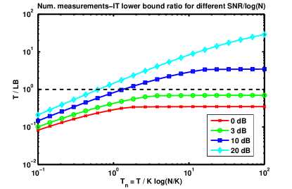
Next, we compare with the bounds for exact recovery derived in [20] where we have , and . For this setup, we prove that is a necessary condition for recovery and for that SNR, is necessary for sublinear , and sufficient in the same regime for recovery with a vanishing fraction of support errors, which matches the conditions derived in [20] for the corresponding sparsity conditions.
We remark that regime in this model roughly corresponds to the regime in [19, 22]. We also note that while having depend on complicates the derivation of lower and upper bounds, this scaling ensures normalized columns and conveniently decouples the effects of SNR and the number of measurements. The decoupling leads to the aforementioned lower bound on SNR that is independent of the number of measurements.
We now provide the analysis to obtain the above conditions given Theorem VI.1. We first show that is necessary for recovery. For any , or SNR assume scales much faster, e.g. , such that
since for . Then, the necessary condition given by (30) is
which readily leads to the condition that
| (33) |
for constant . Note that, if the condition above is necessary for any , it is also necessary for smaller scalings of .
For the lower bound, we consider sublinear sparsity and and prove that is necessary by contradiction. Let and assume that , where . In the left-hand side of the inequality (30), we have , while on the right-hand side we have
for some constant noting that . Canceling the terms on each side we have and therefore the inequality is not satisfied for any .
We now show that is a sufficient condition for and . For , the right-hand side in the sufficient condition given in (32) is
where we note that for all in this scaling regime. For above is equivalent to . For we have the denominator therefore the term above is again . Thus satisfies (32).
In Figure 2, we illustrate the lower bound on the number of observations for the setup of [20], which shows that a necessary condition on SNR has to be satisfied for recovery, as we have stated above.
Remark VI.1.
We showed that our relatively simple mutual information analysis gives us upper and lower bounds that are asymptotically identical to the best-known bounds obtained through problem-specific analyses in [19, 22, 20] in their respective setups for most scaling regimes of interest.
We also note that while the aforementioned work analyze bounds assuming a lower bound on the power of the support coefficients , our lower bound analysis proves that such a lower bound is required for recovery. For instance, assuming there exists any one index such that with non-zero probability, for we would obtain , showing that recovery is impossible due to Theorem IV.1.
Another interesting aspect of our analysis is that in addition to sample complexity bounds, an upper bound to the probability of error in recovery can be explicitly computed and obtained using Lemma V.2 for any finite triplet , using the error exponent obtained in Section -F. Following this line of analysis, an upper bound is obtained for sparse linear regression and compared to the empirical performance of practical algorithms such as Lasso [15, 13] in [2]. It is then seen that while certain practical recovery algorithms have provably optimal asymptotic sample complexity, there is still a gap between information-theoretically attainable recovery performance and the empirical performance of such algorithms. We refer the reader to [2] for details.
VI-B Regression with Correlated Support Elements
In the following subsections we consider several variants of the sparse linear regression problem with different setups. First, we consider a variant where the support elements are correlated, in contrast to the IID assumption we had in the previous section. Note that we are still considering recovery in a Bayesian setting for rather than a worst-case analysis. Having correlated elements in the support usually complicates the analysis when using problem-specific approaches, however, in our framework the analysis is no different than the IID case. We even obtain slightly improved bounds (which we detail shortly) as a result of correlation decreasing the uncertainty in the observation model.
Formally, we consider the same problem setup as above, except that is not IID and we assume . A special case of such a correlated setup is when the distribution has finite volume on its support, for which we have . We note that the correlation in does not affect the mutual information computation for nor the analysis to show that the regularity conditions (RC1-2) hold. The only change in the analysis is that the Rényi entropy term in the numerator of Theorem V.2 is now asymptotically dominated by the combinatorial term for all . Thus, we can improve the upper bound for scaling in (32) from recovery with a vanishing fraction of errors to exact recovery, and from to to obtain the following theorem as the analogue of Theorem VI.1.
Theorem VI.2.
For sparse linear regression with correlated support elements , a necessary condition on the number of measurements for exact recovery of the support is
| (34) |
and a sufficient condition for exact recovery is
| (35) |
for a constant .
VI-C Sensing Matrices with Correlated Columns
We consider another extension to the typical sparse linear regression setup in Section VI-A, where we have correlated columns in the sensing matrix . As with correlated support coefficients, this is yet another setup whose analysis in the classical sparse linear regression literature is inherently more cumbersome than the IID case. While our problem setup does not support non-IID variables , we consider a simple extension that appeared in previous work in [2] and show that correlation only affects the effective SNR, and up to a constant amount of correlation can be theoretically tolerated. This result is in contrast to the earlier results concerning the performance of algorithms such as Lasso, which considered decaying correlations [15]. An information-theoretic analysis of this setup has also been considered in [18].
Formally, we consider the setup of Section VI-A, with the difference that for any two elements in , , on a row of , we have a correlation coefficient . For instance for the setup of [20], this corresponds to . We remark that this probabilistic model is equivalent to the following one: Let , where and where is IID across . As a result, we have that for are conditionally IID given the latent factor .
We note that the general framework we consider in Sections IV and V explicitly necessitates IID variables . However, this setup can be naturally extended to conditionally IID variables conditioned on a latent factor (see [2] for details). It turns out that most of the results from Sections IV and V readily generalize to this model, with the dependence having the effect that the mutual information expressions are additionally conditioned on the latent factor , i.e., .
With the extension to conditionally IID variables considered in [2] and the formulation of the correlated columns setup as conditionally IID columns given , the mutual information expressions and regularity conditions conditioned on can be explicitly computed. With these results, we observe that the correlated columns problem is equivalent to the IID problem except that the “effective SNR” , where SNR denotes the signal to noise ratio for the IID problem. This leads to the conclusion that up to a constant correlation can be tolerated for recovery, in contrast to older results on the analysis of recovery algorithms such as Lasso which required decaying correlations, e.g. [15]. We refer the reader to [2] for extension to the conditionally IID framework, along with analysis and numerical experiments for the correlated sensing columns setup.
VI-D Bouquet Model for Support Elements
In this subsection, we consider another variation of the linear regression problem, where for each sample ,
with each having the same support , but different coefficients obeying a “bouquet model”
We assume is IID across samples and is described by a zero-mean Gaussian with variance . The aforementioned model is an example of linear regression models with “time-varying” support, which have been previously considered in the literature [40].
In order to analyze this model in our general framework, we remark that can be considered a latent observation model parameter that is constant across , corresponding to in our setup in Section III. The “noise” in , , can simply be incorporated into the observation model . A straightforward analysis of the mutual information using Jensen’s inequality arguments similar to the proof of Theorem VII.2 (omitted here for brevity) reveals that a lower bound on is . Thus, we can obtain an upper bound on the number of measurements similar to (31), where we show the effect of noise in to be equivalent to measurement noise with variance as opposed to .
Remark VI.2.
We remark that the mutual information analysis can be easily performed for different distributions (other than Gaussian) on the sensing matrix elements and the measurement noise . It is only necessary to compute the mutual information for the different probability distributions and ensure that the smoothness conditions (RC1-2) hold, if an upper bound for scaling models is desired. This is another advantage to our unifying framework, since problem-specific approaches need significantly different analyses to extend to different distributions of sensing matrices and measurement noise.
VI-E Multivariate Regression
In this problem, we consider the following linear model [7], where we have a total of linear regression problems,
For each , is a -sparse vector, and . The relation between different tasks is that have joint support . This setup is also called multiple linear regression or distributed compressive sensing [8] and is useful in applications such as multi-task learning [41].
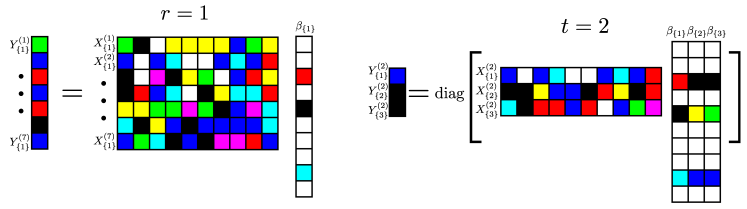
It is easy to see that this problem can be formulated in our sparse recovery framework, with vector-valued outcomes and variables . Namely, let be a vector-valued outcome, be the collection of vector-valued variables and be the collection of sparse vectors sharing support , making it block-sparse. This mapping is illustrated in Figure 3. Assuming independence between and support coefficients across , we have the following observation model:
We state the following theorem for the specific linear model in Section VI-A, as a direct result of Theorem VI.1 and the fact that the joint mutual information decomposes to identical mutual information terms in view of the equality above.
Theorem VI.3.
Remark VI.3.
We showed that having problems with independent measurements and sparse vector coefficients decreases the number of measurements per problem by a factor of . While having such problems increases the number of measurements -fold, the inherent uncertainty in the problem is the same since the support is shared. It is then reasonable to expect such a decrease in the number of measurements.
VII Applications with Nonlinear Observations
In this section, we consider several problems where the relationship between the input variables and the observations are nonlinear. We first look at a general framework where some of the variables are not observed, i.e., each variable is missing with some probability. We then analyze probit regression and group testing problems as other examples of problems with nonlinear observations.
VII-A Models with Missing Features
Consider the general sparse signal processing model as described in Section III. However, assume that instead of fully observing outcomes and features , we observe a matrix instead of , with the relation
i.e., we observe a version of the feature matrix which may have entries missing with probability , independently for each entry. We show how the sample complexity changes relative to the case where the features are fully observed. The missing data setup for specific problems have previously been considered in the literature [6, 32].
First we present a universal lower bound on the number of samples for the missing data framework, by relating to .
Theorem VII.1.
Consider the missing data setup described above. Then we have the lower bound on the sample complexity , where is the lower bound on the sample complexity for the fully observed variables case given in Theorem IV.1.
Proof.
We compute in terms of . To do that, we compute for any set . To simplify the expressions, we omit the conditioning on and in all entropy and mutual information expressions below.
| (36) | ||||
| (37) | ||||
| (38) | ||||
| (39) | ||||
| (40) | ||||
| (41) | ||||
| (42) |
(36), (37) and (38) follow from the chain rule of entropy. (39) follows from the conditional independence of and given and the independence of over . In (40), we explicitly write the conditional entropies for two values of . These expressions simplify to (41) and we group the terms over to obtain (42).
For any set with elements , we can write
| (43) | ||||
| (44) | ||||
| (45) | ||||
| (46) |
where (43) follows from the chain rule and the independence of and given , (44) by expanding the conditioning on , (45) from the definition of mutual information and (46) from the chain rule.
W.l.o.g., assume and . Finally, using the above expressions we have
The first two equalities follow from the expressions we found earlier and the third equality follows from the definition of the mutual information by rearranging the sums and using the chain rule of mutual information. The last inequality follows from the non-negativity of mutual information and expanding the mutual information expressions in the first set of parentheses. The lower bound then follows from Theorem IV.1. ∎
As a special case, we analyze the sparse linear regression model with missing data [6, 32], where we obtain a model-specific upper bound on the sample complexity, in addition to the universal lower bound given by Theorem VII.1. We consider the setup of [19, 22] in the lower SNR regime , however analogous results can be shown for higher SNR regimes or for the setup of [20]. The proof is given in the appendix.
Theorem VII.2.
Remark VII.1.
We observe that the number of sufficient samples increases by a factor of for missing probability . Compare this to the upper bound given by [32] with scaling , where the authors propose and analyze an orthogonal matching pursuit algorithm to recover the support with noisy or missing data. In this example, we have shown an upper bound that improves upon the bounds in the literature, with an intuitive universal lower bound.
This example highlights the flexibility of our results in view of the mutual information characterization. This flexibility enables us to easily compute new bounds and establish new results for a very wide range of general models and their variants.
VII-B Binary Regression
As an example of a nonlinear observation model, we look at the following binary regression problem, also called 1-bit compressive sensing [11, 25, 42] or probit regression. Regression with 1-bit measurements is interesting as the extreme case of regression models with quantized measurements, which are of practical importance in many real world applications. The conditions on the number of measurements have been studied for both noiseless [25] and noisy [42] models and has been established as a sufficient condition for Gaussian variable matrices.
Following the problem setup of [42], we have
| (47) |
where is a matrix with IID standard Gaussian elements, and is an vector that is -sparse with support . We assume for for a constant . is a noise vector with IID standard Gaussian elements. is a 1-bit quantizer that outputs if the input is non-negative and otherwise, for each element in the input vector. This setup corresponds to the constant SNR regime in [42]. We consider the constant regime and use the results of Theorem V.1 to write the following theorem.
Theorem VII.3.
For probit regression with IID Gaussian variable matrix and the above setup, measurements are sufficient to recover , the support of , with an arbitrarily small average error probability.
The proof is provided in the appendix.
Remark VII.2.
Similar to linear regression, for probit regression with noise we provided a sufficiency bound that matches [42] for an IID Gaussian matrix, for the corresponding SNR regime.
We note that a lower bound on the number of measurements can also be obtained trivially, since the mutual information is upper bounded by the entropy of the measurement . Since we consider binary measurements, this leads to the lower bound for exact recovery through Theorem IV.1.
VII-C Group Testing - Boolean Model
In this section, we consider another nonlinear model, namely, group testing. This problem has been covered comprehensively in [5] and the results derived therein can also be recovered using the generalized results we presented in this paper as we show below.
The problem of group testing can be summarized as follows. Among a population of items, unknown items are of interest. The collection of these items represents the defective set. The goal is to construct a pooling design, i.e., a collection of tests, to recover the defective set while reducing the number of required tests. In this case is a binary measurement matrix defining the assignment of items to tests. For the noise-free case, the outcome of the tests is deterministic. It is the Boolean sum of the codewords corresponding to the defective set , given by .
Note that for this problem there does not exist a latent observation parameter . Therefore we have as the mutual information quantity characterizing the sample complexity for zero error recovery.
Theorem VII.4.
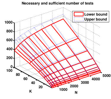
For items and defectives, the number of tests is necessary for and sufficient for , to identify the defective set exactly with an arbitrarily small average error probability.
We prove the theorem in the appendix. The upper and lower bounds on the number of tests (given by Theorem V.2 and IV.1 respectively) for the noiseless case are illustrated in Figure 4. The results in [5] also establish upper and lower bounds on the number of tests needed for testing with additive noise (leading to false alarms) and dilution effects (leading to potential misses), as well as worst-case errors.
We remark that we have been able to remove the extra polylog factor in in the upper bound of [5] and extended the regime of the upper bound from to with the result above.
VIII Conclusions
We have presented a unifying framework based on noisy channel coding for analyzing sparse recovery problems. This approach unifies linear and nonlinear observation models and leads to explicit, intuitive and universal mutual information formulas for computing the sample complexity of sparse recovery problems. We explicitly focus on the inference of the combinatorial component corresponding to the support set, provably the main difficulty in sparse recovery. We unify sparse problems from an inference perspective based on a Markov conditional independence assumption. Our approach is not algorithmic and therefore must be used in conjunction with tractable algorithms. It is useful for identifying gaps between existing algorithms and the fundamental information limits of different sparse models. It also provides an understanding of the fundamental tradeoffs between different parameters of interest such as , , SNR and other model parameters. It also allows us to obtain new or improved bounds for various sparsity-based models.
-A First Derivative of and Mutual Information
Below, we use notation for discrete variables and observations, i.e. sums, however the expressions are valid for continuous models if the sums are replaced by the appropriate integrals arising in the mutual information definition for continuous variables. Let , where we omit the dependence of on , and . Then note that . For the derivative w.r.t. we then have
Henceforth, we only consider the numerator since the denominator is obviously equal to 1 at . For the derivative of we have
therefore . For the second term, we have and using the independence of and in the last equality, we can rewrite the numerator as
| (A.1) |
-B Proof of Lemma V.2 and Extension to Continuous Models
Proof of Lemma V.2
As we note in the main section, the proof of the lemma follows along the proof of Lemma III.1 in [5] which considers binary alphabets in [5], yet readily generalizes to discrete alphabets for and . However, because of the latent variables , the final step in the bottom of p. 1888 of [5] does not hold true and the proof ends with the previous equation. As a result, we have the upper bound
| (A.2) |
for the multi-letter error exponent defined as
| (A.3) |
Note that we obtain the conditioning on since we consider the ML decoder conditioned on that event and we write .
Furthermore, note that Lemma V.2 is missing a multiplying the term compared to Lemma III.1 in [5]; this is due to the fact that we do not utilize the stronger proof argument in Appendix A of [5], but rather follow from the argument provided in the proof in the main body, as in [43]. Using that argument, Lemma V.2 can be obtained by modifying inequality (c) in p. 1887 that upper bounds such that is replaced with .
To obtain Lemma V.2, we relate this multi-letter error exponent to the single-letter error exponent which we defined in (21). The following lower bound removes the dependence between samples by considering worst-case and reduces it to a single-letter expression.
Lemma .1.
Continuous models
Even though the results and proof ideas that were used in Sections V and IV are fairly general, the proof of Lemma V.2 holds for discrete variables and outcomes using the proof above. In this section, we make the necessary generalizations to state an analogue of Lemma V.2 for continuous variable and observation models, specifically for the case . The extension to finite dimensional real coordinate spaces follows through the same analysis as well. We follow the methodology in [36] and [44].
To simplify the exposition, we consider the extension to continuous variables in the special case of fixed and known . In that case, as defined in (21) reduces to
| (A.4) |
for with .
We assume a continuous and bounded joint probability density function with joint cumulative distribution function . The conditional probability density for the observation model is assumed to be a continuous and bounded function of both and .
Let be the random vector and be the random variable generated by the quantization of and , respectively, where each variable in is quantized to values and quantized to values. Let be the joint cumulative distribution function of . As before, let be the ML decoder with continuous inputs with probability of making errors in decoding denoted by . Let be the ML decoder that quantizes inputs and to and , and have the corresponding probability of error . Define
where the indexing denotes the random variates that the error exponents are computed with respect to.
Utilizing Lemma V.2 for discrete models, we will show that an analogue of the lemma holds for the continuous model, i.e.,
| (A.5) |
The rest of the proof of Theorem V.1 will then follow as in the discrete case, by noting that , with the mutual information definition for continuous variables [3].
Our approach can be described as follows. We will increase the number of quantization levels for and , respectively. Then, since the discrete result in (20) holds for any number of quantization levels, by taking limits we will be able to show that
| (A.6) |
Since is the minimum probability of error decoder, any upper bound for will also be an upper bound for , thereby proving (A.5).
Assume is quantized with the quantization boundaries denoted by , with if . For convenience denote and . Furthermore, assume the quantization boundaries are equally spaced, i.e. for . Now, we have that
| (A.7) | |||||
| (A.8) | |||||
| (A.9) | |||||
| (A.10) | |||||
Let and for each choose the sequence of quantization boundaries such that , , . Then, the last two terms disappear and using the fundamental theorem of calculus, we obtain
| (A.11) |
It can also be shown that increases for finer quantizations of , therefore gives the smallest upper bound over over the quantizations of , similar to [36]. However, this is not necessary for the proof.
We repeat the same procedure for . Assume each variable in is quantized with the quantization boundaries denoted by , with if . For convenience denote and . Furthermore, assume that the quantization boundaries are equally spaced, i.e. for . Then, we can write
| (A.12) | |||||
| (A.13) | |||||
| (A.14) | |||||
where (A.13) follows with being the step function that represents the cumulative distribution function of the quantized variables .
Let , for each choose a set of quantization points such that , , . Again, the second and third terms disappear and the first sum converges to the integral over . Note that is a bounded continuous function of all its variables since it was assumed that and were bounded and continuous. Also note that , which implies the weak convergence of the probability measure of to the probability measure of . Given these facts, using the portmanteau theorem we obtain that , which leads to
| (A.15) |
This leads to the following result, completing the proof.
| (A.16) |
-C Proof of Lemma .1
As in the previous proofs, while we use notation for discrete variables and observations, the proof below is valid for continuous models. We omit the conditioning on and let denote the probability distribution and the Rényi entropy of conditioned on w.l.o.g.
For the error exponent as defined in (A.3), let
such that . We then write the following chain of inequalities:
where the first inequality follows from the subadditivity of exponentiating with and the second follows by multiplying and dividing inside the sum by and defining . The third inequality follows using Jensen’s inequality. We obtain the final expression by noting that the expression in the square brackets factorizes over and is IID over when conditioned on .
Noting that , where is the Rényi entropy of order , we then have
-D Proof of Lemma V.3
Let be a countable dense subset and w.l.o.g. write . We also note that since is monotone in and its limit is continuous w.r.t. , it follows that is equicontinuous in .
Let . Then, for all , there exists such that for all uniformly due to the aforementioned equicontinuity. depends on but not on due to equicontinuity.
Let . Then, for all , there exists such that for all such that due to the continuity of w.r.t. . depends on and , which in turn depends only on .
Let . Then, for all , there exists such that for all , for all uniformly due to the uniform convergence of to w.r.t. . depends on , which in turn depends only on . This implies that for ,
which follows from the triangle inequality.
Define the collection of sets , where is the open ball with radius and center . Note that is an open cover of since for all and we chose to be a dense subset of . Since is compact, it then follows that there exists a finite subcover of . W.l.o.g. let for a constant integer . Also, define the constants and , for which we have and .
Let . Since is a finite cover of , there exists such that . This implies that for all ,
where in the first inequality we used the fact that is non-decreasing in and . Choosing such that proves the lemma.
The necessity of compactness and uniform convergence assumptions are apparent from the proof. Without compactness, we cannot find a finite subcover and if we selected and , we are not guaranteed that and . Similarly, without uniform convergence the sequence index for which for would depend on and we cannot find a to upper bound over all .
-E Proof of Theorem V.3
We first distingiush between two scaling regimes, namely and . For the first regime, we remark that is always asymptotically dominated by , thus the condition (27) in Theorem V.2 reduces to (28) in Theorem V.3. This implies that we are able to obtain exact recovery, i.e. in the setup considered in Theorem V.3 if . Thus in the rest of the proof we deal with the case .
Consider a sequence of numbers , representing the fraction of errors in the support that we would like to allow for each . Define the corresponding sequence of error events , where each is the event that the recovered set has more than errors, i.e., . We assume for notational convenience that correspond to integers.
From the end of proof of Theorem V.2, we have that for satisfying condition (27),
for constants . Since we have , it then follows that
Let . For this and , we have
since . Thus for this choice of we again have that is asymptotically dominated by . This implies that the above bound on can be achieved with the condition (28) on rather than (27).
Investigating the upper bound on the error probability for this choice of , we have
for some constant . To see that the last equivalence holds, take the of both sides, where for the left-hand side we have . If we show that this term is lower bounded by for any constant it implies that the equivalence holds. Using the fact that , we can first lower bound this term by for any (arbitrarily large) constant . Then, since we can again lower bound the term by , proving the equivalence.
With this scaling on , we then have that and it follows from the Borel-Cantelli lemma that . Writing the explicitly, we have
thus with probability one and the theorem follows.
-F Sparse Linear Regression Analysis
Error exponent and regularity conditions
We now compute the error exponent similar to [2], where and where . While we can obtain an upper bound directly using Lemma V.2 and the computed error exponent, we use this computation to show that the regularity conditions (RC1-2) hold for Theorem V.2.
We can write
and below we compute the inner expectation over .
where , , , and . Then taking the integral, some terms on the left cancel and we have
| (A.17) |
Writing the second integral that is over , we then have
where , and . Again, evaluating the integral, we obtain
Integrating the above expression w.r.t. , we see that
By the matrix determinant lemma, we have and by the Sherman-Morrison formula, . Similarly, and . By plugging in these expressions, we can then see that and . We simplify the above expression to obtain
| (A.18) |
and therefore letting and , we have
| (A.19) |
From above, it is now obvious that (RC1) is satisfied since , which is a finite interval independent of . It also follows from straightforward algebra that
We assume is monotonic with and consider three cases for the limit : , or . In the first case we have and in the second case . In all three cases it is obvious that is continuous in for all . To prove uniform convergence in , we claim that is a monotonically non-decreasing or non-increasing sequence for each and . For the first case, for large enough we observe that , which is monotone in . For the second case, for large enough , which is also monotone in . For the third case is constant w.r.t. and thus also monotone. Then by Dini’s Theorem we have that converges uniformly in , proving that (RC2) holds.
-G Proof of Theorem VII.2
Let and for , define and . For simplicity of exposition, we will assume the worst-case support with any such that for , however the results can be generalized to random similar to the proof of Theorem VI.1. We also omit the explicit conditioning on and in the expressions below.
To prove the theorem, we will obtain a lower bound on . Let and denote the set of missing features in each set, then it simply follows that and .
We will start by proving an upper bound on . We have,
The first two equalities follow by expanding and , . The third equality follows by subtracting the known quantities related to from the entropy expression. The fourth equality follows by noting that the variable inside the entropy conditioned on and is Gaussian and then computing its variance. We use Jensen’s inequality over by noting that is a concave function to obtain the inequality. We then note that is a binomially distributed random variable with expectation .
Similar to what we did for , we can also write
Combining the two entropy expressions, we then have
Note that the expression above reduces to the expression for the fully observed case for .
Now consider the low SNR setup of [19, 22], where , . Then, for the mutual information we have,
where the last equivalence can be shown by considering the two regimes and separately. It then follows that is sufficient for exact recovery for correlated and or sufficient for recovery with a vanishing fraction of support errors for IID and , similar to the results in Section VI-A and VI-B.
-H Proof of Theorem VII.3
In order to obtain the model-specific bounds, for a subset we analyze the mutual information term which is lower bounded by for any realization of . Therefore, w.l.o.g. we consider for and omit the conditioning on and for brevity.
We write the mutual information term as
where we will analyze and to obtain a lower bound for the mutual information expression.
Defining , and , we have since the quantizer input depends only on the sum of the elements of . Note that with , with . Now we explicitly write the conditional entropy
| (A.20) |
with and , which can be written as
where and the function defined as .
Then, we write the following chain of inequalities:
| (A.23) | ||||
| (A.24) | ||||
| (A.25) | ||||
| (A.26) | ||||
| (A.27) |
Equality (A.23) follows from the evenness of the function inside the integral and we write (A.24) by noting that and are non-negative. is expanded and the bounds above for the function are used to obtain (A.25) and (A.26) is a regrouping of terms by defining and rewriting the limits of the integral by noting that the integrand is an even function. We obtain (A.27) by evaluating the integral. For , we have
where we define and replacing , and , we can then write
| (A.28) | ||||
| (A.29) |
We now analyze the second term to obtain an upper bound. Again, note that , then
where this time we define and , which can be written as
Then, write the following chain of inequalities:
| (A.30) | ||||
| (A.31) | ||||
| (A.32) | ||||
| (A.33) | ||||
| (A.34) |
Equality (A.30) follows from the evenness of the function inside the integral and we write (A.31) by noting that for . is expanded and the above bounds for the function are used to obtain (A.32) and (A.33) is a regrouping of terms by defining and rewriting the limits of the integral by noting that the integrand is an even function. We obtain (A.27) by evaluating the integral. Replacing , we then have
| (A.35) |
-I Proof of Theorem VII.4
We start by considering the error exponent for for and define (not necessarily constant). We remark that does not exist for this problem, thus we can ignore the Rényi entropy term and the minimization over .
Notice that the observation model depends only on and and and are Bernoulli random variables with parameters and , respectively. Thus, we can rewrite the expression above as
where if and 0 otherwise. Since this is a binary function, it is not affected by the exponentiation with and we can further simplify the expression above as
For the realization , the inner sum turns out to be , while for the realization we obtain . We can then write the error exponent to be exactly . Notice that for large enough , behaves as , while behaves as .
With this asymptotic consideration, and by letting , we obtain . With some algebra, we see that this is equal to , thus we have , for both and .
Now we can simply show that for . For , it follows that for a large enough constant , thus proving the upper bound for . The lower bound can be obtained by noting that as for the binary regression case.
References
- [1] C. Aksoylar, G. Atia, and V. Saligrama, “Sample complexity of salient feature identification for sparse signal processing,” in Proc. IEEE Statistical Signal Processing Workshop (SSP), Aug. 2012, pp. 329–332.
- [2] C. Aksoylar and V. Saligrama, “Information-theoretic characterization of sparse recovery,” in Proc. of the Seventeenth Int. Conf. on Artificial Intelligence and Statistics (AISTATS), Reykjavik, Iceland, April 2014, pp. 38–46.
- [3] T. M. Cover and J. A. Thomas, Elements of Information Theory. New York: John Wiley and Sons, Inc., 1991.
- [4] D. L. Donoho, “Compressed sensing,” IEEE Trans. Inf. Theory, vol. 52, no. 4, pp. 1289–1306, April 2006.
- [5] G. Atia and V. Saligrama, “Boolean compressed sensing and noisy group testing,” IEEE Trans. Inf. Theory, vol. 58, no. 3, March 2012.
- [6] P.-L. Loh and M. Wainwright, “High-dimensional regression with noisy and missing data: Provable guarantees with non-convexity,” in Advances in Neural Information Processing Systems (NIPS), 2011, pp. 2726–2734.
- [7] S. Negahban and M. Wainwright, “Joint support recovery under high-dimensional scaling: Benefits and perils of -regularization,” in Advances in Neural Information Processing Systems (NIPS), 2008.
- [8] M. B. Wakin, S. Sarvotham, M. F. Duarte, D. Baron, and R. G. Baraniuk, “Recovery of jointly sparse signals from few random projections,” in Proc. of the Workshop on Neural Information Processing Systems (NIPS), Vancouver, Canada, Dec. 2005, pp. 1435–1442.
- [9] J. Qian and V. Saligrama, “Efficient minimax signal detection on graphs,” in Advances in Neural Information Processing Systems (NIPS), Z. Ghahramani, M. Welling, C. Cortes, N. D. Lawrence, and K. Q. Weinberger, Eds. Curran Associates, Inc., 2014, pp. 2708–2716.
- [10] J. Qian, V. Saligrama, and Y. Chen, “Connected sub-graph detection,” in Proc. of the Seventeenth Int. Conf. on Artificial Intelligence and Statistics (AISTATS), Reykjavik, Iceland, April 2014, pp. 796–804.
- [11] P. T. Boufounos and R. G. Baraniuk, “1-bit compressive sensing,” in Proc. of Conf. on Information Sciences and Systems (CISS), March 2008, pp. 16–21.
- [12] Y. Plan and R. Vershynin, “Robust 1-bit compressed sensing and sparse logistic regression: A convex programming approach,” IEEE Trans. Inf. Theory, vol. 59, no. 1, pp. 482–494, Jan 2013.
- [13] M. J. Wainwright, “Sharp thresholds for high-dimensional and noisy sparsity recovery using -constrained quadratic programming (lasso),” IEEE Trans. Inf. Theory, vol. 55, no. 5, pp. 2183–2202, May 2009.
- [14] A. K. Fletcher, S. Rangan, and V. K. Goyal, “Necessary and sufficient conditions for sparsity pattern recovery,” IEEE Trans. Inf. Theory, vol. 55, no. 12, pp. 5758–5772, 2009.
- [15] E. J. Candès and Y. Plan, “Near-ideal model selection by minimization,” Ann. Statist., vol. 37, no. 5A, pp. 2145–2177, 2009.
- [16] V. Saligrama and M. Zhao, “Thresholded basis pursuit: LP algorithm for order-wise optimal support recovery for sparse and approximately sparse signals from noisy random measurements,” IEEE Trans. Inf. Theory, vol. 57, no. 3, pp. 1567–1586, 2011.
- [17] M. Akcakaya and V. Tarokh, “Shannon-theoretic limits on noisy compressive sampling,” IEEE Trans. Inf. Theory, vol. 56, no. 1, pp. 492–504, Jan. 2010.
- [18] M. J. Wainwright, “Information-theoretic limits on sparsity recovery in the high-dimensional and noisy setting,” IEEE Trans. Inf. Theory, vol. 55, no. 12, pp. 5728–5741, 2009.
- [19] W. Wang, M. J. Wainwright, and K. Ramchandran, “Information-theoretic limits on sparse signal recovery: Dense versus sparse measurement matrices,” IEEE Trans. Inf. Theory, vol. 56, no. 6, pp. 2967–2979, June 2010.
- [20] S. Aeron, M. Zhao, and V. Saligrama, “Information theoretic bounds for compressed sensing,” IEEE Trans. Inf. Theory, vol. 56, no. 10, pp. 5111–5130, Oct. 2010.
- [21] G. Reeves and M. C. Gastpar, “Approximate sparsity pattern recovery: Information-theoretic lower bounds,” IEEE Trans. Inf. Theory, vol. 59, no. 6, pp. 3451–3465, June 2013.
- [22] K. Rahnama Rad, “Nearly sharp sufficient conditions on exact sparsity pattern recovery,” IEEE Trans. Inf. Theory, vol. 57, no. 7, pp. 4672–4679, July 2011.
- [23] Y. Jin, Y.-H. Kim, and B. D. Rao, “Limits on support recovery of sparse signals via multiple-access communication techniques,” IEEE Trans. Inf. Theory, vol. 57, no. 12, pp. 7877–7892, Dec 2011.
- [24] G. Tang and A. Nehorai, “Performance analysis for sparse support recovery,” IEEE Trans. Inf. Theory, vol. 56, no. 3, pp. 1383–1399, 2010.
- [25] L. Jacques, J. N. Laska, P. T. Boufounos, and R. G. Baraniuk, “Robust 1-bit compressive sensing via binary stable embeddings of sparse vectors,” IEEE Trans. Inf. Theory, vol. 59, no. 4, pp. 2082–2102, April 2013.
- [26] C. L. Chan, S. Jaggi, V. Saligrama, and S. Agnihotri, “Non-adaptive group testing: Explicit bounds and novel algorithms,” in Proc. of the Int. Symp. on Information Theory (ISIT), July 2012, pp. 1837–1841.
- [27] M. B. Malyutov and P. S. Mateev, “Planning of screening experiments for a nonsymmetric response function,” Mat. Zametki, vol. 27, no. 1, pp. 109–127, 1980.
- [28] M. B. Malyutov, “On planning of screening experiments,” in Proceedings of 1975 IEEE-USSR Workshop on Inf. Theory, 1976.
- [29] ——, “The separating property of random matrices,” Mat. Zametki, vol. 23, no. 1, pp. 155–167, 1978.
- [30] ——, “Maximal rates of screening designs,” Probab. Appl., vol. 24, 1979.
- [31] A. Dyachkov, “Lectures on designing screening experiments,” Moscow State Univ., 2003.
- [32] Y. Chen and C. Caramanis, “Noisy and missing data regression: Distribution-oblivious support recovery,” in International Conference on Machine Learning, 2013.
- [33] C. Aksoylar, G. Atia, and V. Saligrama, “Compressive sensing bounds through a unifying framework for sparse models,” in Proc. of the IEEE Int. Conf. on Acoustics, Speech, and Signal Processing (ICASSP), May 2013.
- [34] ——, “Sparse signal processing with linear and non-linear observations: A unified Shannon theoretic approach,” in Proc. of the IEEE Inf. Theory Workshop (ITW), Seville, Spain, 2013.
- [35] C. Aksoylar and V. Saligrama, “Information-theoretic bounds for adaptive sparse recovery,” in Proc. of the Int. Symp. on Information Theory (ISIT), 2014, pp. 1311–1315.
- [36] R. G. Gallager, Information Theory and Reliable Communication. New York, NY, USA: John Wiley & Sons, Inc., 1968.
- [37] G. Atia and V. Saligrama, “Boolean compressed sensing and noisy group testing,” arXiv pre-print, arXiv:0907.1061v2, Nov 2009.
- [38] A. El Gamal and Y.-H. Kim, “Elements of network information theory,” 2012.
- [39] X. Chen and D. Guo, “Gaussian many-access channels: Definition and symmetric capacity,” in IEEE Information Theory Workshop (ITW), Seville, Spain, 2013.
- [40] N. Vaswani, “Kalman filtered compressed sensing,” in Proc. of the 15th IEEE Int. Conf. on Image Processing (ICIP), 2008, pp. 893–896.
- [41] A. Jalali, P. Ravikumar, S. Sanghavi, and C. Ruan, “A dirty model for multi-task learning,” in Advances in Neural Information Processing Systems (NIPS), 2010, pp. 964–972.
- [42] A. Gupta, R. Nowak, and B. Recht, “Sample complexity for 1-bit compressed sensing and sparse classification,” in Proc. of the Int. Symp. on Information Theory (ISIT), June 2010, pp. 1553–1557.
- [43] G. K. Atia, V. Saligrama, and C. Aksoylar, “Correction to “Boolean compressed sensing and noisy group testing”,” IEEE Trans. Inf. Theory, vol. 61, no. 3, pp. 1507–1507, 2015.
- [44] R. G. Gallager, “Information theory,” in Mathematics of Physics and Chemistry, Vol. 2. Princeton, NJ, USA: Van Nostrand, 1964.
- [45] M. Chiani, D. Dardari, and M. K. Simon, “New exponential bounds and approximations for the computation of error probability in fading channels,” IEEE Trans. Wireless Commun., vol. 2, no. 4, pp. 840–845, July 2003.
- [46] G. T. F. de Abreu, “Supertight algebraic bounds on the Gaussian Q-function,” in Asilomar Conference on Signals, Systems and Computers, Nov. 2009, pp. 948–951.
| Cem Aksoylar received the B.Sc. degree in electronics engineering from Sabanci University, Istanbul, Turkey in 2010. He is currently working towards the Ph.D. degree in electrical and computer engineering in Boston University, MA. His research interests include statistical signal processing, high dimensional learning problems and inference and optimization over networks. |
| George K. Atia (S’01–M’09) received the B.Sc. and M.Sc. degrees from Alexandria University, Egypt, in 2000 and 2003, respectively, and the Ph.D. degree from Boston University, MA, in 2009, all in electrical and computer engineering. He joined the University of Central Florida in Fall 2012, where he is currently an assistant professor and a Charles N. Millican Faculty Fellow in the Department of Electrical and Computer Engineering. From Fall 2009 to 2012, he was a postdoctoral research associate at the Coordinated Science Laboratory (CSL) at the University of Illinois at Urbana-Champaign (UIUC). His research interests include statistical signal processing, machine learning, stochastic control, wireless communications, detection and estimation theory, and information theory. Dr. Atia is the recipient of many awards, including the NSF CAREER Award in 2016, the Outstanding Graduate Teaching Fellow of the Year Award in 2003–2004 from the Electrical and Computer Engineering Department at Boston University, the 2006 College of Engineering Dean’s Award at the BU Science and Engineering Research Symposium, and the best paper award at the International Conference on Distributed Computing in Sensor Systems (DCOSS) in 2008. |
| Venkatesh Saligrama is a faculty member in the Department of Electrical and Computer Engineering and Department of Computer Science (by courtesy) at Boston University. He holds a Ph.D. from MIT. His research interests are in statistical signal processing, machine learning and computer vision, information and decision theory. He has edited a book on Networked Sensing, Information and Control. He has served as an Associate Editor for IEEE Transactions on Information Theory, IEEE Transactions on Signal Processing and has been on Technical Program Committees of several IEEE conferences. He is the recipient of numerous awards including the Presidential Early Career Award (PECASE), ONR Young Investigator Award, and the NSF Career Award. More information about his work is available at http://sites.bu.edu/data. |