Two-time free energy distribution function in (1+1) directed polymers

Abstract

Two time free energy distribution function in one-dimensional directed polymers in random potential is derived in terms of the Bethe ansatz replica technique by mapping the replicated problem to the $N$-particle quantum boson system with attractive interactions.

I Introduction

We consider the model of directed polymers defined in terms of an elastic string $\phi(\tau)$ directed along the $\tau$-axes within an interval $[0,t]$ which passes through a random medium described by a random potential $V(\phi,\tau)$. The energy of a given polymer’s trajectory $\phi(\tau)$ is

$$H[\phi(\tau),V]=\int_{0}^{t}d\tau\Bigl{\{}\frac{1}{2}\bigl{[}\partial_{\tau}\phi(\tau)\bigr{]}^{2}+V[\phi(\tau),\tau]\Bigr{\}};$$ (1)

where the disorder potential $V[\phi,\tau]$ is Gaussian distributed with a zero mean $\overline{V(\phi,\tau)}=0$ and the $\delta$-correlations ${\overline{V(\phi,\tau)V(\phi^{\prime},\tau^{\prime})}}=u\delta(\tau-\tau^{\prime})\delta(\phi-\phi^{\prime})$ The parameter $u$ describes the strength of the disorder.

The system of such type as well as the equivalent problem of the KPZ-equation KPZ describing the growth in time of an interface in the presence of noise have been the subject of intense investigations during the past almost three decades (see e.g. hh_zhang_95 ; burgers_74 ; kardar_book ; hhf_85 ; numer1 ; numer2 ; kardar_87 ; bouchaud-orland ; Brunet-Derrida ; Johansson ; Prahofer-Spohn ; Ferrari-Spohn1 ). The breakthrough in these studies took place in 2010 when the exact solution for the free energy probability distribution function (PDF) for the model with fixed boundary condition has been found KPZ-TW1a ; KPZ-TW1b ; KPZ-TW1c ; KPZ-TW2 ; BA-TW1 ; BA-TW2 ; BA-TW3 ; LeDoussal1 . It was show that this PDF is given by the Tracy-Widom (TW) distribution of the largest eigenvalue of the Gaussian Unitary Ensamble (GUE) TW-GUE . Since that time important progress in understanding of the statistical properties of the KPZ-class systems has been achieved (for the review see Corwin ; Borodin ). In particular, by this time it is shown that the free energy PDF of the directed polymer model (1) with free boundary conditions is given by the Gaussian Orthogonal Ensemble (GOE) TW distribution LeDoussal2 ; goe , while in the presence of a ”wall” ($\phi(\tau)\geq 0,\;0\leq\tau\leq t$) such PDF is given by the Gaussian Simplectic Ensemble (GSE) TW distribution LeDoussal3 . Besides, the two-point free energy distribution function which describes joint statistics of the free energies of the directed polymers coming to two different endpoints has been derived in Prolhac-Spohn and quite recently the explicit expression for the PDF for the end-point $\phi(t)$ fluctuations has been obtained math1 ; math2 ; math3 ; end-point .

All these studies, however, describe the statistics of the model (1) in the so called ”one-time” situation. In this paper I am going to derive the joint probability distribution function, $W(f_{1},f_{2},\Delta)$, for the free energies $f_{1}$ and $f_{2}$ of two directed polymers with fixed boundary conditions at two different times, $\phi(t_{1})=0$ and $\phi(t_{2})=0$, with $t_{1}=t$, $t_{2}=(1+\Delta)t$ in the limit $t\to\infty$ when the parameter $\Delta>0$ remains finite. The derivation is done in terms of the Bethe ansatz replica technique. The main points of this approach are described in Section II (for the details of the method see e.g. BA-TW3 ; goe ; end-point ). Detailed derivation of $W(f_{1},f_{2},\Delta)$ is given in Section III. Unfortunately, at present stage it is expressed in terms rather complicated ”determinant-like” object, eq.(III.4), which is not the Fredholm determinant, and whose analytic properties are still to be studied, although in the limit cases it reduces to the predictable results, namely: (1) in the limit $f_{1}\to-\infty$ one recovers the GUE TW distribution for $f_{2}$; (2) in the limit $f_{2}\to-\infty$ one recovers the GUE TW distribution for $f_{1}$; and (3) in the limit $\Delta\to\infty$ one obtains two independent GUE TW distribution for $f_{1}$ and $f_{2}$.

II Bethe ansatz replica technique

For the fixed boundary conditions, $\phi(0)=\phi(t)=x$, the partition function of the model (1) is

$$Z_{t}(x)=\int_{\phi(0)=0}^{\phi(t)=x}{\cal D}\phi(\tau)\;\mbox{\Large e}^{-\beta H[\phi]}\;=\;\exp\bigl{(}-\beta F_{t}(x)\bigr{)}$$ (2)

where $\beta$ is the inverse temperature and $F_{t}(x)$ is the free energy. In the limit $t\to\infty$ the free energy scales as $\beta F_{t}(x)=\beta f_{0}t+\beta x^{2}/2t+\lambda_{t}f(x)$, where $f_{0}$ is the selfaveraging free energy density, $\lambda_{t}\propto t^{1/3}$ and $f(x)$ is a random quantity. It is the statistics of $f(x)$ which in the limit $t\to\infty$ is expected to be described by a non-trivial universal distribution $W(f)$. In fact the first two trivial terms of this free energy can be easily eliminated by simple redefinition of the partition function, and therefore, to simplify the formulas, these two terms in what follows will be just omitted.

The calculation of the probability distribution function

$$W(f)\;=\;\lim_{t\to\infty}\;\mbox{Prob}\bigl{[}f(x)\;>\;f\bigr{]}$$ (3)

is performed in terms of the generating function

$$W(f)=\lim_{t\to\infty}\sum_{N=0}^{\infty}\frac{(-1)^{N}}{N!}\exp\bigl{(}\lambda_{t}Nf\bigr{)}\;\overline{\bigl{[}Z_{t}(x)\bigr{]}^{N}}$$ (4)

where $\overline{(...)}$ denotes the averaging over the random potential $V(\phi,\tau)$. Instead of the one-point replica partition function $\overline{\bigl{[}Z_{t}(x)\bigr{]}^{N}}$ one can introduce more general $N$-point object:

$$\Psi(x_{1},...,x_{N};t)\;\equiv\;\overline{Z_{t}(x_{1})\,Z_{t}(x_{2})\,...\,Z_{t}(x_{N})}=\prod_{a=1}^{N}\Biggl{[}\int_{\phi_{a}(0)=0}^{\phi_{a}(t)=x_{a}}{\cal D}\phi_{a}(\tau)\Biggr{]}\;\overline{\Biggl{(}\exp\bigl{[}-\beta\sum_{a=1}^{N}H[\phi_{a}]\bigr{]}\Biggr{)}}$$ (5)

It can be easily shown that $\Psi({\bf x};t)$ is the wave function of $N$-particle boson system with attractive $\delta$-interaction:

$$\beta\,\partial_{t}\Psi({\bf x};t)=\frac{1}{2}\sum_{a=1}^{N}\partial_{x_{a}}^{2}\Psi({\bf x};t)+\frac{1}{2}\,\kappa\sum_{a\not=b}^{N}\delta(x_{a}-x_{b})\;\Psi({\bf x};t)$$ (6)

(where $\kappa=\beta^{3}u$) with the initial condition $\Psi({\bf x};0)=\Pi_{a=1}^{N}\delta(x_{a})$. The wave function $\Psi({\bf x};t)$ of this quantum problem can be represented in terms of the linear combination of the corresponding eigenfunctions of eq.(6). A generic eigenstate of such system is characterized by $N$ momenta $\{Q_{a}\}\;(a=1,...,N)$ which split into $M$ ($1\leq M\leq N$) ”clusters” each described by continuous real momenta $q_{\alpha}$ $(\alpha=1,...,M)$ and characterized by $n_{\alpha}$ discrete imaginary ”components” (for details see Lieb-Liniger ; McGuire ; Yang ; Calabrese ; rev-TW ):

$$Q_{a}\;\to\;q^{\alpha}_{r}\;=\;q_{\alpha}-\frac{i\kappa}{2}(n_{\alpha}+1-2r)\;\;;\;\;\;\;\;\;\;\;\;\;(r=1,...,n_{\alpha}\,;\;\;\alpha=1,...,M)$$ (7)

with the global constraint $\sum_{\alpha=1}^{M}n_{\alpha}=N$. Explicitly,

$$\Psi_{{\bf Q}}({\bf x})=\sum_{{\cal P}}\;\prod_{1\leq a<b}^{N}\Biggl{[}1+i\kappa\frac{\operatorname{sgn}(x_{a}-x_{b})}{Q_{{\cal P}_{a}}-Q_{{\cal P}_{b}}}\Biggr{]}\;\exp\Bigl{[}i\sum_{a=1}^{N}Q_{{\cal P}_{a}}x_{a}\Bigr{]}$$ (8)

where the vector ${\bf Q}$ denotes the set of all $N$ momenta eq.(7) and the summation goes over $N!$ permutations ${\cal P}$ of $N$ momenta $Q_{a}$, over $N$ particles $x_{a}$. In terms of the above eigenfunctions the solution of eq.(6) can be expressed as follows:

$$\Psi({\bf x};t)=\frac{1}{N!}\int{\cal D}_{Q}\;|C({\bf Q})|^{2}\;\Psi_{\bf Q}({\bf x})\Psi^{*}_{\bf Q}(0)\;\exp\bigl{(}-tE({\bf Q})\bigr{)}$$ (9)

where the symbol $\int{\cal D}_{Q}$ denotes the integration over $M$ continuous parameters $\{q_{1},...,q_{M}\}$, the summations over $M$ integer parameters $\{n_{1},...,n_{M}\}$ as well as summation over $M=1,..,N$. $|C({\bf Q})|^{2}$ is the normalization factor,

$$|C({\bf Q})|^{2} = \frac{\kappa^{N}}{\prod_{\alpha=1}^{M}\bigl{(}\kappa n_{\alpha}\bigr{)}}\prod_{\alpha<\beta}^{M}\frac{\big{|}q_{\alpha}-q_{\beta}-\frac{i\kappa}{2}(n_{\alpha}-n_{\beta})\big{|}^{2}}{\big{|}q_{\alpha}-q_{\beta}-\frac{i\kappa}{2}(n_{\alpha}+n_{\beta})\big{|}^{2}}$$ (10)

$$= \kappa^{N}\det\Biggl{[}\frac{1}{\frac{1}{2}\kappa n_{\alpha}-iq_{\alpha}+\frac{1}{2}\kappa n_{\beta}+iq_{\beta}}\Biggr{]}_{\alpha,\beta=1,...M}$$

and $E({\bf Q})$ is the eigenvalue (energy) of the eigenstate $\Psi_{\bf Q}({\bf x})$,

$$E({\bf Q})\;=\;\frac{1}{2\beta}\sum_{\alpha=1}^{N}Q_{a}^{2}=\frac{1}{2\beta}\sum_{\alpha=1}^{M}\;n_{\alpha}q_{\alpha}^{2}-\frac{\kappa^{2}}{24\beta}\sum_{\alpha=1}^{M}n_{\alpha}^{3}$$ (11)

In this way for the distribution function (4) one gets the following expression

$$W(f)=\lim_{t\to\infty}\Biggl{\{}1+\sum_{N=1}^{\infty}\frac{(-1)^{N}}{N!}\exp\bigl{(}\lambda_{t}Nf\bigr{)}\;\Psi({\bf x};t)\Big{|}_{x_{a}=x}\Biggr{\}}$$ (12)

where the wave function $\Psi({\bf x};t)$ is defined by eqs.(9)-(11). Performing the summations over integer parameters $\{n_{1},...,n_{M}\}$ , integrating over continuous parameters $\{q_{1},...,q_{M}\}$ and summing over $M$ and $N$, in the limit $t\to\infty$ one eventually obtains the GUE Tracy-Widom distribution in the form of the Fredholm determinant BA-TW2 ; BA-TW3 ; LeDoussal1 :

$$W(f)=F_{2}\bigl{(}-f/2^{2/3}\bigr{)}\equiv\det\bigl{[}\hat{1}-\hat{K}_{-f/2^{2/3}}\bigr{]}$$ (13)

where $\hat{K}_{s}$ is the integral operator on $[0,+\infty)$ with the Airy kernel:

$$K_{s}(\omega,\omega^{\prime})=\int_{0}^{+\infty}dy\operatorname{Ai}\bigl{(}y+\omega+s\bigr{)}\operatorname{Ai}\bigl{(}y+\omega^{\prime}+s\bigr{)}\;\;\;\;\;\;(\omega,\omega^{\prime}\geq 0)$$ (14)

III Two-time probability distribution function

III.1 Replica Bethe ansatz definition

Let us consider the situation when one polymer trajectory is arriving to zero at time $t_{1}=t$ and having (random) free energy $f_{t_{1}}(0)$, while the other trajectory is arriving to zero at time $t_{2}=(1+\Delta)t$ and having (random) free energy $f_{t_{2}}(0)$. One would like to compute the joint probability distribution function

$$W(f_{1},f_{2},\Delta)=\lim_{t\to\infty}\;\mbox{Prob}\bigl{[}f_{t_{1}}(0)>f_{1};\;f_{t_{2}}(0)>f_{2}\bigr{]}$$ (15)

In terms of the replica partition functions this quantity can be defined as follows:

$$W(f_{1},f_{2},\Delta)=\lim_{t\to\infty}\sum_{K=0}^{\infty}\sum_{N=0}^{\infty}\frac{(-1)^{K+N}}{K!\;N!}\exp\bigl{(}\lambda_{1}Kf_{1}+\lambda_{2}Nf_{2}\bigr{)}\;\overline{Z_{t_{1}}^{K}(0)\,Z_{t_{2}}^{N}(0)}$$ (16)

where

$$\lambda_{1} = \frac{1}{2}\bigl{(}\beta^{5}u^{2}t\bigr{)}^{1/3}\;\equiv\;\lambda_{t}$$ (17)

$$\lambda_{2} = \frac{1}{2}\bigl{(}\beta^{5}u^{2}(1+\Delta)t\bigr{)}^{1/3}\;=\;(1+\Delta)^{1/3}\lambda_{t}$$ (18)

$$Z_{t_{1}}(0) = \int_{\phi(0)=0}^{\phi(t_{1})=0}{\cal D}\phi(\tau)\;\mbox{\Large e}^{-\beta H[\phi]}$$ (19)

$$Z_{t_{2}}(0) = \int_{\phi(0)=0}^{\phi(t_{2})=0}{\cal D}\phi(\tau)\;\mbox{\Large e}^{-\beta H[\phi]}\;=\;\int_{-\infty}^{+\infty}dx\;Z_{t_{1}}(x)\,Z^{*}_{(t_{2}-t_{1})}(x)$$ (20)

and

$$Z^{*}_{(t_{2}-t_{1})}(x)\;=\;\int_{\phi(t_{1})=x}^{\phi(t_{2})=0}{\cal D}\phi(\tau)\;\mbox{\Large e}^{-\beta H[\phi]}$$ (21)

is the partition function of the directed polymer system in which time goes backwards, from $t_{2}$ to $t_{1}$. For technical reasons (for proper regularization of the integration over $x$ at $\pm$ infinities) it is convenient to split the partition function $Z_{t_{2}}$ into two parts, the ”left” and the ”right” ones:

$$Z_{t_{2}}(0)\;=\;\int_{-\infty}^{0}dx\;Z_{t_{1}}(x)\,Z^{*}_{(t_{2}-t_{1})}(x)\;+\;\int_{0}^{+\infty}dx\;Z_{t_{1}}(x)\,Z^{*}_{(t_{2}-t_{1})}(x)$$ (22)

Substituting eqs.(17)-(22) (with $t_{1}=t$ and $(t_{2}-t_{1})=\Delta\,t$) into eq.(16) and taking into account the definition (5) we get:

$$W(f_{1},f_{2},\Delta) = \lim_{t\to\infty}\Biggl{\{}\sum_{L,K,R=0}^{\infty}\frac{(-1)^{L+K+R}}{L!\,K!\,R!}\,\exp\Bigl{[}\lambda_{t}Kf_{1}+(1+\Delta)^{1/3}\lambda_{t}(L+R)f_{2}\Bigr{]}\times$$

$$\times \int_{-\infty}^{0}dx_{1}...dx_{L}\int_{0}^{+\infty}dy_{R}...dy_{1}\Psi\bigl{(}x_{1},...,x_{L},\underbrace{0,...,0}_{K},y_{R},...,y_{1};\,t\bigr{)}\;\Psi^{*}\bigl{(}x_{1},...,x_{L},y_{R},...,y_{1};\,\Delta\,t\bigr{)}\Biggr{\}}$$

where the second (conjugate) wavefunction represent the ”backward” propagation from the time moment $t_{2}=(1+\Delta)t$ to the previous time moment $t_{1}=t$. Schematically the above expression is represented in Figure 1.

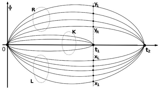
Figure 1: Schematical representation of the directed polymer paths corresponding to eq.(III.1)

III.2 Calculations

Substituting the representations (9) and (8) for the wave functions $\Psi\bigl{(}{\bf x},{\bf 0},{\bf y};\,t\bigr{)}$ and $\Psi^{*}\bigl{(}{\bf x},{\bf y};\,\Delta\,t\bigr{)}$ in eq.(III.1) we obtain:

$$W(f_{1},f_{2},\Delta) = \lim_{t\to\infty}\Biggl{\{}\sum_{L,K,R=0}^{\infty}\frac{(-1)^{L+K+R}}{L!\,K!\,R!}\,\exp\Bigl{[}\lambda_{t}Kf_{1}+(1+\Delta)^{1/3}\lambda_{t}(L+R)f_{2}\Bigr{]}\times$$ (24)

$$\times \int{\cal D}_{Q}\;\int{\cal D}_{P}\;|C({\bf Q})|^{2}|C({\bf P})|^{2}\;\exp\bigl{[}-tE({\bf Q})-\Delta tE({\bf P})\bigr{]}\;I({\bf Q},{\bf P})\Biggr{\}}$$

where

$$I\bigl{(}{\bf Q};{\bf P}\bigr{)} = \sum_{{\cal P}}\;\sum_{\tilde{{\cal P}}}\;\Pi_{LK}({\bf Q})\;\Pi_{LR}({\bf Q})\;\Pi_{KR}({\bf Q})\;\Pi^{*}_{LR}({\bf P})\times$$ (25)

$$\times \int_{-\infty}^{0}dx_{1}...dx_{L}\prod_{1\leq a<b}^{L}\Biggl{[}\Bigl{(}1+i\kappa\frac{\operatorname{sgn}(x_{a}-x_{b})}{Q_{{\cal P}_{a}}-Q_{{\cal P}_{b}}}\Bigr{)}\Bigl{(}1-i\kappa\frac{\operatorname{sgn}(x_{a}-x_{b})}{P_{\tilde{{\cal P}}_{a}}-P_{\tilde{{\cal P}}_{b}}}\Bigr{)}\Biggr{]}\exp\Bigl{[}i\sum_{a=1}^{L}\bigl{(}O_{{\cal P}_{a}}-P_{\tilde{{\cal P}}_{a}}-i\epsilon\bigr{)}x_{a}\Bigr{]}\times$$

$$\times \int_{0}^{+\infty}dy_{R}...dy_{1}\prod_{1\leq c<d}^{R}\Biggl{[}\Bigl{(}1-i\kappa\frac{\operatorname{sgn}(y_{c}-y_{d})}{Q_{{\cal P}_{(L+K+c)}}-Q_{{\cal P}_{(L+K+d)}}}\Bigr{)}\Bigl{(}1+i\kappa\frac{\operatorname{sgn}(y_{c}-y_{d})}{P_{\tilde{{\cal P}}_{(L+c)}}-P_{\tilde{{\cal P}}_{(L+d)}}}\Bigr{)}\Biggr{]}\times$$

$$\times \exp\Bigl{[}i\sum_{c=1}^{R}\bigl{(}Q_{{\cal P}_{(L+K+c)}}-P_{\tilde{{\cal P}}_{(L+c)}}+i\epsilon\bigr{)}y_{c}\Bigr{]}$$

Here, to regularize the integrations at $\pm$ infinities the supplementary factors $\pm i\epsilon$ are introduced (which will be set to zero in the final result). The factors $\Pi_{ij}({\bf Q})\;(i,j=LK,LR,KR)$ and $\Pi^{*}_{LR}({\bf P})$ in the above equation are the cross-products of the prefactors of the type $[1-i\kappa/(Q_{(i)}-Q_{(j)})]$ over the particles belonging to the sectors ”L” and ”K”, ”L” and ”R” and ”K” and ”R” (note that $P_{KK}({\bf Q})\equiv 1$). Correspondingly, $\Pi^{*}_{LR}({\bf P})$ is the cross-product of the prefactors of the type $[1+i\kappa/(P_{(i)}-P_{(j)})]$ over the particles belonging to the sectors ”L” and ”R”.

The summation over all permutations ${\cal P}$ of $(L+K+R)$ momenta $Q_{a}$ over $(L+K+R)$ particles of the sectors ”L” $(x_{1},...,x_{L})$, ”K” (all coordinates equal to zero) and ”R” $(y_{R},...,y_{1})$ can be split into four parts:
(1) the summation over permutations ${\cal P}^{(L)}$ of $L$ (taken at random) momenta $q$ over $L$ particles of the sector ”L”;
(2) the summation over permutations ${\cal P}^{(R)}$ of $R$ (taken at random) momenta $q$ over $R$ particles of the sector ”R”;
(3) the summation over permutations ${\cal P}^{(K)}$ of $K$ remaining momenta $q$ over $K$ particles of the central sector ”K”;
(4) the summation over permutations ${\cal P}^{(LKR)}$ of the momenta $q$ over sectors ”L”, ”K” and ”R”.

Similar splitting can be done for the summation over the permutations $\tilde{{\cal P}}$ of $(L+R)$ momenta $P_{a}$ over $(L+R)$ particles of the sectors ”L” and ”R”. In other words, the summations over the permutations in eq.(25) can be represented as follows:

$$\sum_{{\cal P}}\;\sum_{\tilde{{\cal P}}}\;\Bigl{(}...\Bigr{)}\;=\;\sum_{{\cal P}^{(LKR)}}\sum_{\tilde{{\cal P}}^{(LR)}}\;\sum_{{\cal P}^{(L)}}\;\sum_{\tilde{{\cal P}}^{(L)}}\;\sum_{{\cal P}^{(R)}}\;\sum_{\tilde{{\cal P}}^{(R)}}\;\sum_{{\cal P}^{(K)}}\;\Bigl{(}...\Bigr{)}$$ (26)

To perform the summations over all these permutations we can use the following important property of the Bethe ansatz wave function, eq.(8). Namely, it has such structure that for ordered particle’s positions in the summation over the permutations the momenta components $q^{\alpha}_{r}$ belonging to the same cluster also remain ordered. In other words, if we consider the momenta of a cluster $\alpha$, $\{q^{\alpha}_{1},...,q^{\alpha}_{n_{\alpha}}\}$, eq.(7), belonging correspondingly to the particles $\{x_{i_{1}}<x_{i_{2}}<...<x_{i_{n_{\alpha}}}\}$, the permutation of any two momenta $q^{\alpha}_{r}$ and $q^{\alpha}_{r^{\prime}}$ of this ordered set gives zero contribution. In our case we have three groups of particles: $\{x_{1},...,x_{L}\}\;<\;\{0,...,0\}\;<\;\{y_{R},...,y_{1}\}$. Thus, in order to perform the summation over the permutations ${\cal P}^{(LKR)}$ it is sufficient to split the momenta of each cluster into three parts:

$$\{q^{\alpha}_{1},...,q^{\alpha}_{n_{\alpha}}\}\;\to\;\{q^{\alpha}_{1},...,q^{\alpha}_{m_{\alpha}}\,\big{|}\big{|}\,q^{\alpha}_{m_{\alpha}+1},...,q^{\alpha}_{m_{\alpha}+k_{\alpha}}\,\big{|}\big{|}\,q^{\alpha}_{m_{\alpha}+k_{\alpha}+1},...,q^{\alpha}_{m_{\alpha}+k_{\alpha}+s_{\alpha}}\}$$ (27)

defined by three integer parameters $m_{\alpha},k_{\alpha}$ and $s_{\alpha}$, such that $m_{\alpha}+k_{\alpha}+s_{\alpha}=n_{\alpha}$. In such cluster structure the momenta components of the left group $\{q^{\alpha}_{1},...,q^{\alpha}_{m_{\alpha}}\}$ go to the particles of the sector ”L”; the momenta components of the central group $\{q^{\alpha}_{m_{\alpha}+1},...,q^{\alpha}_{m_{\alpha}+k_{\alpha}}\}$ go to the particles of the sector ”K”; and the momenta components of the right group $\{q^{\alpha}_{m_{\alpha}+k_{\alpha}+1},...,q^{\alpha}_{m_{\alpha}+k_{\alpha}+s_{\alpha}}\}$ go to the particles of the sector ”R”.

Similarly, to perform the summation over the permutations $\tilde{{\cal P}}^{(LR)}$ of the momenta $p^{\alpha}_{r}$ each cluster is split into two parts: $\{p^{\alpha}_{1},...,p^{\alpha}_{m_{\alpha}}\,\big{|}\big{|}\,p^{\alpha}_{m_{\alpha}+1},...,p^{\alpha}_{m_{\alpha}+s_{\alpha}}\}$. Here the components $\{p^{\alpha}_{1},...,p^{\alpha}_{m_{\alpha}}\}$ go to the particle of the sector ”L”, while the components $\{p^{\alpha}_{m_{\alpha}+1},...,p^{\alpha}_{m_{\alpha}+s_{\alpha}}\}$ go to the particle of the sector ”R”. In this way, the summations over the permutations ${\cal P}^{(LKR)}$ and $\tilde{{\cal P}}^{(LR)}$ is changed by the summations over the integer parameters $\{m_{\alpha},k_{\alpha},s_{\alpha}\}$ constrained by the conditions:

$$\sum_{\alpha=1}^{M}\;m_{\alpha}=L\,,\;\;\;\;\;\;\;\sum_{\alpha=1}^{M}\;k_{\alpha}=K\,,\;\;\;\;\;\;\;\sum_{\alpha=1}^{M}\;s_{\alpha}=R$$ (28)

Performing simple integrations over $x_{1},...,x_{L}$ and $y_{R},...,y_{1}$ in eq.(25) and taking into account that all cross-product factors $\Pi_{ij}$ are symmetric with respect to the permutations ${\cal P}^{(L)},{\cal P}^{(K)},{\cal P}^{(R)},\tilde{{\cal P}}^{(L)}$ and $\tilde{{\cal P}}^{(R)}$, we get:

$$I({\bf Q},{\bf P})=L!\,K!\,R!\prod_{\alpha=1}^{M}\Biggl{[}\sum_{m_{\alpha}+k_{\alpha}+s_{\alpha}\geq 1}\Biggr{]}\delta_{\sum m_{\alpha},L}\;\delta_{\sum k_{\alpha},K}\;\delta_{\sum s_{\alpha},R}\;{\cal G}\bigl{(}{\bf Q},{\bf P}\bigr{)}\;D_{L}({\bf Q},{\bf P})\,D_{R}({\bf Q},{\bf P})$$ (29)

where $\delta_{i,j}$ is the kronecker symbol,

$${\cal G}\bigl{(}{\bf Q},{\bf P}\bigr{)}=\Pi_{LK}\bigl{(}{\bf Q}\bigr{)}\;\Pi_{LR}\bigl{(}{\bf Q}\bigr{)}\;\Pi_{KR}\bigl{(}{\bf Q}\bigr{)}\;\Pi^{*}_{LR}\bigl{(}{\bf P}\bigr{)}$$ (30)

and

$$D_{L}({\bf Q},{\bf P})=\sum_{{\cal P}^{(L)}}\sum_{\tilde{{\cal P}}^{(L)}}\frac{1}{\prod_{a=1}^{L}\Bigl{[}\sum_{b=1}^{a}\bigl{(}Q_{{\cal P}^{(L)}_{b}}-P_{\tilde{{\cal P}}^{(L)}_{b}}-i\epsilon\bigr{)}\Bigr{]}}\prod_{1\leq a<b}^{L}\Biggl{[}\Bigl{(}1-\frac{i\kappa}{Q_{{\cal P}^{(L)}_{a}}-Q_{{\cal P}^{(L)}_{b}}}\Bigr{)}\Bigl{(}1+\frac{i\kappa}{P_{\tilde{{\cal P}}^{(L)}_{a}}-P_{\tilde{{\cal P}}^{(L)}_{b}}}\Bigr{)}\Biggr{]}$$ (31)

$$D_{R}({\bf Q},{\bf P}) = \sum_{{\cal P}^{(R)}}\sum_{\tilde{{\cal P}}^{(R)}}\frac{1}{\prod_{a=L+K+R}^{L+K+1}\Bigl{[}\sum_{b=L+K+R}^{a}\bigl{(}Q^{*}_{{\cal P}^{(L)}_{b}}-P^{*}_{\tilde{{\cal P}}^{(L)}_{b}}+i\epsilon\bigr{)}\Bigr{]}}\times$$ (32)

$$\times \prod_{L+K+1\leq a<b}^{L+K+R}\Biggl{[}\Bigl{(}1+\frac{i\kappa}{Q^{*}_{{\cal P}^{(L)}_{a}}-Q^{*}_{{\cal P}^{(L)}_{b}}}\Bigr{)}\Bigl{(}1-\frac{i\kappa}{P^{*}_{\tilde{{\cal P}}^{(L)}_{a}}-P^{*}_{\tilde{{\cal P}}^{(L)}_{b}}}\Bigr{)}\Biggr{]}$$

Here the momenta components in the ”L” sector are

$$Q_{a} \equiv q^{\alpha}_{r}=q_{\alpha}-\frac{1}{2}i\kappa\bigl{(}m_{\alpha}+k_{\alpha}+s_{\alpha}+1-2r\bigr{)}$$

$$P_{a} \equiv p^{\alpha}_{r}=p_{\alpha}+\frac{1}{2}i\kappa\bigl{(}m_{\alpha}+s_{\alpha}+1-2r\bigr{)}$$

with $r=1,...,m_{\alpha}$, while in the ”R” sector the momenta components are counted ”backwards” which makes them complex conjugate:

$$Q^{*}_{a} \equiv {q^{*}}^{\alpha}_{r}=q_{\alpha}+\frac{1}{2}i\kappa\bigl{(}m_{\alpha}+k_{\alpha}+s_{\alpha}+1-2r\bigr{)}$$

$$P^{*}_{a} \equiv {p^{*}}^{\alpha}_{r}=p_{\alpha}-\frac{1}{2}i\kappa\bigl{(}m_{\alpha}+s_{\alpha}+1-2r\bigr{)}$$

with $r=1,...,s_{\alpha}$. It turs out that the factors $D_{L}({\bf Q},{\bf P})$ and $D_{R}({\bf Q},{\bf P})$, eqs(31)-(32), can be nicely represented in the determinant form Gauden :

$$D_{L}({\bf Q},{\bf P})=\delta_{L}^{-1}({\bf Q},{\bf P})\;\det\Bigl{[}\frac{1}{(Q_{a}-P_{b}-i\epsilon)(Q_{a}-P_{b}-i\epsilon+i\kappa)}\Bigr{]}_{a,b=1,..,L}$$ (35)

where

$$\delta_{L}({\bf Q},{\bf P})=\det\Bigl{[}\frac{1}{Q_{a}-P_{b}-i\epsilon+i\kappa}\Bigr{]}_{a,b=1,..,L}=\frac{\prod_{1\leq a<b}^{L}\bigl{[}(Q_{a}-Q_{b})(P_{a}-P_{b})\bigr{]}}{\prod_{a,b=1}^{L}\bigl{(}Q_{a}-P_{b}-i\epsilon+i\kappa\bigr{)}}$$ (36)

The expression for $D_{R}({\bf Q},{\bf P})$ is obtained from eqs.(35)-(36) by changing $Q_{a}\to Q^{*}_{a}$, $P_{a}\to P^{*}_{a}$ and $L\to R$.

Thus, substituting eqs.(29), (10) and (11) into eq.(24) and taking into account that the wave function $\Psi_{\bf P}({\bf x},{\bf y})$ exists only provided $(m_{\alpha}+s_{\alpha})\geq 1$ we get:

$$W(f_{1},f_{2},\Delta) = 1+\lim_{t\to\infty}\sum_{M=1}^{\infty}\frac{(-1)^{M}}{M!}\prod_{\alpha=1}^{M}\Biggl{[}\int_{-\infty}^{+\infty}\frac{dq_{\alpha}}{2\pi}\Biggr{]}\sum_{M_{1}=0}^{M}\frac{1}{M_{1}!}\prod_{\beta=1}^{M_{1}}\Biggl{[}\int_{-\infty}^{+\infty}\frac{dp_{\beta}}{2\pi}\Biggr{]}\times$$ (37)

$$\times \frac{M!}{M_{1}!(M-M_{1})!}\;\prod_{\beta=1}^{M_{1}}\Biggl{[}\sum_{k_{\beta}=0}^{\infty}\sum_{m_{\beta}+s_{\beta}\geq 1}^{\infty}(-1)^{m_{\beta}+k_{\beta}+s_{\beta}-1}\Biggr{]}\prod_{\gamma=M_{1}+1}^{M}\Biggl{[}\sum_{k_{\gamma}=1}^{\infty}\delta_{m_{\gamma},0}\;\delta_{s_{\gamma},0}(-1)^{k_{\gamma}-1}\Biggr{]}\times$$

$$\times \exp\Biggl{\{}\sum_{\alpha=1}^{M}\Bigl{[}\lambda_{t}k_{\alpha}f_{1}+(1+\Delta)^{1/3}\lambda_{t}(m_{\alpha}+s_{\alpha})f_{2}-tE(q_{\alpha},m_{\alpha}+k_{\alpha}+s_{\alpha})\Bigr{]}-\Delta\,t\sum_{\beta=1}^{M_{1}}E(p_{\beta},m_{\beta}+s_{\beta})\Biggr{\}}\times$$

$$\times \det\Biggl{[}\frac{1}{\frac{1}{2}\kappa(m_{\alpha}+k_{\alpha}+s_{\alpha})-iq_{\alpha}+\frac{1}{2}\kappa(m_{\alpha^{\prime}}+k_{\alpha^{\prime}}+s_{\alpha^{\prime}})+iq_{\alpha^{\prime}}}\Biggr{]}_{\alpha,\alpha^{\prime}=1,...,M}\;\times$$

$$\times \det\Biggl{[}\frac{1}{\frac{1}{2}\kappa(m_{\beta}+s_{\beta})+ip_{\beta}+\frac{1}{2}\kappa(m_{\beta^{\prime}}+s_{\beta^{\prime}})-ip_{\beta^{\prime}}}\Biggr{]}_{\beta,\beta^{\prime}=1,...,M_{1}}\;\times$$

$$\times D_{L}\bigl{(}{\bf q},{\bf p},{\bf m},{\bf k},{\bf s}\bigr{)}\;D_{R}\bigl{(}{\bf q},{\bf p},{\bf m},{\bf k},{\bf s}\bigr{)}\;{\cal G}\bigl{(}{\bf q},{\bf p},{\bf m},{\bf k},{\bf s}\bigr{)}$$

where

$$E(q,n)\;=\;\frac{1}{2\beta}nq^{2}-\frac{\kappa^{2}}{24\beta}n^{3}$$ (38)

and instead of the vectors ${\bf Q}$ and ${\bf P}$ in the arguments of the functions $D_{L}$, $D_{R}$ and ${\cal G}$ we have introduced the vectors ${\bf q}=\{q_{1},...,q_{M}\}$, ${\bf p}=\{p_{1},...,p_{M_{1}}\}$, ${\bf m}=\{m_{1},...,m_{M}\}$, ${\bf k}=\{k_{1},...,k_{M}\}$ and ${\bf s}=\{s_{1},...,s_{M}\}$.

Now using explicit expressions for the momenta components $q^{\alpha}_{r}$ and $p^{\alpha}_{r}$, eqs.(LABEL:32)-(LABEL:33), we have to express the factors $D_{L}$, $D_{R}$, eqs.(35)-(36), and ${\cal G}$, eq.(30), in terms of analytic functions of the parameters $q_{\alpha},p_{\alpha},m_{\alpha},k_{\alpha}$ and $s_{\alpha}$. One can easily note that due to the symmetry of the expressions (37) and (35)-(36) with respect to permutations of the clusters, the factors $D_{L}$ and $D_{R}$ in eq.(37) can be represented as follows:

$$D_{L} = \frac{L!}{\prod_{\alpha=1}^{M}m_{\alpha}!}\;\delta_{L}^{-1}\;\prod_{\alpha=1}^{M}d_{\alpha}^{(L)}$$ (39)

$$D_{R} = \frac{R!}{\prod_{\alpha=1}^{M}s_{\alpha}!}\;\delta_{R}^{-1}\;\prod_{\alpha=1}^{M}d_{\alpha}^{(R)}$$ (40)

where

$$d_{\alpha}^{(L)} = \det\Bigl{[}\frac{1}{\bigl{(}q^{\alpha}_{r}-p^{\alpha}_{r^{\prime}}-i\epsilon\bigr{)}\bigl{(}q^{\alpha}_{r}-p^{\alpha}_{r^{\prime}}-i\epsilon+i\kappa\bigr{)}}\Bigr{]}_{r,r^{\prime}=1,...,m_{\alpha}}$$ (41)

$$d_{\alpha}^{(R)} = \det\Bigl{[}\frac{1}{\bigl{(}{q^{*}}^{\alpha}_{r}-{p^{*}}^{\alpha}_{r^{\prime}}+i\epsilon\bigr{)}\bigl{(}{q^{*}}^{\alpha}_{r}-{p^{*}}^{\alpha}_{r^{\prime}}+i\epsilon-i\kappa\bigr{)}}\Bigr{]}_{r,r^{\prime}=1,...,s_{\alpha}}$$ (42)

Using eq.(LABEL:32) the determinant (41) can be represented as follows:

$$d_{\alpha}^{(L)}\;=\;(i\kappa)^{-m_{\alpha}}\;\det\Bigl{[}\frac{1}{(x_{\alpha}+r+r^{\prime}-2)(x_{\alpha}+r+r^{\prime}-1)}\Bigr{]}_{r,r^{\prime}=1,...,m_{\alpha}}$$ (43)

where

$$x_{\alpha}=-iA_{\alpha}^{(-)}-m_{\alpha}-s_{\alpha}-\frac{1}{2}k_{\alpha}+1$$ (44)

and

$$A_{\alpha}^{(-)}=\frac{1}{\kappa}(q_{\alpha}-p_{\alpha})-i\epsilon$$ (45)

Sufficiently simple calculations yield:

$$d_{\alpha}^{(L)}\;=\;(i\kappa)^{-m_{\alpha}}\;\frac{m_{\alpha}!\prod_{l=1}^{m_{\alpha}}l^{2(m_{\alpha}-l)}}{\prod_{l=1}^{m_{\alpha}}\Bigl{[}(x_{\alpha}+l-1)^{l}(x_{\alpha}+2m_{\alpha}-l)^{l}\Bigr{]}}$$ (46)

The expression for $D_{\alpha}^{(R)}$ is obtained from eqs.(41) and (46) by changing $m_{\alpha}\to s_{\alpha}$ and $iA_{\alpha}^{(-)}\to-iA_{\alpha}^{(+)}$.

After somewhat painful algebra for the factor $\delta_{L}^{-1}$ one obtains the following expression:

$$\delta_{L}^{-1}=(i\kappa)^{L}\frac{\prod_{\alpha=1}^{M}\prod_{r,r^{\prime}=1}^{m_{\alpha}}\Bigl{[}-iA_{\alpha}^{(-)}-n_{\alpha}-\frac{1}{2}k_{\alpha}+r+r^{\prime}\Bigr{]}\;\prod_{\alpha\not=\beta}^{M}\prod_{r=1}^{m_{\alpha}}\prod_{r^{\prime}=1}^{m_{\beta}}\Bigl{[}R_{\alpha\beta}+r+r^{\prime}\Bigr{]}}{\prod_{\alpha=1}^{M}\prod_{1\leq r<r^{\prime}}^{m_{\alpha}}(r-r^{\prime})^{2}\;\prod_{1\leq\alpha<\beta}^{M}\prod_{r=1}^{m_{\alpha}}\prod_{r^{\prime}=1}^{m_{\beta}}\Bigl{[}\bigl{(}Q_{\alpha\beta}+r-r^{\prime}\bigr{)}\bigl{(}P_{\alpha\beta}+r-r^{\prime}\bigr{)}\Bigr{]}}$$ (47)

where

$$Q_{\alpha\beta} = -\frac{i}{\kappa}(q_{\alpha}-q_{\beta})-\frac{1}{2}(n_{\alpha}^{\prime}-n_{\beta}^{\prime})$$

$$P_{\alpha\beta} = \frac{i}{\kappa}(p_{\alpha}-p_{\beta})-\frac{1}{2}(n_{\alpha}-n_{\beta})$$ (48)

$$R_{\alpha\beta} = -\frac{i}{\kappa}(q_{\alpha}-p_{\beta})-\frac{1}{2}(n_{\alpha}^{\prime}-n_{\beta})$$

and

$$n_{\alpha} = m_{\alpha}+s_{\alpha}$$

$$n_{\alpha}^{\prime} = m_{\alpha}+s_{\alpha}+k_{\alpha}$$

Using the properties of the Barnes $G$-function:

$$G(N+1) = \prod_{l=1}^{N}\Gamma(l)$$

$$G(z+1) = \Gamma(z)G(z)$$

(50)

$$\prod_{l=1}^{N}\Gamma(z+l) = \frac{G(z+N+1)}{G(z+1)}$$

$$\prod_{l=1}^{N}(z+l)^{l} = \Gamma^{N}(z+N+1)\,\frac{G(z+1)}{G(z+N+1)}$$

for the factors (46) and (47) one eventually obtains the following expressions:

$$d_{\alpha}^{(L)} = (i\kappa)^{-m_{\alpha}}\;\frac{\Gamma(m_{\alpha}+1)G^{2}(m_{\alpha}+1)G(n_{\alpha}+\frac{1}{2}k_{\alpha}-m_{\alpha}+iA_{\alpha}^{(-)}+1)}{G(n_{\alpha}+\frac{1}{2}k_{\alpha}+iA_{\alpha}^{(-)}+1)}\times\frac{G(n_{\alpha}+\frac{1}{2}k_{\alpha}-m_{\alpha}+iA_{\alpha}^{(-)})}{G(n_{\alpha}+\frac{1}{2}k_{\alpha}-2m_{\alpha}+iA_{\alpha}^{(-)})}$$ (51)

$$\delta_{L}^{-1} = \prod_{\alpha=1}^{M}\Biggl{[}\frac{(i\kappa)^{-m_{\alpha}}G(n_{\alpha}+\frac{1}{2}k_{\alpha}+iA_{\alpha}^{(-)})G(n_{\alpha}+\frac{1}{2}k_{\alpha}-2m_{\alpha}+iA_{\alpha}^{(-)})}{G^{2}(m_{\alpha}+1)G^{2}(n_{\alpha}+\frac{1}{2}k_{\alpha}-m_{\alpha}+iA_{\alpha}^{(-)})}\Biggr{]}\times\prod_{\alpha\not=\beta}^{M}{\cal B}_{\alpha\beta}^{(L)}$$ (52)

where

$${\cal B}_{\alpha\beta}^{(L)} = \frac{G(Q_{\alpha\beta}+1)G(P_{\alpha\beta}+1)G(Q_{\alpha\beta}+m_{\alpha}-m_{\beta}+1)G(P_{\alpha\beta}-m_{\alpha}+m_{\beta}+1)}{G(Q_{\alpha\beta}+m_{\alpha}+1)G(P_{\alpha\beta}-m_{\alpha}+1)G(Q_{\alpha\beta}-m_{\beta}+1)G(P_{\alpha\beta}+m_{\beta}+1)}\times$$

$$\times \frac{G(R_{\alpha\beta}+m_{\alpha}+m_{\beta}+2)G(R_{\beta\alpha}+m_{\alpha}+m_{\beta}+2)G(R_{\alpha\beta}+2)G(R_{\beta\alpha}+2)}{G(R_{\alpha\beta}+m_{\alpha}+2)G(R_{\beta\alpha}+m_{\beta}+2)G(R_{\alpha\beta}+m_{\beta}+2)G(R_{\beta\alpha}+m_{\alpha}+2)}$$

Finally, substituting eqs.(51) and (52) into eq.(39) we get:

$$D_{L}=\Gamma\bigl{(}\sum_{\alpha}m_{\alpha}+1\bigr{)}\prod_{\alpha=1}^{M}\Biggl{[}\frac{G(n_{\alpha}+\frac{1}{2}k_{\alpha}-m_{\alpha}+iA_{\alpha}^{(-)}+1)G(n_{\alpha}+\frac{1}{2}k_{\alpha}+iA_{\alpha}^{(-)})}{G(n_{\alpha}+\frac{1}{2}k_{\alpha}+iA_{\alpha}^{(-)}+1)G(n_{\alpha}+\frac{1}{2}k_{\alpha}-m_{\alpha}+iA_{\alpha}^{(-)})}\Biggr{]}\times\prod_{\alpha\not=\beta}^{M}{\cal B}_{\alpha\beta}^{(L)}$$ (54)

The expression for $D_{R}$ is obtained from eq.(54) by changing $m_{\alpha}\to s_{\alpha}$ and $iA_{\alpha}^{(-)}\to-iA_{\alpha}^{(+)}$. In the similar way one can derive the analytic expression for the cross-product factor ${\cal G}$, eq.(30). The final formula for this factor is rather cumbersome: it contains the products of all kinds of Gamma functions of the type $\Gamma\bigl{[}1+\frac{1}{2}(\pm m_{\alpha}\pm s_{\alpha}\pm k_{\alpha}\pm m_{\beta}\pm s_{\beta}\pm k_{\beta})\pm i(q_{\alpha}-q_{\beta})/\kappa\bigr{]}$ and $\Gamma\bigl{[}1+\frac{1}{2}(\pm m_{\alpha}\pm s_{\alpha}\pm m_{\beta}\pm s_{\beta})\pm i(p_{\alpha}-p_{\beta})/\kappa\bigr{]}$ (the example of such type of product one can see in end-point , eq.(A.17)). We do not reproduce it here as it turns out to be irrelevant in the limit $t\to\infty$ (see below).

III.3 Thermodynamic limit $t\to\infty$

Next step of the calculations is to take the limit $t\to\infty$ and to perform the summations over the integers $m_{\alpha},s_{\alpha}$ and $k_{\alpha}$ After rescaling

$$q_{\alpha} \to \frac{\kappa}{2\lambda_{t}}\,q_{\alpha}$$

$$p_{\alpha} \to \frac{\kappa}{2\lambda_{t}}\,p_{\alpha}$$

with

$$\lambda_{t}\;=\;\frac{1}{2}\Bigl{(}\frac{\kappa^{2}t}{\beta}\Bigr{)}^{1/3}\;=\;\frac{1}{2}\bigl{(}\beta^{5}u^{2}t\bigr{)}^{1/3}$$ (56)

the expression for the probability distribution function $W(f_{1},f_{2},\Delta)$, eq.(37), reduces to

$$W(f_{1},f_{2},\Delta) = 1+\lim_{\lambda_{t}\to\infty}\sum_{M=1}^{\infty}\sum_{M_{1}=1}^{M}\frac{(-1)^{M}}{(M_{1}!)^{2}(M-M_{1})!}\times$$ (57)

$$\times \prod_{\beta=1}^{M_{1}}\Biggl{[}\int\int_{-\infty}^{+\infty}\frac{dq_{\beta}dp_{\beta}}{(2\pi)^{2}}\sum_{k_{\beta}=0}^{\infty}\sum_{m_{\beta}+s_{\beta}\geq 1}^{\infty}(-1)^{m_{\beta}+k_{\beta}+s_{\beta}-1}\times$$

$$\times \exp\Bigl{\{}\lambda_{t}k_{\beta}f_{1}+(1+\Delta)^{1/3}\lambda_{t}(m_{\beta}+s_{\beta})f_{2}-\lambda(m_{\beta}+k_{\beta}+s_{\beta})q_{\beta}^{2}+\frac{1}{3}\lambda_{t}^{3}(m_{\beta}+k_{\beta}+s_{\beta})^{3}$$

$$- \Delta\,\lambda_{t}(m_{\beta}+s_{\beta})p_{\beta}^{2}+\frac{1}{3}\Delta\,\lambda_{t}^{3}(m_{\beta}+s_{\beta})^{3}\Bigr{\}}\;J\Bigl{(}\frac{q_{\beta}-p_{\beta}}{\lambda_{t}},m_{\beta},s_{\beta},k_{\beta}\Bigr{)}\Biggr{]}\times$$

$$\times \prod_{\gamma=M_{1}+1}^{M}\Biggl{[}\int_{-\infty}^{+\infty}\frac{dq_{\gamma}}{2\pi}\sum_{k_{\gamma}=1}^{\infty}\delta_{m_{\gamma},0}\;\delta_{s_{\gamma},0}(-1)^{k_{\gamma}-1}\exp\Bigl{\{}\lambda_{t}k_{\gamma}f_{1}-\lambda_{t}k_{\gamma}q_{\gamma}^{2}+\frac{1}{3}\lambda_{t}^{3}k_{\gamma}^{3}\Bigr{\}}\Biggr{]}\times$$

$$\times \det\Biggl{[}\frac{1}{\lambda_{t}(m_{\alpha}+k_{\alpha}+s_{\alpha})-iq_{\alpha}+\lambda_{t}(m_{\alpha^{\prime}}+k_{\alpha^{\prime}}+s_{\alpha^{\prime}})+iq_{\alpha^{\prime}}}\Biggr{]}_{\alpha,\alpha^{\prime}=1,...,M}\;\times$$

$$\times \det\Biggl{[}\frac{1}{\lambda_{t}(m_{\beta}+s_{\beta})+ip_{\beta}+\lambda_{t}(m_{\beta^{\prime}}+s_{\beta^{\prime}})-ip_{\beta^{\prime}}}\Biggr{]}_{\beta,\beta^{\prime}=1,...,M_{1}}\;\times$$

$$\times \prod_{\alpha\not=\alpha^{\prime}}^{M}\Bigl{[}{\cal B}_{\alpha\alpha^{\prime}}^{(L)}{\cal B}_{\alpha\alpha^{\prime}}^{(R)}\Bigr{]}\;{\cal G}\Biggr{\}}$$

Here

$$J\Bigl{(}\frac{q-p}{\lambda_{t}},m,s,k\Bigr{)} = \Gamma(m+1)\Gamma(s+1)\times$$ (58)

$$\times \frac{G\bigl{(}n+\frac{1}{2}k-m+\frac{i}{2\lambda_{t}}(q-p)^{(-)}+1\bigr{)}G\bigl{(}n+\frac{1}{2}k-s-\frac{i}{2\lambda_{t}}(q-p)^{(+)}+1\bigr{)}}{G\bigl{(}n+\frac{1}{2}k+\frac{i}{2\lambda_{t}}(q-p)^{(-)}+1\bigr{)}G\bigl{(}n+\frac{1}{2}k-\frac{i}{2\lambda_{t}}(q-p)^{(+)}+1\bigr{)}}\times$$

$$\times \frac{G\bigl{(}n+\frac{1}{2}k+\frac{i}{2\lambda_{t}}(q-p)^{(-)}\bigr{)}G\bigl{(}n+\frac{1}{2}k-\frac{i}{2\lambda_{t}}(q-p)^{(+)}\bigr{)}}{G\bigl{(}n+\frac{1}{2}k-m+\frac{i}{2\lambda_{t}}(q-p)^{(-)}\bigr{)}G\bigl{(}n+\frac{1}{2}k-s-\frac{i}{2\lambda_{t}}(q-p)^{(+)}\bigr{)}}$$

where $n=m+s$ and $(q-p)^{(\pm)}\;\equiv\;q-p\pm i\epsilon$.

The summations over the integers $m_{\alpha},s_{\alpha}$ and $k_{\alpha}$ in the limit $\lambda\to\infty$ is performed according to the following heuristic algorithm (see also goe ; end-point ). Let us consider the example of the series of a general type:

$$R=\lim_{\lambda\to\infty}\;\prod_{\alpha=1}^{M}\Biggl{[}\sum_{n_{\alpha}=0}^{\infty}(-1)^{n_{\alpha}-1}\Biggr{]}\;\Phi\bigl{(}\lambda;\,\lambda{\bf n};\,{\bf n}\bigr{)}$$ (59)

where $\Phi\bigl{(}\lambda;\,\lambda z_{1},...,\lambda z_{M};\,z_{1},...,z_{M}\bigr{)}$ as a function of the variables $\{z_{1},...,z_{M}\}$ has ”good” analytic properties in the complex half-plane, $\mbox{Re}(z_{\alpha})\geq 0$. Then the summations in the above equation can be represented in terms of the following contour integrals:

$$R=\lim_{\lambda\to\infty}\;\prod_{\alpha=1}^{M}\Biggl{[}\frac{1}{2i}\int_{{\cal C}}\frac{dz_{\alpha}}{\sin(\pi z_{\alpha})}\Biggr{]}\;\Phi\bigl{(}\lambda;\,\lambda{\bf z};\,{\bf z}\bigr{)}$$ (60)

where the integration contour ${\cal C}$ is shown in Figure 2a. After rescaling, $z_{\alpha}\to z_{\alpha}/\lambda$ we get:

$$R=\;\prod_{\alpha=1}^{M}\Biggl{[}\frac{1}{2\pi i}\int_{{\cal C}}\frac{dz_{\alpha}}{z_{\alpha}}\Biggr{]}\;\lim_{\lambda\to\infty}\;\Phi\bigl{(}\lambda;\,{\bf z};\,{\bf z}/\lambda\bigr{)}$$ (61)

where the parameters $z_{\alpha}$ remain finite in the limit $\lambda\to\infty$. Note that if the summation in eq.(59) starts at $n=1$ (and not at $n=0$), the integration in eq.(61) goes along the contour ${\cal C}^{\prime}$ shown in Figure 2b.

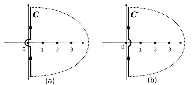
Figure 2: (a) Contour of integration ${\cal C}$ in eq.(60); (b) Contour of integration ${\cal C}^{\prime}$ in the case the summation of the series (59) starts at $n=1$

Applying the above algorithm for the expression in eq.(57) and taking into account that

$$\lim_{|z|\to 0}\;\Gamma(z+1) = 1$$

$$\lim_{|z|\to 0}\;G(z+1) = 1$$ (62)

$$G(z)\big{|}_{|z|\ll 1} \simeq z$$

we find:

$$\lim_{\lambda_{t}\to\infty}\;{\cal B}_{\alpha\beta}^{(L,R)} = 1$$

$$\lim_{\lambda_{t}\to\infty}\;{\cal G} = 1$$

and

$$\lim_{\lambda_{t}\to\infty}\;J\Bigl{(}\frac{q-p}{\lambda_{t}},\frac{z_{1}}{\lambda_{t}},\frac{z_{2}}{\lambda_{t}},\frac{z_{3}}{\lambda_{t}}\Bigr{)}=\Biggl{(}1+\frac{z_{1}}{z_{2}+\frac{1}{2}z_{3}+\frac{1}{2}i(q-p)^{(-)}}\Biggr{)}\Biggl{(}1+\frac{z_{2}}{z_{1}+\frac{1}{2}z_{3}-\frac{1}{2}i(q-p)^{(+)}}\Biggr{)}\equiv J_{*}\bigl{(}q-p,z_{1},z_{2},z_{3}\bigr{)}$$ (64)

Thus, instead of eq.(57), in the limit $\lambda_{t}\to\infty$ we get the following much more simple expression:

$$W(f_{1},f_{2},\Delta) = 1+\sum_{M=1}^{\infty}\sum_{M_{1}=1}^{M}\frac{(-1)^{M}}{(M_{1}!)^{2}(M-M_{1})!}$$ (65)

$$\times \prod_{\beta=1}^{M_{1}}\Biggl{[}\int\int_{-\infty}^{+\infty}\frac{dq_{\beta}dp_{\beta}}{(2\pi)^{2}}\int\int_{-\infty}^{+\infty}\frac{dy_{1}dy_{2}}{\Delta^{1/3}}\operatorname{Ai}\bigl{(}y_{1}+q_{\beta}^{2}-f_{1}\bigr{)}\operatorname{Ai}\Bigl{(}\frac{y_{2}+\Delta\,p_{\beta}^{2}-(1+\Delta)^{1/3}f_{2}+f_{1}}{\Delta^{1/3}}\Bigr{)}\times$$

$$\times \int_{{\cal C}}\frac{d{z_{3}}_{\beta}}{{z_{3}}_{\beta}}\int_{{\cal C}}d{z_{1}}_{\beta}\int_{{\cal C}}d{z_{2}}_{\beta}\Bigl{(}\frac{1}{{z_{1}}_{\beta}{z_{2}}_{\beta}}-\delta({z_{1}}_{\beta})\delta({z_{2}}_{\beta})\Bigr{)}J_{*}\Bigl{(}q_{\beta}-p_{\beta},{z_{1}}_{\beta},{z_{2}}_{\beta},{z_{3}}_{\beta}\Bigr{)}\times$$

$$\times \exp\bigl{\{}({z_{1}}_{\beta}+{z_{2}}_{\beta})(y_{1}+y_{2})+{z_{3}}_{\beta}y_{1}\bigr{\}}\Biggr{]}\times$$

$$\times \prod_{\gamma=M_{1}+1}^{M}\Biggl{[}\int\int_{-\infty}^{+\infty}\frac{dq_{\gamma}dy_{1}}{2\pi}\operatorname{Ai}\bigl{(}y_{1}+q_{\gamma}^{2}-f_{1}\bigr{)}\int_{{\cal C}^{\prime}}\frac{d{z_{3}}_{\gamma}}{{z_{3}}_{\gamma}}\int_{{\cal C}}d{z_{1}}_{\gamma}\int_{{\cal C}}d{z_{2}}_{\gamma}\delta({z_{1}}_{\gamma})\delta({z_{2}}_{\gamma})\exp\bigl{\{}{z_{3}}_{\gamma}y_{1}\bigr{\}}\Biggr{]}\times$$

$$\times \det\Biggl{[}\frac{1}{{z_{1}}_{\alpha}+{z_{2}}_{\alpha}+{z_{3}}_{\alpha}-iq_{\alpha}+{z_{1}}_{\alpha^{\prime}}+{z_{2}}_{\alpha^{\prime}}+{z_{3}}_{\alpha^{\prime}}+iq_{\alpha^{\prime}}}\Biggr{]}_{\alpha,\alpha^{\prime}=1,...,M}\times$$

$$\times \det\Biggl{[}\frac{1}{{z_{1}}_{\beta}+{z_{2}}_{\beta}+ip_{\beta}+{z_{1}}_{\beta^{\prime}}+{z_{2}}_{\beta^{\prime}}-ip_{\beta^{\prime}}}\Biggr{]}_{\beta,\beta^{\prime}=1,...,M_{1}}$$

where we have used the Airy function identity

$$\exp\Bigl{\{}\frac{1}{3}z^{3}\Bigr{\}}\;=\;\int_{-\infty}^{+\infty}dy\;\operatorname{Ai}(y)\;\exp\bigl{\{}zy\bigr{\}}$$ (66)

III.4 The Result

One can easily see that the expression for the function $W(f_{1},f_{2},\Delta)$, eq.(65), is not the Fredholm determinant. Consequently, it can not be represented in the exponential form in terms of the trace of the corresponding matrix which was the standard step in all previous Bethe ansatz replica calculations of the Fredholm determinant integral kernels (see e.g. BA-TW2 ; LeDoussal1 ; rev-TW ). Nevertheless, sufficiently simple structure of two determinants in eq.(65) allows to perform significant simplification of this expression.

Indeed, for the first $M\times M$ determinant in eq.(65) we have:

$$\mbox{det}_{M} \equiv \det\Biggl{[}\frac{1}{{z_{1}}_{\alpha}+{z_{2}}_{\alpha}+{z_{3}}_{\alpha}-iq_{\alpha}+{z_{1}}_{\alpha^{\prime}}+{z_{2}}_{\alpha^{\prime}}+{z_{3}}_{\alpha^{\prime}}+iq_{\alpha^{\prime}}}\Biggr{]}_{\alpha,\alpha^{\prime}=1,...,M}$$ (67)

$$= \sum_{{\cal P}\in S_{M}}(-1)^{\bigl{[}{\cal P}\bigr{]}}\prod_{\alpha=1}^{M}\bigl{(}{z_{1}}_{\alpha}+{z_{2}}_{\alpha}+{z_{3}}_{\alpha}-iq_{\alpha}+{z_{1}}_{{\cal P}_{\alpha}}+{z_{2}}_{{\cal P}_{\alpha}}+{z_{3}}_{{\cal P}_{\alpha}}+iq_{{\cal P}_{\alpha}}\bigr{)}^{-1}$$

$$= \prod_{\alpha=1}^{M}\Biggl{[}\int_{0}^{\infty}du_{\alpha}\Biggr{]}\sum_{{\cal P}\in S_{M}}(-1)^{\bigl{[}{\cal P}\bigr{]}}\exp\Bigl{\{}-\sum_{\alpha=1}^{M}\bigl{(}{z_{1}}_{\alpha}+{z_{2}}_{\alpha}+{z_{3}}_{\alpha}\bigr{)}u_{\alpha}-\sum_{\alpha=1}^{M}\bigl{(}{z_{1}}_{{\cal P}_{\alpha}}+{z_{2}}_{{\cal P}_{\alpha}}+{z_{3}}_{{\cal P}_{\alpha}}\bigr{)}u_{\alpha}\Bigr{\}}\times$$

$$\times \exp\Bigl{\{}-\sum_{\alpha=1}^{M}q_{\alpha}u_{\alpha}-\sum_{\alpha=1}^{M}q_{{\cal P}_{\alpha}}u_{\alpha}\Bigr{\}}$$

Since

$$\sum_{\alpha=1}^{M}\bigl{(}{z_{1}}_{{\cal P}_{\alpha}}+{z_{2}}_{{\cal P}_{\alpha}}+{z_{3}}_{{\cal P}_{\alpha}}\bigr{)}u_{\alpha}\;=\;\sum_{\alpha=1}^{M}\bigl{(}{z_{1}}_{\alpha}+{z_{2}}_{\alpha}+{z_{3}}_{\alpha}\bigr{)}u_{{\cal P}^{-1}_{\alpha}}$$ (68)

and

$$\sum_{\alpha=1}^{M}q_{{\cal P}_{\alpha}}u_{\alpha}\;=\;\sum_{\alpha=1}^{M}q_{\alpha}u_{{\cal P}^{-1}_{\alpha}}$$ (69)

redefining ${\cal P}^{-1}\to{\cal P}$ we get

$$\mbox{det}_{M}=\prod_{\alpha=1}^{M}\Biggl{[}\int_{0}^{\infty}du_{\alpha}\Biggr{]}\sum_{{\cal P}\in S_{M}}(-1)^{\bigl{[}{\cal P}\bigr{]}}\prod_{\alpha=1}^{M}\exp\Biggl{\{}-\sum_{\alpha=1}^{M}\bigl{(}{z_{1}}_{\alpha}+{z_{2}}_{\alpha}+{z_{3}}_{\alpha}\bigr{)}\bigl{(}u_{\alpha}+u_{{\cal P}_{\alpha}}\bigr{)}+i\sum_{\alpha=1}^{M}q_{\alpha}\bigl{(}u_{\alpha}-u_{{\cal P}_{\alpha}}\bigr{)}\Biggr{\}}$$ (70)

In the similar way for the second determinant in eq.(65) we obtain

$$\mbox{det}_{M_{1}}=\prod_{\beta=1}^{M_{1}}\Biggl{[}\int_{0}^{\infty}dv_{\beta}\Biggr{]}\sum_{\tilde{{\cal P}}\in S_{M_{1}}}(-1)^{\bigl{[}\tilde{{\cal P}}\bigr{]}}\prod_{\beta=1}^{M_{1}}\exp\Biggl{\{}-\sum_{\beta=1}^{M_{1}}\bigl{(}{z_{1}}_{\beta}+{z_{2}}_{\beta}\bigr{)}\bigl{(}v_{\beta}+v_{\tilde{{\cal P}}_{\beta}}\bigr{)}-i\sum_{\beta=1}^{M_{1}}p_{\beta}\bigl{(}v_{\beta}-v_{\tilde{{\cal P}}_{\beta}}\bigr{)}\Biggr{\}}$$ (71)

Substituting eqs.(70)-(71) into eq.(65) we get

$$W(f_{1},f_{2},\Delta) = 1+\sum_{M=1}^{\infty}\sum_{M_{1}=1}^{M}\frac{(-1)^{M}}{(M_{1}!)^{2}(M-M_{1})!}\prod_{\alpha=1}^{M}\Biggl{[}\int_{0}^{\infty}du_{\alpha}\Biggr{]}\prod_{\beta=1}^{M_{1}}\Biggl{[}\int_{0}^{\infty}dv_{\beta}\Biggr{]}\sum_{{\cal P}\in S_{M}}(-1)^{\bigl{[}{\cal P}\bigr{]}}\sum_{\tilde{{\cal P}}\in S_{M_{1}}}(-1)^{\bigl{[}\tilde{{\cal P}}\bigr{]}}$$ (72)

$$\times \prod_{\beta=1}^{M_{1}}\Biggl{[}\int\int_{-\infty}^{+\infty}\frac{dqdp}{(2\pi)^{2}}\int\int_{-\infty}^{+\infty}\frac{dy_{1}dy_{2}}{\Delta^{1/3}}\;\operatorname{Ai}\bigl{(}y_{1}+q^{2}-f_{1}\bigr{)}\;\exp\bigl{\{}iq\bigl{(}u_{\beta}-u_{{\cal P}_{\beta}}\bigr{)}\bigr{\}}\times$$

$$\times \operatorname{Ai}\Bigl{(}\frac{y_{2}+\Delta\,p^{2}-(1+\Delta)^{1/3}f_{2}+f_{1}}{\Delta^{1/3}}\Bigr{)}\exp\bigl{\{}-ip\bigl{(}v_{\beta}-v_{\tilde{{\cal P}}_{\beta}}\bigr{)}\bigr{\}}\times$$

$$\times \int_{{\cal C}}\frac{dz_{3}}{z_{3}}\int_{{\cal C}}dz_{1}\int_{{\cal C}}dz_{2}\Bigl{(}\frac{1}{z_{1}z_{2}}-\delta(z_{1})\delta(z_{2})\Bigr{)}\;J_{*}\Bigl{(}q-p,z_{1},z_{2},z_{3}\Bigr{)}\times$$

$$\times \exp\Bigl{\{}\bigl{(}z_{1}+z_{2}\bigr{)}\bigl{(}y_{1}+y_{2}-u_{\beta}-u_{{\cal P}_{\beta}}-v_{\beta}-v_{\tilde{{\cal P}}_{\beta}}\bigr{)}+z_{3}\bigl{(}y_{1}-u_{\beta}-u_{{\cal P}_{\beta}}\bigr{)}\Bigr{\}}\Biggr{]}\times$$

$$\times \prod_{\gamma=1}^{M-M_{1}}\Biggl{[}\int\int_{-\infty}^{+\infty}\frac{dqdy_{1}}{2\pi}\operatorname{Ai}\bigl{(}y_{1}+q^{2}-f_{1}\bigr{)}\exp\bigl{\{}iq\bigl{(}u_{M_{1}+\gamma}-u_{{\cal P}_{M_{1}+\gamma}}\bigr{)}\bigr{\}}\times$$

$$\times \int_{{\cal C}^{\prime}}\frac{dz_{3}}{z_{3}}\exp\bigl{\{}z_{3}\bigl{(}y_{1}-u_{M_{1}+\gamma}-u_{{\cal P}_{M_{1}+\gamma}}\bigr{)}\bigr{\}}\Biggr{]}$$

Substituting here the explicit expression for the function $J_{*}\bigl{(}q-p,z_{1},z_{2},z_{3}\bigr{)}$, eq.(64), shifting the integrations over $y_{1}\;\to\;y_{1}+u_{\alpha}+u_{{\cal P}_{\alpha}}$ and over $y_{2}\;\to\;y_{2}+v_{\beta}+v_{\tilde{{\cal P}}_{\beta}}$, and introducing summation over $M_{2}=M-M_{1}$ instead of the summation over $M$, one can eventually represent the probability distribution function $W(f_{1},f_{2},\Delta)$ in the following sufficiently compact form:

$$W(f_{1},f_{2},\Delta) = \sum_{M_{1}=0}^{\infty}\frac{(-1)^{M_{1}}}{(M_{1}!)^{2}}\prod_{\beta=1}^{M_{1}}\Biggl{[}\int_{0}^{\infty}dv_{\beta}du_{\beta}\Biggr{]}\sum_{M_{2}=0}^{\infty}\frac{(-1)^{M_{2}}}{M_{2}!}\;\prod_{\gamma=1}^{M_{2}}\Biggl{[}\int_{0}^{\infty}du_{M_{1}+\gamma}\Biggr{]}\times$$

$$\times \sum_{{\cal P}\in S_{M_{1}+M_{2}}}(-1)^{\bigl{[}{\cal P}\bigr{]}}\sum_{\tilde{{\cal P}}\in S_{M_{1}}}(-1)^{\bigl{[}\tilde{{\cal P}}\bigr{]}}\prod_{\beta=1}^{M_{1}}\Bigl{[}G\bigl{(}u_{\beta},u_{{\cal P}_{\beta}};\;v_{\beta},v_{\tilde{{\cal P}}_{\beta}}\bigr{)}\Bigr{]}\times\prod_{\gamma=1}^{M_{2}}\Bigl{[}A\bigl{(}u_{M_{1}+\gamma},u_{{\cal P}_{M_{1}+\gamma}}\bigr{)}\Bigr{]}$$

where

$$G\bigl{(}u,u^{\prime};\;v,v^{\prime}\bigr{)} = \int\int_{-\infty}^{+\infty}\frac{dqdp}{(2\pi)^{2}}\int\int_{-\infty}^{+\infty}\frac{dy_{1}dy_{2}}{\Delta^{1/3}}\;\operatorname{Ai}\bigl{(}y_{1}+q^{2}-f_{1}+u+u^{\prime}\bigr{)}\;\exp\{iq(u-u^{\prime})\}\times$$ (74)

$$\times \operatorname{Ai}\Bigl{(}\frac{y_{2}+\Delta\,p^{2}-(1+\Delta)^{1/3}f_{2}+f_{1}+v+v^{\prime}}{\Delta^{1/3}}\Bigr{)}\exp\{-ip(v-v^{\prime})\}\;{\cal S}\bigl{(}q-p,y_{1},y_{2}\bigr{)}$$

with

$${\cal S}\bigl{(}q-p,y_{1},y_{2}\bigr{)} = \int_{{\cal C}}\frac{dz_{3}}{z_{3}}\int_{{\cal C}}dz_{1}\int_{{\cal C}}dz_{2}\Bigl{(}\frac{1}{z_{1}z_{2}}-\delta(z_{1})\delta(z_{2})\Bigr{)}\;\exp\bigl{\{}(z_{1}+z_{2})(y_{1}+y_{2})\,+\,z_{3}y_{1}\bigr{\}}\times$$ (75)

$$\times \Biggl{(}1+\frac{z_{1}}{z_{2}+\frac{1}{2}z_{3}+\frac{i}{2}(q-p)^{(-)}}\Biggr{)}\,\Biggl{(}1+\frac{z_{2}}{z_{1}+\frac{1}{2}z_{3}-\frac{i}{2}(q-p)^{(+)}}\Biggr{)}$$

and

$$A(u,\;u^{\prime}) = \int_{-\infty}^{+\infty}dy\int_{-\infty}^{+\infty}\frac{dqd}{2\pi}\operatorname{Ai}\bigl{(}y+q^{2}-f_{1}+u+u^{\prime}\bigr{)}\exp\bigl{\{}iq(u-u^{\prime})\bigr{\}}\;\int_{{\cal C}^{\prime}}\frac{dz_{3}}{z_{3}}\exp\{z_{3}y\}$$ (76)

$$= \int_{0}^{\infty}dy\int_{-\infty}^{+\infty}\frac{dq}{2\pi}\operatorname{Ai}\bigl{(}y+q^{2}-f_{1}+u+u^{\prime}\bigr{)}\exp\bigl{\{}iq(u-u^{\prime})\bigr{\}}$$

$$= 2^{1/3}K\Bigl{[}2^{1/3}u-f_{1}/2^{2/3};\;2^{1/3}u^{\prime}-f_{1}/2^{2/3}\Bigr{]}$$

where $K_{s}(\omega,\omega^{\prime})$ is the usual Airy kernel, eq.(14).

Simple integrations over $z_{1}$, $z_{2}$ and $z_{3}$ in eq.(75) yields:

$${\cal S}\bigl{(}q-p,y_{1},y_{2}\bigr{)}=4\pi\,\delta(q-p)\,\delta(y_{1}+y_{2})\;-\;\theta(y_{1})\,\theta(y_{2})\;-\;4\delta(y_{1}+y_{2})\,\theta(y_{1})\,\Bigl{[}\pi\delta(q-p)+\frac{\sin\bigl{[}(q-p)y_{1}\bigr{]}}{(q-p)}\Bigr{]}$$ (77)

Eqs.(III.4), (74), (76) and (77) constitute the final result of the present research. Note that although the obtained expression for the distribution function $W(f_{1},f_{2},\Delta)$, eq.(III.4), exhibits a ”determinant-like” structure it is not the Fredholm determinant. Here we are facing an object of some other nature whose analytic properties are still to be investigated.

III.5 The limit cases

Substituting eq.(77) into eq.(74) and using the Airy function relations:

$$\int_{-\infty}^{+\infty}\,dy\,\operatorname{Ai}\bigl{(}y+u\bigr{)}\,\operatorname{Ai}\bigl{(}-\Delta^{-1/3}y+v\bigr{)}=\frac{\Delta^{1/3}}{(1+\Delta)^{1/3}}\;\operatorname{Ai}\Bigl{[}\frac{u+\Delta^{1/3}\,v}{(1+\Delta)^{1/3}}\Bigr{]}$$ (78)

$$\int_{-\infty}^{+\infty}\,\frac{dq}{2\pi}\,\operatorname{Ai}\bigl{(}aq^{2}+b\bigr{)}\;\exp\bigl{\{}iqc\bigr{\}}=2^{-1/3}\,a^{-1/2}\;\operatorname{Ai}\bigl{[}2^{-2/3}(b+a^{-1/2}c)\bigr{]}\,\operatorname{Ai}\bigl{[}2^{-2/3}(b-a^{-1/2}c)\bigr{]}$$ (79)

the kernel $G(u,u^{\prime};\;v,v^{\prime})$, eq.(74), can be represented in terms of three contributions:

$$G\bigl{(}u,u^{\prime};\;v,v^{\prime}\bigr{)}\;=\;\sum_{i=1}^{3}G_{i}\bigl{(}u,u^{\prime};\;v,v^{\prime}\bigr{)}$$ (80)

where

$$G_{1}\bigl{(}u,u^{\prime};\;v,v^{\prime}\bigr{)} = \frac{2^{2/3}}{\bigl{(}1+\Delta\bigr{)}^{2/3}}\operatorname{Ai}\Biggl{[}\frac{2^{1/3}}{\bigl{(}1+\Delta\bigr{)}^{1/3}}(u+v^{\prime})-f_{2}/2^{2/3}\Biggr{]}\,\operatorname{Ai}\Biggl{[}\frac{2^{1/3}}{\bigl{(}1+\Delta\bigr{)}^{1/3}}(u^{\prime}+v)-f_{2}/2^{2/3}\Biggr{]}\,$$ (81)

$$G_{2}\bigl{(}u,u^{\prime};\;v,v^{\prime}\bigr{)} = -\frac{2^{2/3}}{\Delta^{1/3}}K\Bigl{[}2^{1/3}u-f_{1}/2^{2/3};\;2^{1/3}u^{\prime}-f_{1}/2^{2/3}\Bigr{]}\times$$ (82)

$$\times K\Biggl{[}\frac{2^{1/3}v-\bigl{[}\bigl{(}1+\Delta\bigr{)}^{1/3}f_{2}-f_{1}\bigr{]}/2^{2/3}}{\Delta^{1/3}};\;\frac{2^{1/3}v^{\prime}-\bigl{[}\bigl{(}1+\Delta\bigr{)}^{1/3}f_{2}-f_{1}\bigr{]}/2^{2/3}}{\Delta^{1/3}}\Biggr{]}$$

$$G_{3}\bigl{(}u,u^{\prime};\;v,v^{\prime}\bigr{)} = -\frac{4}{\Delta^{1/3}}\int\int_{-\infty}^{+\infty}\frac{dqdp}{(2\pi)^{2}}\int_{0}^{+\infty}dy\;\operatorname{Ai}\Bigl{(}\frac{-y+\Delta\,p^{2}-(1+\Delta)^{1/3}f_{2}+f_{1}+v+v^{\prime}}{\Delta^{1/3}}\Bigr{)}\times$$ (83)

$$\times \operatorname{Ai}\bigl{(}y+q^{2}-f_{1}+u+u^{\prime}\bigr{)}\Bigl{[}\pi\delta(q-p)+\frac{\sin\bigl{[}(q-p)y_{1}\bigr{]}}{(q-p)}\Bigr{]}\exp\{iq(u-u^{\prime})-ip(v-v^{\prime})\}$$

Having explicit expressions for the integral kernels, eqs.(76) and (81)-(83), one can study the properties of the distribution function $W(f_{1},f_{2},\Delta)$, eq.(III.4) in the three limit cases:

(1) The limit ${\boldsymbol{f}_{2}\to-\infty}$.

In this case all three contributions (81)-(83) turn to zero, so that according to eq.(III.4),

$$\lim_{f_{2}\to-\infty}\;W\bigl{(}f_{1},f_{2},\Delta\bigr{)} = \sum_{M_{2}=0}^{\infty}\frac{(-1)^{M_{2}}}{M_{2}!}\;\prod_{\gamma=1}^{M_{2}}\Biggl{[}\int_{0}^{\infty}du_{\gamma}\Biggr{]}\times$$ (84)

$$\times \sum_{{\cal P}\in S_{M_{2}}}(-1)^{\bigl{[}{\cal P}\bigr{]}}\prod_{\gamma=1}^{M_{2}}\Bigl{[}A\bigl{(}u_{\gamma},u_{{\cal P}_{\gamma}}\bigr{)}\Bigr{]}$$

$$= \sum_{M=0}^{\infty}\frac{(-1)^{M}}{M!}\;\prod_{\gamma=1}^{M}\Biggl{[}\int_{0}^{\infty}du_{\gamma}\Biggr{]}\det\Bigl{[}A\bigl{(}u_{\gamma},u_{\gamma^{\prime}}\bigr{)}\Bigr{]}_{\gamma,\gamma^{\prime}=1,...,M}$$

Substituting here eq.(76) we get

$$\lim_{f_{2}\to-\infty}\;W\bigl{(}f_{1},f_{2},\Delta\bigr{)}\;=\;F_{2}\bigl{(}-f_{1}/2^{2/3}\bigr{)}$$ (85)

which is the GUE Tracy-Widom distribution for $f_{1}$, as it should be.

(2) The limit ${\boldsymbol{f}_{1}\to-\infty}$.

In this limit the kernels $G_{2}(u,u^{\prime};\;v,v^{\prime})$, eq.(82), $G_{3}(u,u^{\prime};\;v,v^{\prime})$, eq.(83), and $A(v,v^{\prime})$, eq.(76) turn to zero. Substituting the kernel $G_{1}(u,u^{\prime};\;v,v^{\prime})$, eq.(81), into eq.(III.4), we get

$$\lim_{f_{1}\to-\infty}\;W\bigl{(}f_{1},f_{2},\Delta\bigr{)} = \sum_{M_{1}=0}^{\infty}\frac{(-1)^{M_{1}}}{(M_{1}!)^{2}}\prod_{\beta=1}^{M_{1}}\Biggl{[}\int_{0}^{\infty}dv_{\beta}du_{\beta}\Biggr{]}\sum_{{\cal P}\in S_{M_{1}}}(-1)^{\bigl{[}{\cal P}\bigr{]}}\sum_{\tilde{{\cal P}}\in S_{M_{1}}}(-1)^{\bigl{[}\tilde{{\cal P}}\bigr{]}}\times$$

$$\times \prod_{\beta=1}^{M_{1}}\Biggl{\{}\frac{2^{2/3}}{\bigl{(}1+\Delta\bigr{)}^{2/3}}\operatorname{Ai}\Biggl{[}\frac{2^{1/3}}{\bigl{(}1+\Delta\bigr{)}^{1/3}}(u_{\beta}+v_{\tilde{{\cal P}}_{\beta}})-f_{2}/2^{2/3}\Biggr{]}\,\operatorname{Ai}\Biggl{[}\frac{2^{1/3}}{\bigl{(}1+\Delta\bigr{)}^{1/3}}(u_{{\cal P}_{\beta}}+v_{\beta})-f_{2}/2^{2/3}\Biggr{]}\Biggr{\}}$$

redefining, $u_{\beta}\to 2^{-1/3}\bigl{(}1+\Delta\bigr{)}^{1/3}\;u_{\beta}$ and $v_{\beta}\to 2^{-1/3}\bigl{(}1+\Delta\bigr{)}^{1/3}\;v_{\beta}$, and taking into account that

$$\prod_{\beta=1}^{M}\operatorname{Ai}\Bigl{[}u_{{\cal P}_{\beta}}+v_{\beta}-f_{2}/2^{2/3}\Biggr{]}\;=\;\prod_{\beta=1}^{M}\operatorname{Ai}\Bigl{[}u_{\beta}+v_{{\cal P}^{-1}_{\beta}}-f_{2}/2^{2/3}\Biggr{]}$$ (86)

we obtain

$$\lim_{f_{1}\to-\infty}\;W\bigl{(}f_{1},f_{2},\Delta\bigr{)} = \sum_{M=0}^{\infty}\frac{(-1)^{M}}{(M!)^{2}}\prod_{\beta=1}^{M}\Biggl{[}\int_{0}^{\infty}dv_{\beta}\Biggr{]}\sum_{{\cal P}\in S_{M}}(-1)^{\bigl{[}{\cal P}\bigr{]}}\sum_{\tilde{{\cal P}}\in S_{M}}(-1)^{\bigl{[}\tilde{{\cal P}}\bigr{]}}\times$$ (87)

$$\times \prod_{\beta=1}^{M}\Biggl{\{}\int_{0}^{\infty}du_{\beta}\;\operatorname{Ai}\Bigl{[}u_{\beta}+v_{\tilde{{\cal P}}_{\beta}}-f_{2}/2^{2/3}\Bigr{]}\,\operatorname{Ai}\Bigl{[}u_{\beta}+v_{{\cal P}^{-1}_{\beta}}-f_{2}/2^{2/3}\Bigr{]}\Biggr{\}}$$

integrating over $u_{\beta}$ and taking into account that

$$\prod_{\beta=1}^{M}\Bigl{[}K\bigl{(}v_{{\cal P}^{-1}_{\beta}}-f_{2}/2^{2/3};\;v_{\tilde{{\cal P}}_{\beta}}-f_{2}/2^{2/3}\bigr{)}\Bigr{]}\;=\;\prod_{\beta=1}^{M}\Bigl{[}K\bigl{(}v_{\beta}-f_{2}/2^{2/3};\;v_{({\cal P}+\tilde{{\cal P}})_{\beta}}-f_{2}/2^{2/3}\bigr{)}\Bigr{]}$$ (88)

we can redefine ${\cal P}+\tilde{{\cal P}}\;=\;{\cal P}^{\prime}$. In this way the above expression becomes independent of the permutations $\tilde{{\cal P}}$ which provide the factor $M!$ in eq.(87). Thus,

$$\lim_{f_{1}\to-\infty}\;W\bigl{(}f_{1},f_{2},\Delta\bigr{)} = \sum_{M=0}^{\infty}\frac{(-1)^{M}}{M!}\prod_{\beta=1}^{M}\Biggl{[}\int_{0}^{\infty}dv_{\beta}\Biggr{]}\sum_{{\cal P}^{\prime}\in S_{M}}(-1)^{\bigl{[}{\cal P}^{\prime}\bigr{]}}\;\prod_{\beta=1}^{M}\Bigl{[}K\bigl{(}v_{\beta}-f_{2}/2^{2/3};\;v_{{\cal P}^{\prime}_{\beta}}-f_{2}/2^{2/3}\bigr{)}\Bigr{]}$$ (89)

$$= F_{2}\bigl{(}-f_{2}/2^{2/3}\bigr{)}$$

which is the GUE Tracy-Widom distribution for $f_{2}$, as it should be.

(3) The limit ${\boldsymbol{\Delta}\to\infty}$.

In this case the kernels $G_{2}(u,u^{\prime};\;v,v^{\prime})$, eq.(82), $G_{3}(u,u^{\prime};\;v,v^{\prime})$, eq.(83), turn to zero. Substituting $A(v,v^{\prime})$, eq.(76), and $G_{1}(u,u^{\prime};\;v,v^{\prime})$, eq.(81), into eq.(III.4), we get

$$\lim_{\Delta\to\infty}\;W\bigl{(}f_{1},f_{2},\Delta\bigr{)} = \lim_{\Delta\to\infty}\sum_{M_{1}=0}^{\infty}\frac{(-1)^{M_{1}}}{(M_{1}!)^{2}}\prod_{\beta=1}^{M_{1}}\Biggl{[}\int_{0}^{\infty}dv_{\beta}du_{\beta}\Biggr{]}\sum_{M_{2}=0}^{\infty}\frac{(-1)^{M_{2}}}{M_{2}!}\;\prod_{\gamma=1}^{M_{2}}\Biggl{[}\int_{0}^{\infty}du_{M_{1}+\gamma}\Biggr{]}\times$$ (90)

$$\times \sum_{{\cal P}\in S_{M_{1}+M_{2}}}(-1)^{\bigl{[}{\cal P}\bigr{]}}\sum_{\tilde{{\cal P}}\in S_{M_{1}}}(-1)^{\bigl{[}\tilde{{\cal P}}\bigr{]}}\times$$

$$\times \prod_{\beta=1}^{M_{1}}\Biggl{\{}\frac{2^{2/3}}{\Delta^{2/3}}\operatorname{Ai}\Biggl{[}\frac{2^{1/3}}{\Delta^{1/3}}(u_{\beta}+v_{\tilde{{\cal P}}_{\beta}})-f_{2}/2^{2/3}\Biggr{]}\,\operatorname{Ai}\Biggl{[}\frac{2^{1/3}}{\Delta^{1/3}}(u_{{\cal P}_{\beta}}+v_{\beta})-f_{2}/2^{2/3}\Biggr{]}\Biggr{\}}\times$$

$$\times \prod_{\gamma=1}^{M_{2}}\Biggl{\{}2^{1/3}K\Bigl{[}2^{1/3}u_{M_{1}+\gamma}-f_{1}/2^{2/3};\;2^{1/3}u_{{\cal P}_{M_{1}+\gamma}}-f_{1}/2^{2/3}\Bigr{]}\Biggr{\}}$$

Performing the transformations similar to the ones described above in eq.(III.5)-(89), we find

$$\lim_{\Delta\to\infty}\;W\bigl{(}f_{1},f_{2},\Delta\bigr{)} = \lim_{\Delta\to\infty}\sum_{M_{1}=0}^{\infty}\frac{(-1)^{M_{1}}}{M_{1}!}\prod_{\beta=1}^{M_{1}}\Biggl{[}\int_{0}^{\infty}du_{\beta}\Biggr{]}\sum_{M_{2}=0}^{\infty}\frac{(-1)^{M_{2}}}{M_{2}!}\;\prod_{\gamma=1}^{M_{2}}\Biggl{[}\int_{0}^{\infty}du_{M_{1}+\gamma}\Biggr{]}\sum_{{\cal P}\in S_{M_{1}+M_{2}}}(-1)^{\bigl{[}{\cal P}\bigr{]}}\times$$ (91)

$$\times \prod_{\beta=1}^{M_{1}}\Biggl{\{}\frac{2^{1/3}}{\Delta^{1/3}}K\Biggl{[}\frac{2^{1/3}}{\Delta^{1/3}}u_{\beta}-f_{2}/2^{2/3};\;\frac{2^{1/3}}{\Delta^{1/3}}u_{{\cal P}_{\beta}}-f_{2}/2^{2/3}\Biggr{]}\Biggr{\}}\times$$

$$\times \prod_{\gamma=1}^{M_{2}}\Biggl{\{}2^{1/3}K\Bigl{[}2^{1/3}u_{M_{1}+\gamma}-f_{1}/2^{2/3};\;2^{1/3}u_{{\cal P}_{M_{1}+\gamma}}-f_{1}/2^{2/3}\Bigr{]}\Biggr{\}}$$

Redefining $u_{\beta}\to 2^{-1/3}\Delta^{1/3}u_{\beta}$ for $\beta=1,...,M_{1}$ and $u_{\gamma}\to 2^{-1/3}u_{\gamma}$ for $\gamma=M_{1}+1,...,M_{1}+M_{2}$, we find that in the limit $\Delta\to\infty$ the summation over the permutations ${\cal P}\in S_{M_{1}+M_{2}}$ in eq.(91) splits into two independent summations over ${\cal P}^{(1)}\in S_{M_{1}}$ and ${\cal P}^{(2)}\in S_{M_{2}}$ (one can easily see that after the above rescaling, all the factors
$K\bigl{(}2^{1/3}u_{M_{1}+\gamma}-f_{1}/2^{2/3};\;2^{1/3}u_{{\cal P}_{M_{1}+\gamma}}-f_{1}/2^{2/3}\bigr{)}$ in which $u_{{\cal P}_{M_{1}+\gamma}}$ turns out to be one of the parameters in the set $\{\Delta^{1/3}u_{1},\Delta^{1/3}u_{2},...,\Delta^{1/3}u_{M_{1}}\}$ turn to zero in the limit $\Delta\to\infty$). Thus,

$$\lim_{\Delta\to\infty}\;W\bigl{(}f_{1},f_{2},\Delta\bigr{)} = \sum_{M_{1}=0}^{\infty}\frac{(-1)^{M_{1}}}{M_{1}!}\prod_{\beta=1}^{M_{1}}\Biggl{[}\int_{0}^{\infty}du_{\beta}\Biggr{]}\sum_{M_{2}=0}^{\infty}\frac{(-1)^{M_{2}}}{M_{2}!}\;\prod_{\gamma=1}^{M_{2}}\Biggl{[}\int_{0}^{\infty}du_{M_{1}+\gamma}\Biggr{]}\times$$ (92)

$$\times \sum_{{\cal P}^{(1)}\in S_{M_{1}}}(-1)^{[{\cal P}^{(1)}]}\sum_{{\cal P}^{(2)}\in S_{M_{2}}}(-1)^{[{\cal P}^{(2)}]}\times$$

$$\times \prod_{\beta=1}^{M_{1}}\Bigl{[}K\bigl{(}u_{\beta}-f_{2}/2^{2/3};\;u_{{\cal P}^{(1)}_{\beta}}-f_{2}/2^{2/3}\bigr{)}\Bigr{]}\prod_{\gamma=1}^{M_{2}}\Bigl{[}K\bigl{(}u_{M_{1}+\gamma}-f_{1}/2^{2/3};\;u_{M_{1}+{\cal P}^{(2)}_{\gamma}}-f_{1}/2^{2/3}\bigr{)}\Bigr{]}$$

$$= F_{2}\bigl{[}-f_{1}/2^{2/3}\bigr{]}\,F_{2}\bigl{[}-f_{2}/2^{2/3}\bigr{]}$$

Which is the product of two independent GUE Tracy-Widom distributions for $f_{1}$ and $f_{2}$ as it should be.

The limit $\Delta\to 0$ is much more tricky. First of all, technically it is not so easy to study, and second it is not quite clear what kind of behavior for the probability distribution function should be expected in this case, as the result for the function $W\bigl{(}f_{1},f_{2},\Delta\bigr{)}$ has been derived in the limit $(t_{2}-t_{1})=\Delta\,t\to\infty$. In this situation the physical meaning of the limit $\Delta\to 0$ is not evident.

IV Conclusions

In this paper the analytic expression for the two time free energy distribution function in (1+1) directed polymers with the zero boundary conditions, $W(f_{1},f_{2},\Delta)=\lim_{t\to\infty}\mbox{Prob}\bigl{[}f_{t}(0)>f_{1};\;f_{t+\Delta t}(0)>f_{2}\bigr{]}$ has been derived. It should be stressed the obtained result, eqs.(III.4), (74), (76) and (77), should be considered as the preliminary one. At present stage it is expressed in terms rather complicated ”determinant-like” object, eq.(III.4), whose analytic properties are still to be studied, although in the three limit cases the derived expression reduces to predictable results, namely:
$\lim_{f_{1}\to-\infty}\;W\bigl{(}f_{1},f_{2},\Delta\bigr{)}=F_{2}\bigl{(}-f_{2}/2^{2/3}\bigr{)}$; $\;\lim_{f_{2}\to-\infty}\;W\bigl{(}f_{1},f_{2},\Delta\bigr{)}=F_{2}\bigl{(}-f_{1}/2^{2/3}\bigr{)}$; $\;\lim_{\Delta\to-\infty}\;W\bigl{(}f_{1},f_{2},\Delta\bigr{)}=F_{2}\bigl{(}-f_{1}/2^{2/3}\bigr{)}F_{2}\bigl{(}-f_{2}/2^{2/3}\bigr{)}$.

Note finally that the obtained result can be easily generalized for the case when the directed polymer at time $t$ comes not to zero but to a given point $x_{1}$, while at time $t+\Delta t$ it comes to another given point $x_{2}$. After the proper rescaling $x_{1,2}\to\bigl{(}\beta ut^{2}\bigr{)}^{1/3}\,x_{1,2}$ the expression for the corresponding distribution function $\tilde{W}\bigl{(}f_{1},x_{1},f_{2},x_{2},\Delta\bigr{)}$ is obtained from $W\bigl{(}f_{1},f_{2},\Delta\bigr{)}$ by the trivial shift:

$$\tilde{W}\bigl{(}f_{1},x_{1},f_{2},x_{2},\Delta\bigr{)}\;=\;W\bigl{(}f_{1}+x_{1}^{2}/2,\,f_{2}+x_{2}^{2}/2,\,\Delta\bigr{)}$$ (93)

References

(1) M.Kardar, G.Parisi, Y-C.Zhang,
Phys. Rev. Lett. 56, 889 (1986)
(2) T. Halpin-Healy and Y-C. Zhang,
Phys. Rep. 254, 215 (1995).
(3) J.M. Burgers, The Nonlinear
Diffusion Equation (Reidel, Dordrecht, (1974)).
(4) M. Kardar,
”Statistical physics of fields” (Cambridge: Cambridge University Press, (2007))
(5) D.A. Huse, C.L. Henley, and D.S. Fisher,
Phys. Rev. Lett. 55, 2924 (1985).
(6) D.A. Huse and C.L. Henley,
Phys. Rev. Lett. 54, 2708 (1985).
(7) M. Kardar and Y-C. Zhang,
Phys. Rev. Lett. 58, 2087 (1987).
(8) M. Kardar,
Nucl. Phys. B 290, 582 (1987).
(9) J. P. Bouchaud and H. Orland,
J. Stat. Phys. 61, 877 (1990)
(10) E. Brunet and B. Derrida,
Phys. Rev. E 61, 6789 (2000)
(11) K. Johansson,
Comm. Math. Phys. 209, 437 (2000)
(12) M. Prahofer and H. Spohn
J. Stat. Phys. 108, 1071 (2002)
(13) P. L. Ferrari and H. Spohn,
Comm. Math. Phys. 265, 1 (2006)
(14) T.Sasamoto and H.Spohn,
Phys. Rev. Lett. 104, 230602 (2010)
(15) T.Sasamoto and H.Spohn,
Nucl. Phys. B834, 523 (2010)
(16) T.Sasamoto and H.Spohn,
J. Stat. Phys. 140, 209 (2010)
(17) G.Amir, I.Corwin and J.Quastel,
Comm. Pure Appl. Math. 64, 466 (2011)
(18) V.Dotsenko and B.Klumov,
J.Stat.Mech. P03022 (2010)
(19) V.Dotsenko,
EPL, 90,20003 (2010)
(20) V.Dotsenko,
J.Stat.Mech. P07010 (2010)
(21) P.Calabrese, P. Le Doussal and A.Rosso,
EPL, 90,20002 (2010);
(22) C.A.Tracy and H.Widom,
Commun.Math Phys. 159, 151 (1994)
(23) I. Corwin,
”The Kardar-Parisi-Zhang equation and the universality class”,
arXiv:1106.1338, Random Matrices: Theory Appl. 1, 1130001 (2012)
(24) A.Borodin, I.Corwin and P.Ferrari,
Free energy fluctuations for directed polymers in random media in 1+1 dimension,
arXiv:1204.1024 (2012)
(25) P.Calabrese and P. Le Doussal,
Phys. Rev. Lett. 106, 250603 (2011);
arXiv:1204.2607
(26) V.Dotsenko,
J. Stat. Mech. P11014 (2012)
(27) T.Gueudré and P. Le Doussal,
EPL, 100, 26006 (2012).
(28) S. Prolhac and H. Spohn,
J.Stat.Mech. P01031 (2011)
(29) G.M.Flores, J.Quastel and D.Remenik,
Endpoint distribution of directed polymers in (1+1) domentions,
arXiv:1106.2716, Comm. Math. Phys. Online First Articles, November 2012
(30) G. Schehr,
Extremes of N vicious walkers for large N: application to the
directed polymer and KPZ interfaces,
arXiv:1203.1658, J. Stat. Phys. 149(3), 385 (2012)
(31) J.Baik, K.Liechty and G.Schehr,
On the joint distribution of the maximum and its position of the
Airy2 process minus a parabola,
arXiv:1205.3665, J. Math. Phys. 53, 083303 (2012)
(32) V.Dotsenko,
J. Stat. Mech. P02012 (2012)
(33) E.H. Lieb and W. Liniger,
Phys. Rev. 130, 1605 (1963)
(34) J.B. McGuire,
J. Math. Phys. 5, 622 (1964).
(35) C.N. Yang,
Phys. Rev. 168, 1920 (1968)
(36) P. Calabrese and J.-S. Caux,
Phys. Rev. Lett. 98, 150403 (2007).