Instability of colliding metastable strings

Abstract

The breaking of $U(1)_{R}$ symmetry plays a crucial role in modeling the breaking of supersymmetry (SUSY). In the models that possess both SUSY preserving and SUSY breaking vacua, tube-like cosmic strings called R-tubes, whose surfaces are constituted by domain walls interpolating a false and a true vacuum with some winding numbers, can exist. Their (in)stability can strongly constrain SUSY breaking models theirselves. In the present study, we investigate the dynamical (in)stability of two colliding metastable tube-like strings by field-theoretic simulations. From them, we find that the strings become unstable, depending on the relative collision angle and speed of two strings, and the false vacuum is eventually filled out by the true vacuum owing to rapid expansion of the strings or unstable bubbles created as remnants of the collision.

I introduction

Global $U(1)$ symmetry breaking plays a crucial role in many aspects of particle physics and field theories. Cosmic strings are generated associated with the $U(1)$ symmetry breaking in the cosmic history and hence are the key solitons to probe information of the early universe or to prove (or disprove) a phenomenological model Vilenkin .

One of the most important global $U(1)$ symmetries is the $U(1)_{R}$ symmetry in supersymmetric theories. Since supersymmetry (SUSY) is broken at low-energy scales, we must live in a vacuum with nonvanishing potential energy, which requires exact $U(1)_{R}$ symmetry if the vacuum is the global minimum. On the other hand, exact $U(1)_{R}$ symmetry prohibits nonzero Majorana gaugino mass. In this reason, relatively complicated vacuum structure that contains both true SUSY vacua and false vacua with approximate $U(1)_{R}$ symmetry (broken explicitly or spontaneously) is now energetically studied for low-energy model building in the phenomenological point of view. (See SUSY1 ; SUSY2 for reviews.) When a false vacuum is selected in such models after inflation, the $U(1)_{R}$ symmetry is spontaneously broken and it gives rise to cosmic R-strings, which cannot be avoided in a high scale inflation or a high reheating temperature scenario.

Cosmic strings in some models of this class have a peculiar feature. If a lower $U(1)$ preserving vacuum exists, the field configuration in the string core falls down to the lower vacuum. Therefore, the strings have inner structure that is tube-like domain wall configuration. Note that since the lower vacuum is energetically favored, the interior of the string core possibly starts to expand Steinhardt:1981ec ; Hosotani ; Yajnik:1986tg ; Eto:2012ij ; Kamada:2013rya , and the Universe is eventually filled by the true vacuum, where SUSY is recovered. This situation is inconsistent with our Universe.

Besides this extreme case, it has been also reported that there is parameter space where the meta-stable tube-like strings exist Eto:2012ij . However, naively thinking, such an object would be unstable against any disturbance, and follow the same fate as the above case. Actually, once multiple strings are formed by the breaking of $U(1)_{R}$ in the cosmic history, they are inevitably affected by the violent dynamical processes like collision and reconnection. Taking such kinds of dynamical processes of meta-stable R-strings into account, it is non-trivial whether the tube-like strings become unstable or keep their stability throughout their collision process. Thus, it is very important to study the collision dynamics and figure out the (in)stability of the tube-like R-strings, which has a tight relationship with the possibility to constrain the model building for realistic SUSY breaking and $U(1)_{R}$ breaking.

In this paper, we investigate the dynamical stability/instability for the strings under the reconnection. For the sake of this study, we perform the field-theoretic simulations of the collision of two meta-stable strings described as a solitonic solution in the model of a classical complex scalar field with a potential including a true vacuum and a meta-stable vacuum. For the simulations, we particularly focus on the two physical parameters characterising the collision process; the relative velocity and the angle of two colliding strings. As a result, we find that the stability of the system strongly depends on these parameters and that surprisingly there is a wide parameter space where the system is stable against the collision. This work implies the importance of taking into account the dynamics of the meta-stable objects generated in the SUSY breaking and $U(1)_{R}$ breaking models. Although this system cannot produce the cosmic string network via the Kibble mechanism, the process of the string collision would catch up the feature of more realistic situations. At any rate, it is very useful to reveal novel phenomena by exploiting a simple model which would be shared by a wide class of theories.

The organization of this paper is as follows. In section II, we set up the model and show numerical solutions for static metastable strings. In section III, by using approximations, we estimate the maximum winding number of a metastable string and study analytically instability of colliding two strings. In section IV, we investigate the dynamics of colliding strings by three-dimensional simulations. We survey parameter dependence of instability by varying the collision angle and the relative speed of strings. Section V is devoted to conclusions and discussions. In Appendix, we briefly explain our scheme for numerical studies.

II set-up of model and global string

To illustrate growing instability of metastable strings under reconnections and show generality of such phenomena, we consider a simple single field model with false and true vacua. This is an ideal example to demonstrate various aspects of the collision dynamics of two metastable solitons which would be common in a wide class of models. The Lagrangian of a complex scalar field $X$ which carries a charge of global $U(1)$ symmetry is given by

$${\cal L}=|\partial_{\mu}X|^{2}+V(X).$$ (1)

We engineer a false vacuum and a true vacuum by employing the following sixth order of the potential,

$$V(X)=\mu^{2}|X|^{2}\left(\delta+{1\over M^{4}}(|X|^{2}-\eta^{2})^{2}\right),$$ (2)

where $\delta$ is a dimensionless constant determining the amplitude of a local minimum of $V(X)$ at $X\neq 0$. This potential has the global minimum at $X=0$ where $V=0$, a local maximum at $X=X_{\rm max}$, and a local minimum at $X=X_{\rm min}$, which are given by

$$V_{\rm min}=V(X_{\rm min})=\eta^{4}\frac{2\epsilon^{2}\zeta^{4}}{27}(c+2)^{2}(1-c), \quad V_{\rm max}=V(X_{\rm max})=\eta^{4}\frac{2\epsilon^{2}\zeta^{4}}{27}(c-2)^{2}(c+1),$$ (3)

$$|X_{\rm min}|=\eta\sqrt{\frac{2+c}{3}}, \quad|X_{\rm max}|=\eta\sqrt{\frac{2-c}{3}}.$$

Here we introduced several dimensionless quantities, $c=\sqrt{1-3\delta/\zeta^{4}}$, $\zeta=\eta/M$ and $\epsilon=\mu/\eta$. Figure 1 shows the schematic picture of this potential. The Euler-Lagrange equation we solve in section IV for simulations of colliding strings is given by

$$\frac{\partial^{2}X}{\partial t^{2}}-\triangle X+\frac{dV}{dX^{*}}=0.$$ (4)

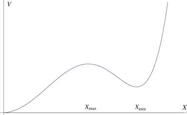
Figure 1: The sixth order of potential Eq. (2). On the false vacuum at $X=X_{min}$, the global $U(1)$ symmetry is spontaneously broken.

In the false vacuum, the global $U(1)$ symmetry is spontaneously broken. We simply assume that a global string is formed. Consider a static cylindrical solution of the field equation in the cylindrical coordinate, $(r,\theta,z)$. First we decompose $X$ into the radial and angular parts,

$$X=\eta R(r)e^{in\theta}\quad(n=1,2,3,\cdots).$$ (5)

Then the explicit form of the equation of $R(r)$ is obtained from Eq. (4)

$$\frac{\partial^{2}R}{\partial x^{2}}+\frac{1}{x}\frac{\partial R}{\partial x}-\frac{n^{2}}{x^{2}}R=(\delta+\zeta^{4})R+\zeta^{4}(3R^{5}-4R^{3}),$$ (6)

where $x=\epsilon r\eta$. We look for the solution where the scalar field in the interior of the string stays in the true vacuum, and that stays in the meta-stable vacuum at the exterior. That is, such a solution should satisfy $R=0$ at $x=0$ and $R\to R_{\rm min}$ at $x\to\infty$.

Here we emphasize that there can be a (meta)stable tube-like solution. Since the string core has lower energy density than that of its exterior, larger string radius seems to be favorable for the system, which predicts the roll-over process. However, there must be the domain wall between its core and exterior, whose energy becomes larger for larger string radius. As a result, there arises a (meta)stable tube-like solution, depending on the parameters. We will see it in more detail in the next section.

The static axial-symmetric solutions can be obtained by solving Eq. (6) with the successive over-relaxation method with the relaxation factor $\omega=1.0,0.5$ and $0.3$ for $n=1,2,3$, respectively. See the Appendix for details of our numerical schemes. Using the boundary conditions $R(r_{\rm b})=R_{\rm min}$ and $R(0)=0$, we find stable solutions. In Fig. 2, we plot the field configurations (left panel) and the potential energies (right panel) of the numerical solutions with $\epsilon=0.1,\zeta=4.0$ and $\delta=1.0$ for $n=1,2,3$. We confirmed that the field configurations are insensitive to the position of boundary, $r_{\rm b}$, as long as it is sufficiently far from the domain wall. At the region where the potential energy becomes a peak, there is a domain wall which is the surface of the tube/cylinder. It is found that the radius of the tube/cylinder depends on the winding number, $n$, and the higher-winding solution tends to be thicker. Moreover, the thickness of the domain wall is quite insensitive to the winding number.

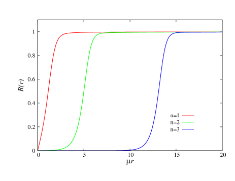
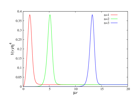
Figure 2: The radial field configuration $R(r)$ (left) and their potential energies (right) with $\epsilon=0.1$, $\zeta=4.0$, and $\delta=1.0$.

III Analytic estimations

III.1 A schematic illustration of stability of the tube-like string and bubble

In the previous section, we demonstrate numerical solutions for the static tube-like string. Before we consider the detailed estimation of their structure, we here give a rough approximation and clarify the stability of those solutions by using a simple thin-wall approximation. It is obvious that the stability of the tube-like string depends on the difference in the energy density of the true and false vacua

$${\tilde{\epsilon}}=V_{\rm false}-V_{\rm true}=V_{\rm min}\simeq\delta\mu^{2}\eta^{2}.$$ (7)

When ${\tilde{\epsilon}}=0$ $(\delta=0)$, the vacua inside and outside the string have the same energy. Then the tube-like string is stable because it is supported by the topological reason. On the other hand, when ${\tilde{\epsilon}}$ is large enough, the core energy density wins out and the string grows and expands. Thus, one expects that there exists a metastable tube-like string in an intermediate range for ${\tilde{\epsilon}}$. Let us clarify this by using the thin-wall approximation where the wall of the string is thin compared to the core and the exterior. The thin wall’s contribution to the energy density can be approximated by the constant surface energy, $\sigma$. Then, the tension of the string with radius $w$ is estimated by

$$E(w)=n^{2}C\log\frac{r_{c}}{w}+\sigma w-{\tilde{\epsilon}}w^{2},$$ (8)

where the first term is the contribution of the flux of the $U(1)$ global current with $r_{c}$ being a cutoff scale and $C\simeq 2\pi\eta^{2}$ being a constant of a mass dimension 2, the second term is of the wall and the last term is of the core of the tube-like string. Here we assume ${\tilde{\epsilon}},\sigma$, and $C$ are independent of $w$.

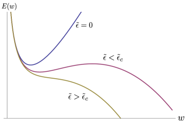
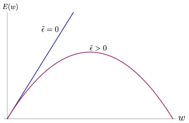
Figure 3: A string energy (left) and a bubble energy (right) as functions of the core radius $w$.

The dependence of the string energy on ${\tilde{\epsilon}}$ is shown in Fig. 3. When ${\tilde{\epsilon}}=0$, as we explained, there exists a local minimum, which implies that there exists a stable tube-like string. In the region $0<{\tilde{\epsilon}}<{\tilde{\epsilon}}_{c}$ with ${\tilde{\epsilon}}_{c}=\frac{\sigma^{2}}{8Cn^{2}}$, there exist a local minimum and a global maximum at

$$w_{\rm min}=\frac{\sigma-\sqrt{\sigma^{2}-8Cn^{2}{\tilde{\epsilon}}}}{4{\tilde{\epsilon}}},\quad w_{\rm max}=\frac{\sigma+\sqrt{\sigma^{2}-8Cn^{2}{\tilde{\epsilon}}}}{4{\tilde{\epsilon}}}.$$ (9)

In this case the tube-like strings exist but they are metastable. The tube-like string whose core radius is larger than $w_{\rm max}$ is unstable. When ${\tilde{\epsilon}}$ exceeds the critical value, ${\tilde{\epsilon}}>{\tilde{\epsilon}}_{c}$, there are no local minima at all. Namely, the string is unstable and the string core expands infinitely. In this paper the metastable strings are concerned. Although they are metastable as static configurations, they will become unstable in some dynamical processes such as string collision, annihilation and reconnections.

From Eq. (8) with $n$ being zero, the fate of the two-dimensional bubble can be also clarified. As shown in Fig. 3, the bubble never grows if ${\tilde{\epsilon}}=0$. Once the positive ${\tilde{\epsilon}}$ is turned on, the bubble becomes metastable. The critical radius of the bubble is $w_{c}=\frac{\sigma}{2{\tilde{\epsilon}}}$. The bubble lager than $w_{c}$ expands infinitely and the true vacua inside the core wins out. There are no metastable tube-like solutions.

The thin-wall approximation explained above is simple and gives an insight about the stability problem. Nevertheless, it is of only limited accuracy and we need a better analysis to get more quantitative results beyond the qualitative properties. To go beyond the thin-wall approximation, we will work out another analytical study in the next subsections.

III.2 Thickness of walls

Now let us go beyond the thin-wall approximation and consider the stability of the tube-like solution in more detail. From the numerical calculations of stable static solutions, we found that the tube-like solution is well characterized by the radius of cylinders, $w$, the winding number, and the thickness of the walls, $d$. Since the thickness of the wall is quite insensitive to other two parameters, it is possible to estimate $d$ from the variation of the total energy $E$ with respect to $d$, and it can be done by considering only the case of $n=1$.

We here simply approximate the solution with $n=1$ as the following piecewise linear function

$$R(r)\approx\begin{cases}\displaystyle\frac{r}{d}R_{\rm min}&r<d\\ R_{\rm min}&d<r\end{cases},$$ (10)

where we set $w=0$, see Fig. 2. Then, we approximate the volume integral of the potential energy and gradient energies as

$$E_{\rm potential} =\pi d^{2}(V_{\rm max}-V_{\rm min}),$$ (11)

$$E_{\rm grad,r} =\pi\eta^{2}R_{\rm min}^{2},$$ (12)

$$E_{\rm grad,\theta} =\pi\eta^{2}R_{\rm min}^{2}\left(1+2\log\frac{r_{c}}{d}\right).$$ (13)

The derivative of the summation of these energy components with respect to $d$ gives the desired value of $d$,

$$\frac{\partial E}{\partial d}=2\pi d(V_{\rm max}-V_{\rm min})-2\pi\eta^{2}\frac{R_{\rm min}^{2}}{d}=0\quad\Longrightarrow\quad d=\frac{\eta R_{\rm min}}{\sqrt{V_{\rm max}-V_{\rm min}}}=\frac{3}{2\eta\epsilon\zeta^{2}}\sqrt{\frac{c+2}{c^{3}}}.$$ (14)

III.3 Upper bound of winding number

We consider how the radius of the cylinder is determined and the upper limit of the winding number with which the static solution exists. As shown in Fig. 2, for $n\geq 2$, there are two parameters characterizing a cylinder, the radius $w$ and the thickness $d$ of the surface. However, as shown in the previous subsections, the latter one is not sensitive to the winding number and is determined from $V_{\rm max}-V_{\rm min}$. Hence we here focus on the radius $w$ of the cylinder while the width of the wall $d$ is assumed to be the same as one given in Eq. (14).

We simply approximate the solution and the potential as

$$R(r)\approx\begin{cases}0&\\ \displaystyle\frac{r-w}{d}R_{\rm min}&\\ R_{\rm min}&\end{cases},V(r)\approx\begin{cases}0&r<w\\ V_{\rm max}&w\leq r<w+d\\ V_{\rm min}&w+d<r\end{cases}.$$ (15)

The volume integral of the potential energy is approximated as

$$E_{\rm potential}=-V_{\rm min}\pi w^{2}+\pi d(2w+d)(V_{\rm max}-V_{\rm min}),$$ (16)

where we considered only the deviation from $V_{\rm min}$. On the other hand, that of the gradient energy can be divided into the radial and angular parts,

$$E_{\rm grad,r} =2\pi\eta^{2}\int_{0}^{\infty}\!R^{\prime}(r){}^{2}\,rdr=\pi\eta^{2}R_{\rm min}^{2}\left(2\frac{w}{d}+1\right),$$ (17)

$$E_{\rm grad,\theta} =2\pi n^{2}\eta^{2}\int_{0}^{\infty}\!\frac{R^{2}}{r^{2}}\,rdr=2\pi n^{2}\eta^{2}R_{\rm min}^{2}\left[\frac{1}{2}-\frac{w}{d}+\frac{w^{2}}{d^{2}}\log\left(1+\frac{d}{w}\right)+\log\left(\frac{r_{c}}{w+d}\right)\right],$$ (18)

where $r_{c}$ is the cut-off length, $r_{c}\to\infty$, and it should be properly regularized. Then the total energy becomes

$$E=E_{\rm potential}+E_{{\rm grad},r}+E_{{\rm grad},\theta}.$$ (19)

Let us look for the values of $w$ to minimize the total energy. One can easily see that there is no global minimum of $E$ since the term proportional to $-w^{2}$ in Eq. (16) implies that $E\to-\infty$ for $w\to\infty$. Instead, we investigate whether there is a local minimum in the region, $w>0$. The derivative of $E$ with respect to $w$ is calculated as

$$\frac{dE}{dw} =\frac{2\pi\eta^{2}R_{\rm min}^{2}}{d}G(w),$$ (20)

$$G(w) \equiv-2p\frac{w}{d}+2+2n^{2}\left[-1+\frac{w}{d}\log\left(1+\frac{d}{w}\right)\right],$$

where

$$p\equiv\frac{d^{2}V_{\rm min}}{2\eta^{2}R_{\rm min}^{2}}=\frac{V_{\rm min}}{2(V_{\rm max}-V_{\rm min})}.$$ (21)

What we have to do is to find $w$ to satisfy $G(w)=0$ for $w>0$. We plot $E(w)$ and $G(w)$ with specific values of $\epsilon,\zeta$ and $\delta$ in Fig. 4. From the right panel of this figure, it is found that there are two zero-points for $n\leq 6$, and the smaller one is the desired value of $w$, at which $E$ is locally minimized, and the other zero-point gives the local maximum of $E$ (see the corresponding lines in the left panel). Note that the local minimum of $n=1$ is $w=0$, which is consistent with the numerical solution in Fig. 2.

In order for these zero-points to exist, the local maximum of $G(w)$ should be positive. Actually, $G(w)$ for $n=7$ is always negative, and in the left panel of Fig. 4 the line for $E(w)$ with $n=7$ has no local minimum, which indicates the cylinder solution with $n=7$ is unstable. To proceed this calculation, we assume $d/w\ll 1$ to expand the logarithm function. Then we find that $G(w)$ has a local maximum,

$$G(w_{c})\simeq 2-2n\sqrt{2p},\quad w_{c}\simeq\frac{nd}{\sqrt{2p}}.$$ (22)

Therefore the condition on the winding number required for the local minimum of $E$ is

$$G(w_{c})>0\quad\Longrightarrow\quad n<\frac{1}{\sqrt{2p}}=\sqrt{\frac{V_{\rm max}-V_{\rm min}}{V_{\rm min}}}.$$ (23)

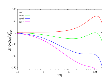
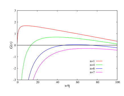
Figure 4: An example of $E(w)/(2\pi\eta^{2}R_{\rm min}^{2})$ (left) and $G(w)$ (right) with specific values of $\epsilon=0.1,\zeta=4.0,$ and $\delta=1.0$.

III.4 Instability of spherical bubble and critical volume

In subsection III.1 we have seen that the two-dimensional bubble is unstable and it shrinks (expands) when its radius is smaller (larger) than the critical value. Here, we study the spherically symmetric configuration (three-dimensional bubble) of the scalar field separated by the domain wall. It is also expected to be always unstable. After two cylinders collide with each other, there appears a spherical object at the impact point. To study the instability of such an object, we consider the following ansatz in the spherical coordinate,

$$R(r)\approx\begin{cases}0&\\ \displaystyle\frac{r}{d}R_{\rm min}&\\ R_{\rm min}&\end{cases},V(r)\approx\begin{cases}0&r<w\\ V_{\rm max}&w<r<w+d\\ V_{\rm min}&d<r\end{cases},$$ (24)

with assuming that $d$ is given by Eq. (14). We simply assume that the field is homogeneous in the azimuthal and the polar directions. The potential and radial gradient energy are approximated as

$$E_{\rm potential} =-\frac{4}{3}\pi w^{3}V_{\rm min}+\frac{4}{3}\pi\{(w+d)^{3}-w^{3}\}(V_{\rm max}-V_{\rm min}),$$ (25)

$$E_{\rm grad,r} =\frac{4}{3}\pi\left(\frac{R_{\rm min}}{d}\right)^{2}\{(w+d)^{3}-w^{3}\}\eta^{2},$$ (26)

and thus the total energy becomes

$$E(w)=\frac{4}{3}\pi\left[-w^{3}V_{\rm min}+2\{(w+d)^{3}-w^{3}\}(V_{\rm max}-V_{\rm min})\right],$$ (27)

where we used Eq. (14) to eliminate $R_{\rm min}$. The function $E(w)$ has the only peak at $w=w_{c}$ in $w>0$, and the critical radius $w_{c}$ is given by solving $dE/dw=0$,

$$w_{c}=\frac{1+\sqrt{1+p}}{p}d,$$ (28)

where $p$ is defined in Eq. (21). For $w<w_{c}$ the radius of the sphere starts to shrink since $dE/dw>0$. On the other hand, for $w>w_{c}$ the radius goes to the positive infinity since $dE/dw<0$. That is, if the volume of the spherical object is larger than the critical volume $4\pi w_{c}^{3}/3$, this grows infinitely.

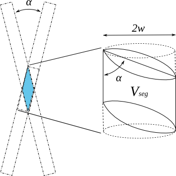
Figure 5: The volume colliding with another cylinder.

Now we give an analytical estimate of the (in)stability of the colliding cylinders. Let us consider the situation that two cylinders collide with the collision angle $\alpha$ as shown in Fig. 5. Assuming that a spherical object is produced via the fusion of two cylinders after collision and its volume is equal to the total volume of the two colliding segments of cylinders, $2V_{\rm seg}$, the initial volume of the spherical object is calculated as

$$V_{\rm total}=2V_{\rm seg}=\frac{4\pi w^{3}}{\sin\alpha}.$$ (29)

Then the condition for the sphere to grow infinitely is given by

$$\frac{4\pi}{3}w_{c}^{3}<V_{\rm total}\;\;\Longrightarrow\;\;\sin\alpha<3\left(\frac{w}{w_{c}}\right)^{3},$$ (30)

where $w$ is obtained by solving $G(w)=0$ in Eq. (20), and hence assuming $d/w\ll 1$, this is calculated as

$$w=\frac{1-\sqrt{1-2n^{2}p}}{2p}d.$$ (31)

As a result, we obtain the upper limit of the collision angle so that the spherical object created at the impact point can grow infinitely,

$$\sin\alpha<\frac{3}{8}\left(\frac{1-\sqrt{1-2n^{2}p}}{1+\sqrt{1+p}}\right)^{3}.$$ (32)

For example, $\epsilon=0.1,\zeta=4.0$ and $\delta=1.0$ give the upper limit, $\alpha<7.78\times 10^{-6}$, for $n=2$, and $\alpha<2.50\times 10^{-2}$ for $n=6$.

IV Simulation setup

We explore the (in)stability of collision processes of two meta-stable strings. The individual string is given by the axial-symmetric solution which is numerically obtained by solving Eq. (4) without the time-derivative term, corresponding to Eq. (6). This procedure is nothing but the one-dimensional boundary value problem, and is carried out with the Gauss-Seidel method. Each of the resultant strings is put on the x-z surface parallel to each other separated a bit. The strings are Lorentz-boosted to collide with each other at an angle with $\alpha$ measured on the x-z surface including the origin (to be the impact point when colliding). The free model parameters are $\epsilon$ and $\zeta$, which control the strength of the self-coupling and the energy scale of the phase transition, respectively. The fiducial parameters are listed in Table 1. Note that we choose $\zeta=2.2$ for numerical simulations, while $\zeta=4.0$ has been used so far, to enhance the instability.

The initial separation between the strings is fixed to be $20\eta^{-1}$, while the radius of the string is about $5\eta^{-1}$ for the fiducial choice of parameters. According to Ref. Vilenkin , the superposition of the two strings is given by

$$X=\frac{X_{1}X_{2}}{\eta R_{\rm min}},$$ (33)

where the denominator is determined by the dimension analysis and the fact that $|X|\to\eta R_{\rm min}$ far away from two strings.

Then we solve Eq. (4) in the three-dimensional cartesian coordinate with the Neumann conditions on the boundaries, $\partial X/\partial n^{i}|_{\rm boundary}=0$, where $n^{i}$ is the normal vector to each boundary. We use the Leap-frog method for the time domain and approximate the spatial derivatives by the 2nd-order central finite difference. The simulations are stopped at $t=L/2$, when the information at the impact point arrives at the nearest boundary of the computational domain.

model parameters
$\epsilon$	0.1
$\zeta$	2.2
$\delta$	1.0
$n_{1}$	1
$n_{2}$	1

simulation parameters
grid size	$N$	$480^{3}$
box size	$L$	240$\eta^{-1}$
time interval	$\Delta t$	$0.2\eta^{-1}$
total steps	$N_{\rm s}$	600
simulation time	$t_{f}$	$120\eta^{-1}$

Table 1: The fiducial parameters.

V Results

Through the numerical simulations, we find that the collision processes end up with either simply reconnecting and going away from each other, or creating unstable objects with a higher winding number at the impact point. Figs. 6-11 show the snapshots of the computational domain during simulations, the leftmost panel is at the initial time $t=0$, and the rightmost one at the final time $t=t_{f}$. The surfaces in them represent $X=X_{\rm max}$ given in Eq. (3), and hence in the interior of them the field $X$ lies in the true vacuum. The first four figures, Figs. 6-9, are the cases of parallel strings with relatively small $\alpha$, and the remaining ones, Figs. 10 and 11, are those of anti-parallel strings with $\alpha\sim\pi$. Moreover, we plot the field configurations and those phases on the surface at $z=L/2$ and $t=t_{f}$ in Figs. 12 and 13. In the unstable cases, P1, P3, P4 and A1, we find that the true vacuum homogeneously spreads over the interior of the bubbles. As for the phases, one can observe that the winding number is conserved. For the parallel pairs, one can find that the total winding number is $n=1+1=2$ (two sets of blue$\to$green$\to$red$\to$blue), if one follows the trajectory around the bubble. In the interior, there seems to be a large number of points around which the phase is rotated, although the winding vanishes if one follows the trajectory around the impact point. On the other hand, for the anti-parallel pairs, the total winding number around the bubble becomes $n=1-1=0$ (green$\to$blue$\to$green$\to$red$\to$blue$\to$red$\to$green.)

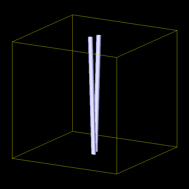
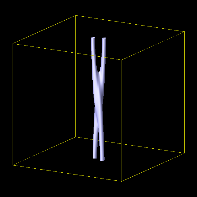
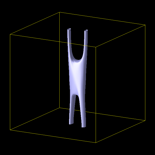
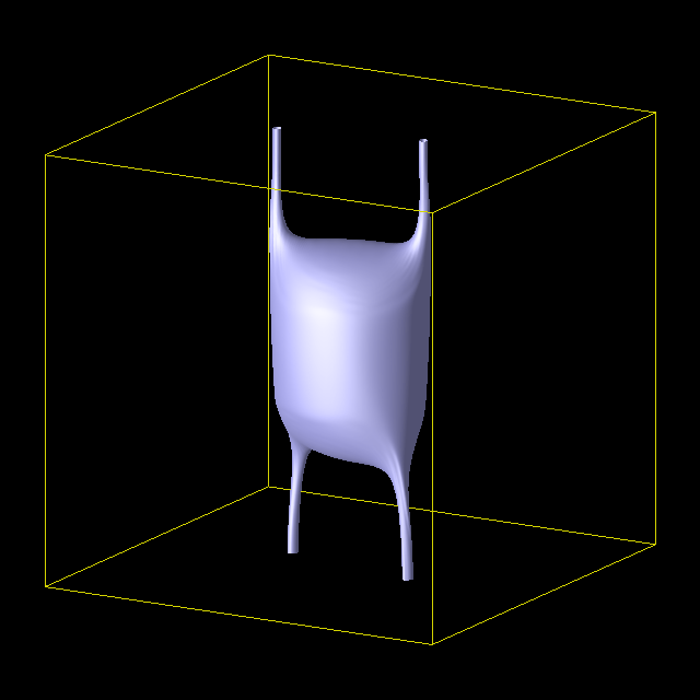
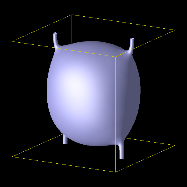
Figure 6: [P1] Failed reconnection of parallel string pair with $(v,\alpha)=(0.82c,0.02\pi)$. See animation for full animations.

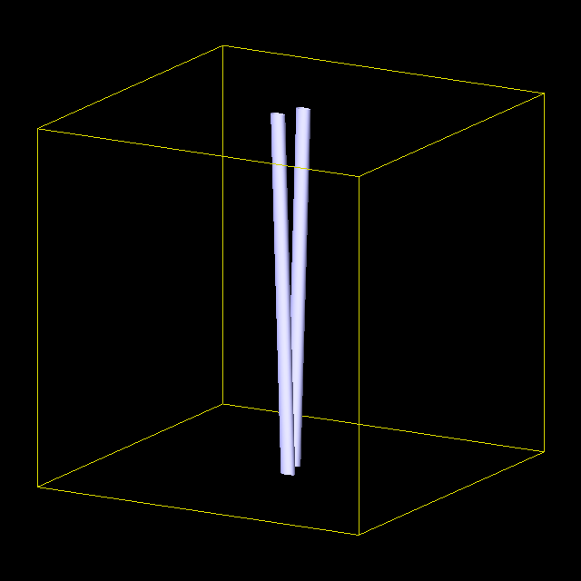
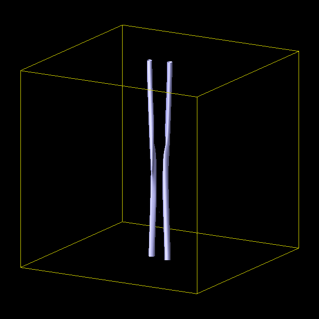
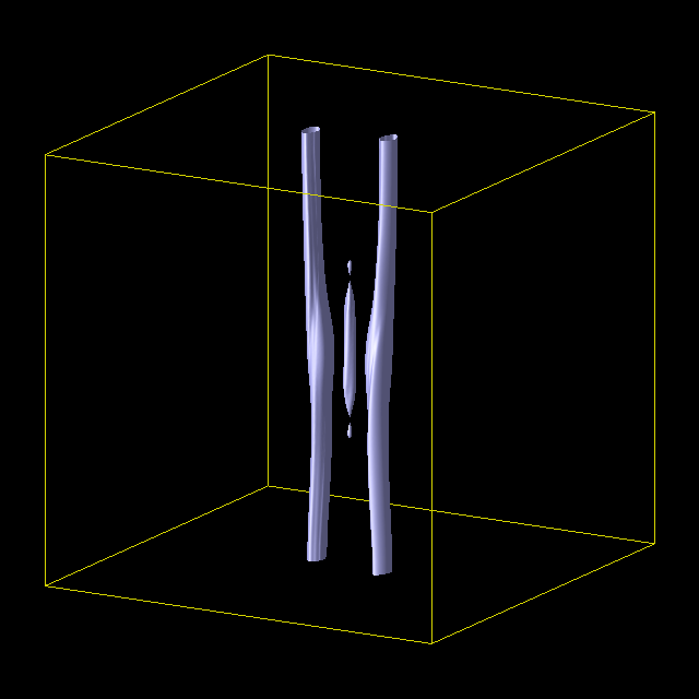
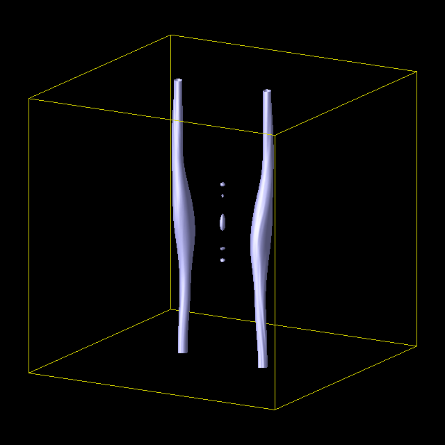
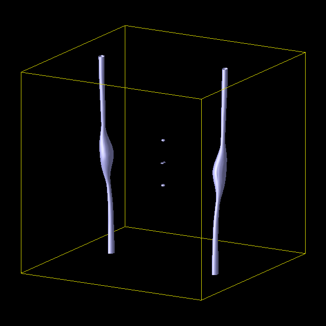
Figure 7: [P2] Successful reconnection of parallel string pair with $(v,\alpha)=(0.90c,0.02\pi)$. See animation for full animations.

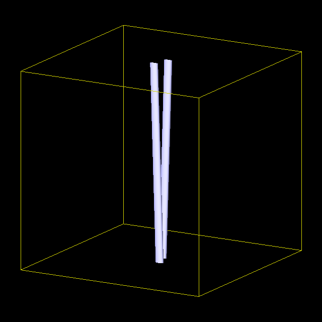
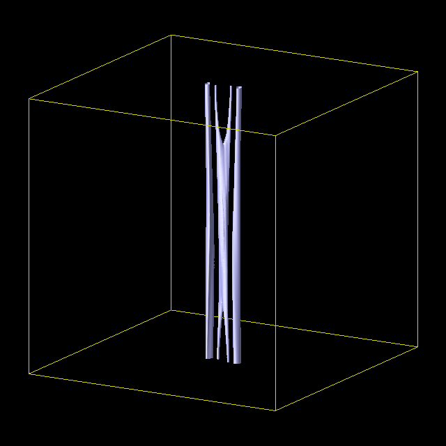
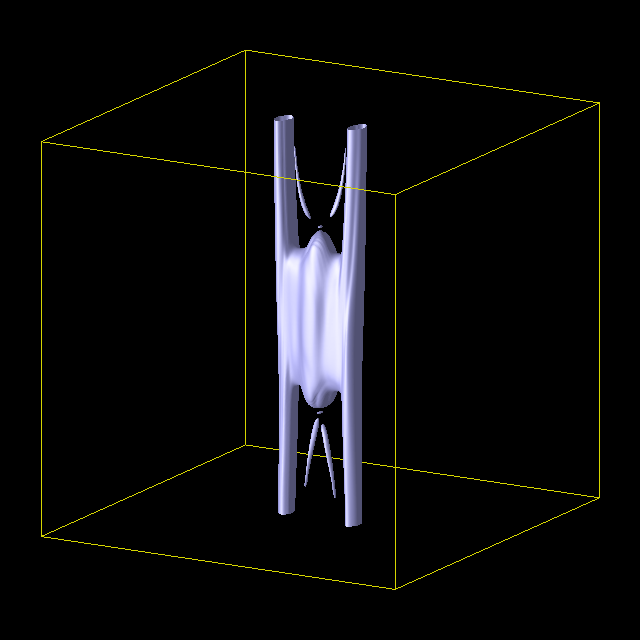
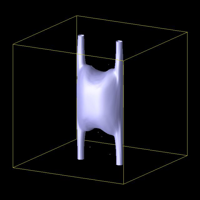
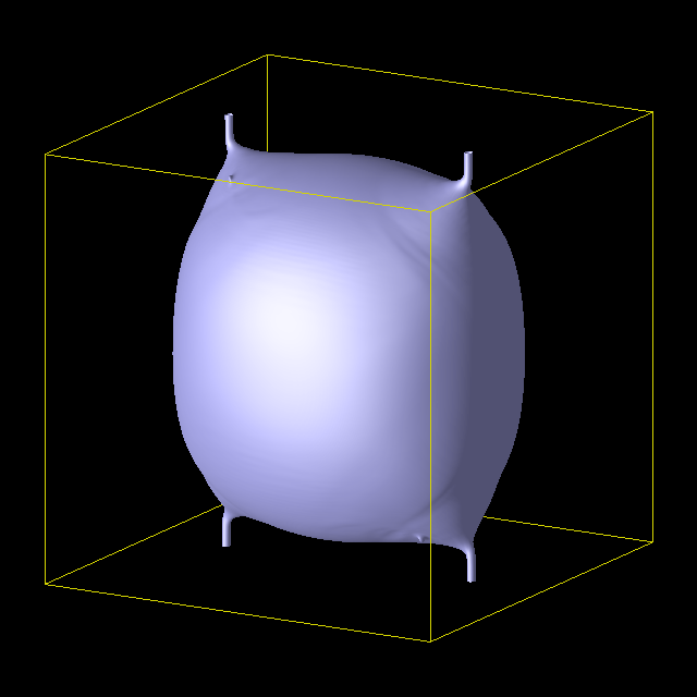
Figure 8: [P3] Failed reconnection of parallel string pair with $(v,\alpha)=(0.94c,0.02\pi)$. See animation for full animations.

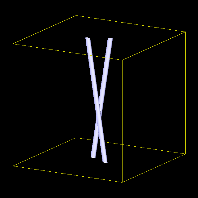
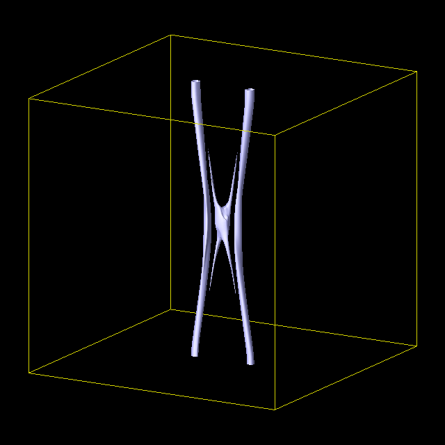
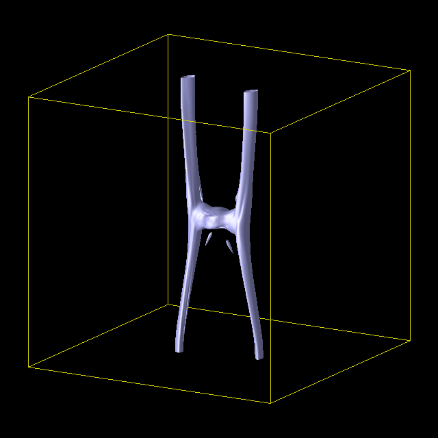
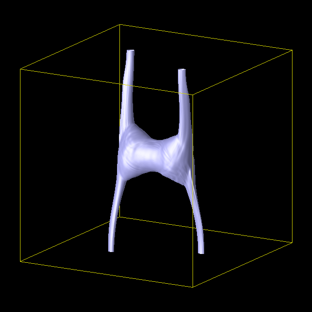
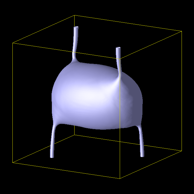
Figure 9: [P4] Failed reconnection of parallel string pair with $(v,\alpha)=(0.95c,0.10\pi)$. See animation for full animations.

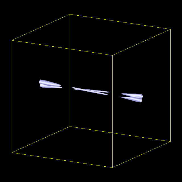
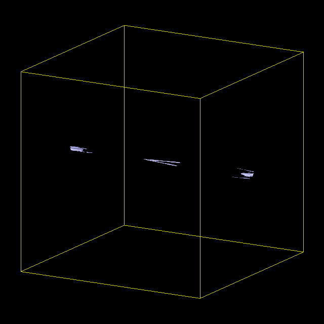
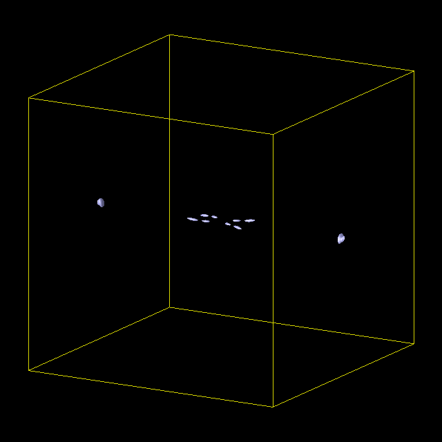
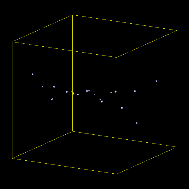
Figure 10: [A1] Anti-parallel string pair with $(v,\alpha)=(0.62c,0.94\pi)$. Most of segments are annihilated. See animation for full animations.

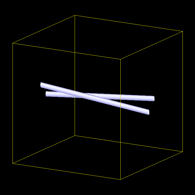
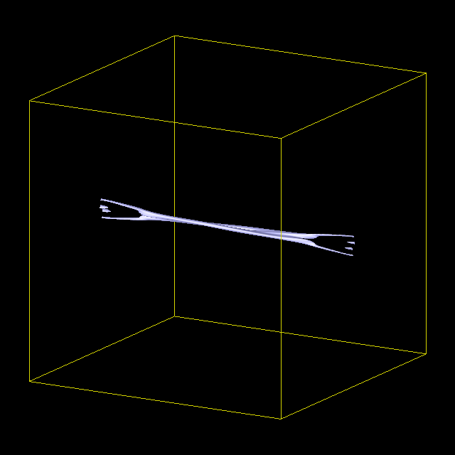
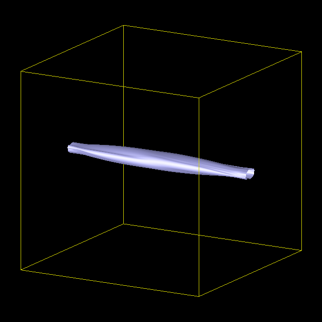
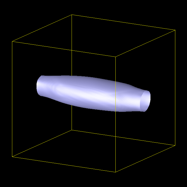
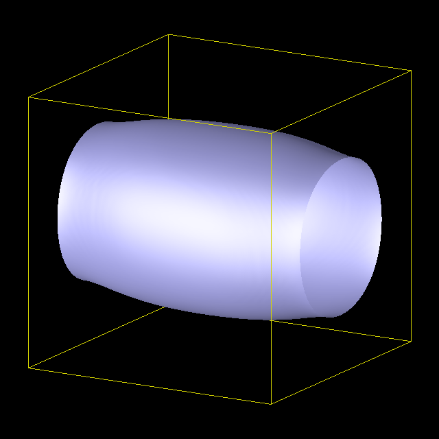
Figure 11: [A2] Anti-parallel string pair with $(v,\alpha)=(0.90c,0.94\pi)$. After collision, the true vacuum region is created around the impact point, and it starts to grow exponentially. See animation for full animations.

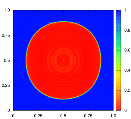
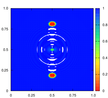
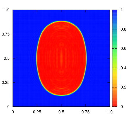
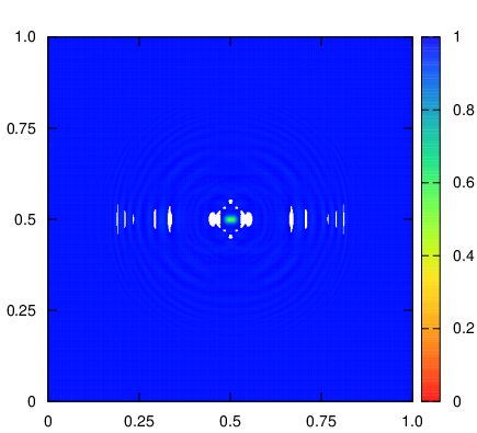
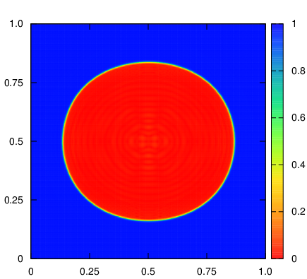
Figure 12: The field configurations of [P1]-[P4] on $z=L/2$ (upper panels), and those of [A1], [A2] on $y=L/2$(lower panels) at $t=t_{f}$. The colour contour represents $|X|/R_{\rm min}$. The white colour indicates the overshoot, $|X|>R_{\rm min}$.

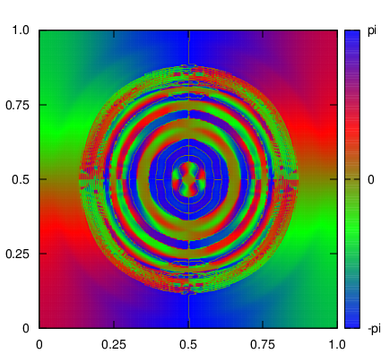
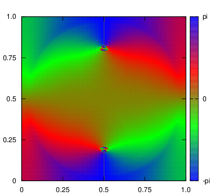
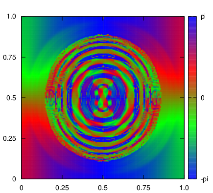
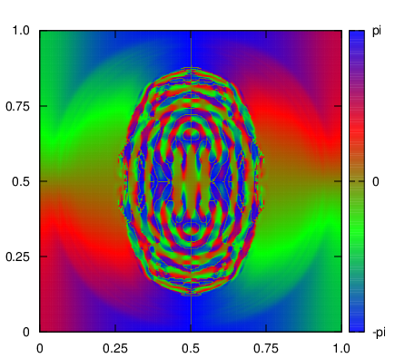
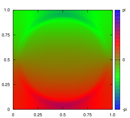
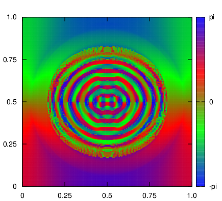
Figure 13: The phases of [P1]-[P4] on $z=L/2$ (upper panels), and those of [A1], [A2] on $y=L/2$ (lower panels) at $t=t_{f}$.

The (in)stability of a resultant string after collision depends on the velocity of two cylinders, $v$, and the collision angle between them, $\alpha$. We surveyed the parameter space $(\alpha,v)$ to check the stability. Fig. 14 shows the stability of parallel string pairs, and Fig.15 that of anti-parallel pairs where $\alpha$ is close to $\pi$. In order to systematically judge the resultant stability, we calculate two quantities and set a criterion for each. One is the growth rate of the volume of the true vacuum region during simulation,

$$\kappa_{1}=\frac{\mathcal{V}_{\rm true}(t=t_{f})}{\mathcal{V}_{\rm true}(t=0)},$$ (34)

and the other is the ratio of time when the true vacuum region grows to the total simulation time,

$$\kappa_{2}=\frac{t_{\rm grow}}{t_{f}},\qquad t_{\rm grow}=\Delta t\times\sharp\left\{t_{m}\Bigg{|}\left.\frac{d\mathcal{V}_{\rm true}}{dt}\right|_{t=t_{m}}>0\right\},$$ (35)

where $\sharp$ denotes the number of elements, $\Delta t$ is the time interval, and $t_{m}$ represents the discrete time, $t_{m}=m\Delta t$. If and only if both $\kappa_{1}>\kappa_{1c}$ and $\kappa_{2}>\kappa_{2c}$ are satisfied, we decide that the resultant strings become unstable, and thus the true vacuum region grows exponentially. We set $\kappa_{1c}=10$ and $\kappa_{2c}=0.8$. The second quantity, $\kappa_{2}$, measures how monotonic the instability grows. After all, however, most of (in)stabilities can be determined by the first one, $\kappa_{1}$.

In Figs. 14 and 15, we plot red filled circles for unstable pairs, and green crosses for stable pairs. We find that the slow collision with small $\alpha$ results in the failure of the reconnection and thus being unstable, and quite high-speed collision can also make the system unstable in both cases with small (parallel pair) and large $\alpha$ (anti-parallel pair). In these figures, we also plot black circles labelled as P1,2,3,4 and A1,2. The corresponding figures were already shown in Figs. 6-11, which are the typical examples of several regions leading to stable and unstable processes in Figs. 14 and 15.

We explain in detail the mechanism of stable/unstable reconnection processes using Figs. 6-11. Firstly, for the parallel pairs, our findings are followings.

• (relatively slow collision) : Two strings merge at the instance of impact and cannot be separated from each other because of a small collision velocity. Then the effective volume of the merged strings around the impact point exceeds the critical volume mentioned in Sec.III, thus making the system unstable.

• (moderate-speed collision) : Two strings can safely reconnect with each other. As shown in the middle panel and its right neighbour, a small bubble is created at the impact points of the strings. However, since the reconnected strings rapidly go away from the bubble and the volume of the bubble is relatively small, the bubble finally shrinks. As a result, the system becomes stable.

• (high-speed collision) : Because of the large collision velocity, the kinetic energy induced to the bubble at the impact point is large enough to inflate the bubble until its volume exceeds the critical one. Finally the system becomes unstable.

• (large angle high-speed collision ) : Since the collision angle is large, the initial impact of strings cannot create a larger bubble at the impact point than the critical volume. However, kinetic energy induced to the bubble is too large, and then the bubble can rapidly expand (the third panel). At the same time, the reconnected strings also rapidly go away from the impact point. As a result, the bubble is about to break up (forth panel). Finally, the expansion rate of the bubble overcomes (last panel).

As for the anti-parallel pairs, they annihilate with each other in most of cases owing to the cancellation of their winding numbers [A1]. It is, however, surprising that the high-speed collision makes the system unstable. Actually, after the collision, a bubble with no windings is excited at the impact point, and it grows exponentially.

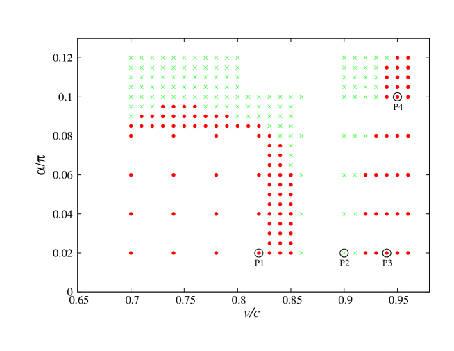
Figure 14: The parameter region for stable/unstable collision process for string-string collision.

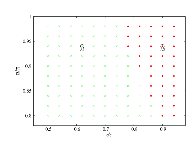
Figure 15: The parameter region for stable/unstable collision process for string-antistring collision.

VI Conclusion

We have studied the dynamical (in)stabilities of metastable strings after their collision in the model where the potential of a complex scalar field has a false vacuum state corresponding to a SUSY breaking vacuum in realistic SUSY models.

Before performing numerical simulations for the collision, we analytically investigated in a simplified model the thickness of the domain wall constituting the surface of strings, and the existence of static solutions with large winding numbers from the viewpoint of energetics. As a result, we found that the thickness of wall is determined from the shape of given potential, being independent of the winding number of strings, and there exists the upper bound of winding number for the stable solutions. Furthermore, in the same manner, we investigated the collision process of two metastable strings with some approximations neglecting the details of dynamics. Then we found that there is the critical volume of the true vacuum region in a string as indicated in Eq. (28) so that the instability grows, and thus in some cases with a small collision angle, the reconnection is failed.

After that, we performed three-dimensional field-theoretic simulations of two colliding metastable strings. The initial condition is given as the superposition of two Lorentz-boosted strings obtained in another numerical way. We surveyed the (in)stabilities of the collision processes on the parameter space $(v,\alpha)$, where $v$ is the velocity of strings and $\alpha$ is the collision angle.

Consequently, we found that the instability cannot always be observed for the string-string pairs. We fixed the winding number of strings as $n=1$ and tuned the parameters controlling the shape of potential, $\epsilon,\zeta$ and $\delta$, so that the static solution with $n=2$ does not exist. Nevertheless the strings with most of combinations $(v,\alpha)$ lead to successful reconnection, or, in other words, the parameter region in the $(v,\alpha)$ space where the instability grows is highly restricted.

We briefly explain the unstable cases. For small $\alpha$, we confirmed that the reconnection is failed owing to the rapid expansion of the overlap region just after the collision, shown in Fig. 6 [P1] and Fig. 8 [P3], as discussed in the static analysis mentioned above. In addition to this case, we found that the kinetic energy injected into the impact point can leads to failure reconnection. In fact, although the strings with a large velocity seem to succeed in reconnecting safely, the whole system becomes eventually unstable owing to the rapid growth of a true vacuum bubble created at the impact point after the collision, as shown in Fig. 8 [P3] and Fig. 9 [P4]. Surprisingly, this is also the case for the anti-parallel pair, as shown in Fig. 11 [A2], although one would envisage that they can pair-annihilate. This result would be explained by the shorter time scale of the expansion of the zero-winding bubble created at the impact point than that of pair-annihilation.

At first, we had a naive expectation such that the instability would grow because of the temporal formation of unstable $n=2$ strings at the moment of impact, and the anti-parallel pairs always annihilate after collision. Our numerical studies, however, clarified that this is not true story. Instead of the winding number iteself, it is confirmed that the volume of true vacuum at the impact point and the collision veclocity are responsible for the (in)stability of the colliding strings. Particularly, it should be stressed that the numerical studies presented here are crucial to find the latter fact, dependence on the velocity or kinetic energy of strings.

Our numerical study has shown the relatively complicated parameter dependence on the stability of tube-like strings against collisions, and will help to constrain the viable parameter space on concrete SUSY breaking models with spontaneous $U(1)_{R}$ symmetry breaking and also their cosmological history.

Appendix A numerical schemes

To find the static configuration of an axially symmetric metatable string, we solve Eq. (6) with the succesive over-relaxation method.

First of all, we discretise the coordinate such as $x_{j}=j\Delta x$ for $j=0,1,\ldots,N$, and represent the discretised $R(x)$ as a vector $R_{j}\equiv R(x_{j})$. The spatial derivatives in the left-hand side of Eq. (6) is replaced by the corresponding 2nd-order finite differences,

$$\left.\frac{d^{2}R}{dx^{2}}\right|_{x=x_{j}}\approx\frac{R_{j+1}-2R_{j}+R_{j-1}}{\Delta x^{2}},\qquad\left.\frac{dR}{dx}\right|_{x=x_{j}}\approx\frac{R_{j+1}-R_{j-1}}{2\Delta x}.$$ (36)

We denote the other terms depending on $R(x)$ in Eq. (6) by $S[R(x)]$ and those evaluated at $x=x_{j}$ by $S_{j}[R]\equiv S[R(x_{j})]$. Then the equation to be solved becomes

$$\frac{R_{j+1}-2R_{j}+R_{j-1}}{\Delta x^{2}}+\frac{R_{j+1}-R_{j-1}}{2x_{j}\Delta x}=S_{j}[R].$$ (37)

Solving this equations with respect to $R_{j}$ in the first term, we find trial values of $R_{j}$ denoted by $R_{j}^{*}$,

$$R_{j}^{*}=\frac{R_{j+1}+R_{j-1}}{2}-\frac{\Delta x^{2}}{2}\left(S_{j}[R]-\frac{R_{j+1}-R_{j-1}}{2x_{j}\Delta x}\right).$$ (38)

Notice that $R_{j}$ in $S_{j}[R]$ is not $R^{*}_{j}$. On each stage of iterations, we update $R_{j}$ so that

$$R_{j}^{(n+1)}=\omega R_{j}^{*}+(1-\omega)R_{j}^{(n)}.$$ (39)

This scheme with $\omega=1$ is equivalent to the Gauss-Seidel method. When we solve Eq. (6) for $\zeta=4.0$ in Sec. II, we set $\omega=1,0.5$ and $0.3$ for $n=1,2,3$, respectively. For $\zeta=2.2$ in Sec. IV, we set $\omega=1$.

References

- (1) A. Vilenkin and E.P.S.Shellard, Cambridge University Press, 1994.
- (2) K. A. Intriligator and N. Seiberg, Class. Quant. Grav. 24, S741 (2007) [hep-ph/0702069].
- (3) R. Kitano, H. Ooguri and Y. Ookouchi, Ann. Rev. Nucl. Part. Sci. 60, 491 (2010) [arXiv:1001.4535 [hep-th]].
- (4) P. J. Steinhardt, Nucl. Phys. B 190, 583 (1981); Phys. Rev. D 24, 842 (1981).
- (5) Y. Hosotani, Phys. Rev. D 27, 789 (1983).
- (6) U. A. Yajnik, Phys. Rev. D 34, 1237 (1986).
- (7) M. Eto, Y. Hamada, K. Kamada, T. Kobayashi, K. Ohashi and Y. Ookouchi, arXiv:1211.7237 [hep-th].
- (8) K. Kamada, T. Kobayashi, K. Ohashi and Y. Ookouchi, arXiv:1303.2740 [hep-ph].
- (9) http://www2.yukawa.kyoto-u.ac.jp/~hiramatz/research/metastable-strings/