Spectra of absolute instruments
from the WKB approximation

Abstract

We calculate frequency spectra of absolute optical instruments using the WKB approximation. The resulting eigenfrequencies approximate the actual values very accurately, in some cases they even give the exact values. Our calculations confirm results obtained previously by a completely different method. In particular, the eigenfrequencies of absolute instruments form tight groups that are almost equidistantly spaced. We demonstrate our method and its results on several examples.

1 Introduction

Absolute optical instrument (AI) is a device that provides a perfectly sharp image of all points in some spatial region [1]. The simplest AI is a plane mirror that gives a virtual image of a whole half-space. Another, beautiful example of an AI is Maxwell’s fish eye, discovered by J. C. Maxwell in 1854 [2], that images sharply the whole space, and all rays form circles. In recent years absolute instruments attracted an increased interest which has led to proposing new devices of various types, e.g. AIs that perform imaging of the whole space, of optically homogeneous regions [3, 4], or provide magnified images [5]. A general method has been proposed in [4] for designing spherically symmetric AIs. This research was based on geometrical optics.

Recently AIs attracted attention also from the point of view of wave optics. It was shown both theoretically [6] and experimentally [7, 8] that these devices can provide subwavelength resolution, although this claim has raised controversy [9, 10, 11] and it is still not clear to what extent such a super-resolution can be used practically [12]. A different question was addressed in  [13], namely what are the general characteristics of the spectrum of eigenfrequencies of AIs. It was shown that the spectrum consists of tight groups of levels with almost equidistant spacing between them. This finding was based on an analysis of a light pulse propagating in the AI and on the assumption that a short pulse emitted at some point can be absorbed at the image point during a short time as well. Numerically calculated spectra of various AI confirmed this theoretical result very well.

In this paper, we investigate the spectra of absolute instruments by a completely different method. Employing the WKB approximation with the Langer modification and using one of the general properties of AIs, we confirm in a different way the previously known results about their spectrum [13]. Our method has two advantages compared to the previous one: it enables to calculate not just the spacing of the level groups but also their offset, and it allows to treat the situations where a mirror is used in the device. We verify our results by comparing the calculated spectra with numerical values for several examples of AIs.

The paper is organised as follows. In Sec. 2 we recall absolute instruments and discuss some of their properties. In Sec. 3 we employ the WKB method for calculating the spectra of radially symmetric media and in Sec. 4 we illustrate the results on particular examples of AIs. In Sec. 5 we analyse the situation in AIs that contain mirrors, and we conclude in Sec. 6.

2 Absolute optical instruments

In this section we recall some properties of absolute instruments from the point of view of geometrical optics, which will be useful for the subsequent calculations. We will consider radially symmetric AIs with the refractive index distribution $n(r)$. In addition, we will focus on a specific class of absolute instruments, namely AIs of the first type [4]. AI of the first type is a device with the property that every point A from its whole volume has a full image at some point B, which means that all rays emerging from A reach B. Since the role of the points A and B can be interchanged, it is clear that any ray emerging from the point A returns back to this point again, so A is an image of itself. In some AIs, it is the only image, in other ones there may be more images.

The AI can be either three- or two-dimensional. In the latter case we consider a 2D propagation of rays in a 2D refractive index profile. Due to the radial symmetry of the device, the following quantity analogous to the mechanical angular momentum is conserved [1]:

$${L}=rn(r)\sin\alpha\,,$$ (1)

where $\alpha$ is the angle between the tangent to the particle trajectory and the radius vector. In 3D, another consequence of the radial symmetry of the device is that each ray lies in a plane containing the centre of symmetry of the device O, so the ray trajectory can be described in polar coordinates $(r,\varphi)$ both in the 2D and 3D cases. For nonzero ${L}$, the polar angle $\varphi$ increases (or decreases) monotonically while $r$ oscillates between the turning points $r_{-}$ and $r_{+}$, $r_{-}\leq r_{+}$. We will assume that for each possible value of $L$, there are just two turning points that coalesce when $L$ reaches its largest possible value $L_{0}$.

In order to ensure that any ray emerging from a point A eventually returns there, the change of the polar angle $\Delta\varphi$ corresponding to $r$ changing from $r_{-}$ to $r_{+}$ must be a rational multiple of $2\pi$, so we can write $\Delta\varphi=\pi/\mu$, $\mu\in{\mathbb{Q}}$. We will assume in this paper that the value of $\mu$ is the same for all possible angular momenta $L$, which is the most usual case. With respect to this assumption and since any point is an image of itself, the optical path $S_{\rm AA}=\int n\,{\rm d}l$ from A back to A is equal for all rays [1]. At the same time, the ray from A back to A consists of an integer number of segments on each of which $r$ changes from $r_{-}$ to $r_{+}$ or back. Therefore also the optical path $S$ between two turning points has to be equal for all rays, i.e., it is independent of the angular momentum $L$. This optical path can in general be expresses as

$$S({L})=\int_{r_{-}}^{r_{+}}\frac{n\,{\rm d}r}{\cos\alpha}=\int_{r_{-}}^{r_{+}}\frac{n\,{\rm d}r}{\sqrt{1-({L}/nr)^{2}}}\,,$$ (2)

where we have used Eq. (1) and written the dependence on $L$ explicitly. The fact that for absolute instruments $S$ is independent of $L$ is of a key importance for calculation of the spectra with the WKB method, as we will see in the following section.

As the last thing we will express the optical path between the turning points in a different way. When $L$ increases, the turning points $r_{\pm}$ approach each other and finally meet at the point $r_{0}$, the radius of the circular ray, for the maximum possible value of angular momentum $L=L_{0}$. The corresponding optical path $S$ is then equal to the geometrical path $\Delta\varphi r_{0}=\pi r_{0}/\mu$ multiplied by the refractive index $n(r_{0})$, i.e.,

$$S=\frac{\pi r_{0}n(r_{0})}{\mu}\,.$$ (3)

3 WKB calculation of spectra of AIs

For simplicity we will consider a monochromatic scalar wave in the AI that can be described by the Helmholtz equation

$$\Delta\psi+k^{2}n(r)^{2}\psi=0\,.$$ (4)

If the speed of light is set to unity, $k$ is at the same time equal to the frequency $\omega$ of the wave. Separating the radial and angular parts in terms of $\psi(r,\theta,\varphi)=R(r)Y_{lm}(\theta,\varphi)$ (in 3D) or $\psi(r,\varphi)=R(r){\rm e}^{{\rm i}m\varphi}$ (in 2D) and making the substitution $R(r)=r^{-1}w(r)$ (in 3D) or $R(r)=r^{-1/2}w(r)$ (in 2D), we get the equation for $w(r)$ in the form

$$w^{\prime\prime}+\left[-\frac{l(l+1)}{r^{2}}+k^{2}n^{2}\right]w=0\quad\mbox{(3D)},\qquad w^{\prime\prime}+\left[-\frac{m^{2}-1/4}{r^{2}}+k^{2}n^{2}\right]w=0\quad\mbox{(2D)}\,,$$ (5)

where the prime denotes a derivative with respect to $r$.

The equations (5) are analogous to the radial part of the Schrödinger equation obtained when solving a quantum-mechanical motion in a central potential. As was shown by Langer [14], however, a direct application of the WKB method to that equation leads to problems due to the centrifugal potential and termination of the $r$-axis at $r=0$, and yields wrong results for the energy spectrum of the system. A careful analysis shows that the problem can be eliminated by the substitution $l(l+1)\to(l+1/2)^{2}$ (or $m^{2}-1/4\to m^{2}$ in 2D) — the so-called Langer modification, see [14, 15] or § 49 of [16]. Then the WKB method can be applied to the resulting equation directly and gives correct results. Exactly the same argument applies also in our case, which leads to the equations

$$w^{\prime\prime}+\left[-\frac{(l+1/2)^{2}}{r^{2}}+k^{2}n^{2}\right]w=0\quad\mbox{(3D)}\,,$$ (6)

and

$$w^{\prime\prime}+\left[-\frac{m^{2}}{r^{2}}+k^{2}n^{2}\right]w=0\quad\mbox{(2D)}\,.$$ (7)

We can now apply the WKB approximation to these equations directly. In the following we will write the formulas just for the 3D case as the treatment of the 2D case is analogous and can be obtained from the 3D results by the substitution $l+1/2\to m$.

We first substitute $w=\rho{\rm e}^{{\rm i}\phi}$ in Eq. (6), which yields

$$\rho^{\prime\prime}-\rho\phi^{\prime 2}+{\rm i}(2\rho^{\prime}\phi^{\prime}+\rho\phi^{\prime\prime})+\left[k^{2}n^{2}-\frac{(l+1/2)^{2}}{r^{2}}\right]\rho=0$$ (8)

Then we separate the real and imaginary parts and in the real part neglect the term $\rho^{\prime\prime}$ with respect to $\rho\phi^{\prime 2}$; this corresponds to the first order of WKB approximation. This way we get two equations

$$\phi^{\prime}=\pm p(r)\,,\qquad\rho\phi^{\prime\prime}+2\rho^{\prime}\phi^{\prime}=0\,,$$ (9)

where we have denoted

$$p(r)=\sqrt{k^{2}n^{2}-\frac{(l+1/2)^{2}}{r^{2}}}\,.$$ (10)

The first equation in (9) has the solution $\phi(r)=\pm\int p(r)\,{\rm d}r$, the second one has the solution $\rho=\mbox{const}\times p^{-1/2}$. Combining these solutions, we get

$$w(r)=\frac{\mbox{const}}{\sqrt{|p|}}\exp\left(\pm{\rm i}\int p(r)\,{\rm d}r\right).$$ (11)

The function $w(r)$ has an oscillatory behaviour in the region where $p$ is real, i.e., between the turning points $r_{\pm}$ at which $p$ turns to zero. For $r<r_{-}$ and $r>r_{+}$, $p$ is imaginary and the function $w(r)$ describes evanescent waves in these regions. We now need to match the oscillatory and evanescent solutions in the three regions, which will give the quantisation condition for $k$. This matching, however, cannot be done within the WKB method itself because the condition $|\rho^{\prime\prime}|\ll|\rho\phi^{\prime 2}|$ breaks up at the turning points. Still there are several ways how to get around this problem [16]. One of them is to treat $r$ formally as a complex variable and circumvent the turning point in the complex $r$-plane. Another standard method is to approximate the bracket in Eq. (6), i.e., $p^{2}$, by a linear function of $r$ in the vicinity of the turning point (say $r_{+}$). Both of these methods give the same well-known result [16]: the wave decaying for $r>r_{+}$ matches the following wave in the oscillatory region:

$$\frac{\mbox{const}}{\sqrt{p}}\cos\left(\int_{r_{+}}^{r}p(r^{\prime})\,{\rm d}r^{\prime}+\frac{\pi}{4}\right).$$ (12)

This will be discussed in detail for a more general case in Sec. 5. A similar consideration can be made for the other turning point $r_{-}$. To satisfy both the phase conditions simultaneously, it must hold

$$\Phi(l,k)=\pi\left(N+\frac{1}{2}\right)\,,\quad N=0,1,2,\dots\,,$$ (13)

where we have defined

$$\Phi(l,k)\equiv\int_{r_{-}}^{r_{+}}p(r)\,{\rm d}r=\int_{r_{-}}^{r_{+}}\sqrt{k^{2}n^{2}-\frac{(l+1/2)^{2}}{r^{2}}}\,{\rm d}r\,.$$ (14)

Eq. (13) is equivalent to the Born-Sommerfeld quantisation rule in quantum mechanics [16] and together with Eq. (14) it presents the main result of this section.

In some situations the condition imposed on the function $w(r)$ may be different. In particular, if there is a mirror in the AI at some radius $r=b$, then the wave must vanish there. This condition will then lead to a different phase shift in Eq. (12) and hence to a shift in the eigenfrequencies, which will be discussed in Sec. 5.

3.1 Calculation of the integral in Eq. (13)

To find the eigenfrequencies for which the condition (13) is satisfied, we need to evaluate the integral (14). Quite remarkably, $\Phi(l,k)$ is closely related to the optical path $S$ in the $(r,\varphi)$ plane between the turning points, defined by Eq. (2). It is easy to check that

$$\frac{\partial\Phi(l,k)}{\partial k}=S\left(\frac{l+1/2}{k}\right).$$ (15)

As we have seen in Sec. 2, in AIs $S(L)$ is independent of $L$, and therefore the right-hand side of Eq. (15) does not depend on $k$ for a fixed $l$. This allows us to integrate Eq. (15) to get

$$\Phi(l,k)=Sk+c(l)\,,$$ (16)

where $c(l)$ is an integration constant with respect to $k$. To find it, we consider the situation when the turning points $r_{\pm}$ (given by the condition $p=0$) coincide. As we have seen in Sec. 2, this corresponds to the value $L=r_{0}n(r_{0})$ in Eq. (2). Comparing the square roots in Eqs. (2) and (10), we see that the corresponding value of $k$ is $k_{0}=(l+1/2)/[r_{0}n(r_{0})]$. Moreover, in this situation $\Phi=0$ because $r_{+}=r_{-}$. Eq. (16) then yields the constant $c(l)=-(l+1/2)S/(r_{0}n(r_{0}))$. Substituting this to Eq. (16) and using Eq. (3), we get for $k$

$$k=\frac{1}{r_{0}n(r_{0})}\,\left[\frac{\mu\Phi}{\pi}+\left(l+\frac{1}{2}\right)\right]$$ (17)

Combining Eqs. (17) and (13), we get finally the quantisation condition for the eigenfrequencies of a 3D absolute instrument

$$k=\frac{1}{r_{0}n(r_{0})}\,\left[\mu\left(N+\frac{1}{2}\right)+l+\frac{1}{2}\right]\,\quad N=0,1,2,\dots\,$$ (18)

The spectrum of a 2D AI is obtained by replacing $l+1/2$ by $|m|$:

$$k=\frac{1}{r_{0}n(r_{0})}\,\left[\mu\left(N+\frac{1}{2}\right)+|m|\right]\,\quad N=0,1,2,\dots$$ (19)

The formulas (18), (19) for the WKB-approximated spectrum of absolute instruments form the central result of this paper. They are based on the key relation (15) and on the fact that in AIs the optical path $S$ is independent of the angular momentum.

Inspection of the formulas (18), (19) shows two things. First, for absolute instruments the WKB spectrum is degenerate, and this degeneracy increases with the frequency. This is obvious from the fact that $\mu$ is a rational number for AIs, and usually it is a ratio of small integers. Then we can find a number of combinations $(l,N)$ yielding the same frequency $k$, and this number increases with increasing $l$ and/or $N$. Since the formulas (18) and (19) give the WKB approximation to the spectrum, the exact spectrum exhibits this degeneracy only approximately and the eigenfrequencies form tight groups. The second property that follows from Eqs. (18) and (19) is that the frequency groups are positioned equidistantly because $\mu$ is rational and $m,l$ and $N$ all change in integer steps. As was shown in [4], both of these properties of the spectrum have key importance for the ability of AIs to focus waves. Eqs. (18) and (19) not only confirm the previous results, but in addition enable to calculate the absolute position of the spectral structure, which was not possible by the previous method.

4 Examples

To see how well the WKB spectrum approximates the actual spectrum, let us now apply our results on several examples of AIs. We will represent the spectra graphically by the function $k(\nu)$ that has been introduced in [13] (the notation $\omega(\nu)$ was used instead). Its value at integer $\nu$ is simply the $\nu^{\rm th}$ eigenfrequency and for the non-integer $\nu$, $k(\nu)$ is given by linear interpolation [13]. Degenerate levels are clearly exhibited in the graph of $k(\nu)$ as intervals where the function is constant.

• Maxwell’s fish eye, $n(r)=2/(1+r^{2})$. In this case $\mu=1$, $r_{0}=1$, which yields the WKB spectrum in 2D

  $$k_{\rm WKB}=N+|m|+1/2\,.$$ (20)

  The analytic form of the spectrum is

  $$k_{\rm analytic}=\sqrt{(N+|m|)(N+|m|+1)}\,.$$ (21)

  With the exception of the lowest level, Eq. (20) approximates the correct values (21) very well: for $N+|m|=1$ the relative error is only $6\%$, for $N+|m|=3$ it is $1\%$, and it further decreases with increasing $N+|m|$. The two spectra are compared graphically in Fig. 1 (a). For the 3D Maxwell’s fish eye profile, the WKB and exact eigenfrequencies are given by the same equations (20) and (21), respectively, with $|m|$ replaced by $l+1/2$. Again the agreement is very good.

• Hooke index profile with the refractive index $n(r)=\sqrt{2-r^{2}}$. This formula for the index is used also for $r>\sqrt{2}$ where $n$ becomes imaginary. This allows to calculate the eigenmodes and eigenfrequencies analytically as well; they are given by the Laguerre-Gaussian functions similarly as stationary states of an isotropic 2D harmonic oscillator in quantum mechanics. In this case $\mu=2$, $r_{0}=1$, which yields the 2D WKB spectrum

  $$k_{\rm WKB}=2N+|m|+1\,.$$ (22)

  This is at the same time also the analytical form of the spectrum, so the WKB approximation yields the exact values for the eigenfrequencies in this case. This is in a complete analogy with the situation in quantum mechanics where the WKB approximation also yields the exact values for the energy eigenvalues of a 2D harmonic oscillator. For the 3D Hooke profile both spectra are given by Eq. (22), again with $|m|$ replaced by $l+1/2$; the agreement is perfect again.

• Kepler index profile, $n(r)=\sqrt{2/r-1}$. In this case $\mu=1$, $r_{0}=1$, which yields the 2D WKB spectrum in the form (20). This is at the same time also the analytical spectrum (again the formula for $n(r)$ is used also for $r>2$), so again the WKB gives here the exact spectrum. The spectra are shown in Fig. 1 (b). The situation in 3D is analogous.

• 2D Miñano lens, $n(r)=1$ for $r\leq 1$ and $n(r)=\sqrt{2/r-1}$ for $r\geq 1$. In this case $\mu=2$, $r_{0}=1$, which yields the WKB spectrum in the form (22). Comparison with the numerically calculated spectrum is shown in Fig. 1 (c). The agreement is very good.

• As the last example we consider a 2D AI with the refractive index $n(r)=2r^{-1}\{[(2-r)/r]^{3/2}+[r/(2-r)]^{3/2}\}^{-1}$ derived from the general formula (18) of [4] with $f(r)=2-r$ and $\mu=3$. This yields for the WKB spectrum

  $$k_{\rm WKB}=3N+|m|+\frac{3}{2}\,,$$ (23)

  which again approximates the exact spectrum well, as can be seen in Fig. 1 (d).

We see that in all these cases the agreement of the WKB spectrum with the exact one is very good, even for the lowest states. This is quite a remarkable feature of the WKB approximation that our optical situation shares with quantum mechanics.

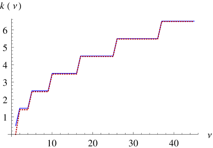
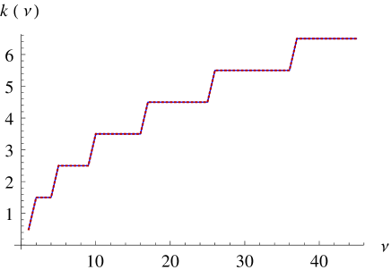
(a)		(b)
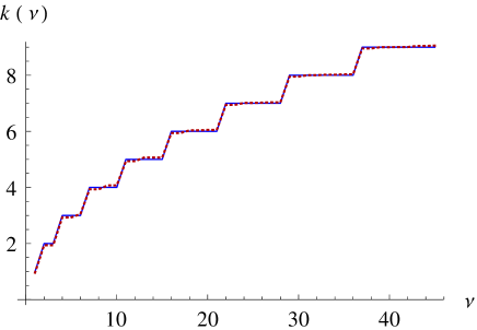
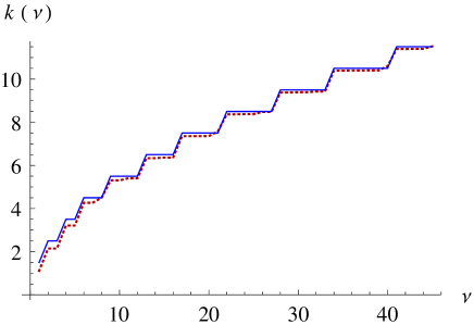
(c)		(d)

Figure 1: Comparison of the spectra of several AIs calculated with the WKB method (blue line) with the analytically or numerically calculated spectra (red dashed line). The spectra are represented by the function $k(\nu)$, degenerate levels correspond to plateaus in the graph. (a) Maxwell’s fish eye, (b) Kepler profile, (c) Miñano lens, (d) a 2D AI with the refractive index $n(r)=2r^{-1}\{[(2-r)/r]^{3/2}+[r/(2-r)]^{3/2}\}^{-1}$. In (b), the analytical and WKB spectra are identical.

5 Mirrors

So far we have considered absolute instruments without mirrors, so we required the wave in the evanescent region to decay gradually. However, in many AIs there are mirrors that constitute their important parts. The mirrors play one or both of the following two roles. First, in some AIs they limit the size of the device, e.g. from infinite size to a finite one. This is the case of Maxwell’s fish eye mirror (MFEM) [6, 4]. The second possible role is that mirrors can eliminate regions where the refractive index goes to zero; this is again the case of MFEM or e.g. of the modified Miñano lens [4].

Consider a situation that there is a spherical (or in 2D, circular) mirror at radius $r=b$ in the AI. Due to the boundary condition the wave has to vanish at it, i.e., $w(b)=0$. We have to distinguish two cases: either the mirror is placed in the evanescent or in the oscillatory region. In the following we will treat them separately.

5.1 Mirror in the evanescent region

Suppose first that the mirror is placed in the evanescent region, e.g. $b>r_{+}$. Then for $r>r_{+}$ we need not only the exponentially decaying solution in Eq. (11) but also the exponentially growing one to create their superposition that vanishes at $r=b$. This will cause a phase shift of the wave in the oscillatory region and consequently a shift in the spectrum compared to the situation without the mirror.

To describe such a situation, we will use one of the standard methods for matching the WKB solutions in the oscillatory and evanescent regions employing Airy functions. For this purpose we approximate the bracket in Eq. (6), i.e., $p^{2}$, by a linear function of $r$ in the vicinity of the turning points. To write this explicitly for the turning point $r_{+}$, we put $p^{2}(r)\approx-\alpha(r-r_{+})$, for which Eq. (6) has exact solutions $w_{1}(r)=\operatorname*{Ai}(\alpha^{1/3}(r-r_{+}))$ and $w_{2}(r)=\operatorname*{Bi}(\alpha^{1/3}(r-r_{+}))$ (up to a multiplicative constant). Using the asymptotic formulas for Airy functions [17] that are very accurate for $|x|\gtrsim 2$, namely

$$\operatorname*{Ai}(x)\approx\begin{cases}\pi^{-1/2}(-x)^{-1/4}\sin[\frac{2}{3}(-x)^{3/2}+\pi/4]&(x<0)\\ \frac{1}{2}\pi^{-1/2}x^{-1/4}\exp(-\frac{2}{3}x^{3/2})&(x>0)\end{cases}$$ (24)

and

$$\operatorname*{Bi}(x)\approx\begin{cases}\pi^{-1/2}(-x)^{-1/4}\cos[\frac{2}{3}(-x)^{3/2}+\pi/4]&(x<0)\\ \pi^{-1/2}x^{-1/4}\exp(\frac{2}{3}x^{3/2})&(x>0)\end{cases}$$ (25)

we can express the solutions $w_{1,2}(r)$ for $r<r_{+}$ as

$$w_{1}(r) \approx \frac{\alpha^{1/6}}{\sqrt{\pi p}}\cos\left(\int_{r_{+}}^{r}p(r^{\prime})\,{\rm d}r^{\prime}+\frac{\pi}{4}\right)$$ (26)

$$w_{2}(r) \approx \frac{\alpha^{1/6}}{\sqrt{\pi p}}\sin\left(\int_{r_{+}}^{r}p(r^{\prime})\,{\rm d}r^{\prime}+\frac{\pi}{4}\right)\,,$$ (27)

where the linearisation of $p^{2}$ was used again to write the expressions $(\pm x)^{3/2}$ in Eqs. (24) and (25) as integrals of $p$. Obviously, the solutions (26) and (27) can be expressed as linear combinations of the solutions (11) in the oscillatory region. This way Eqs. (26) and (27) describe the same solutions as Eq. (11), and a similar consideration can be made for the evanescent region. This allows us to express the approximate solutions of Eq. (6) in the evanescent and oscillatory regions as well as in the vicinity of the turning point $r_{+}$ by a single formula using the Airy functions Ai and Bi. Their argument is obtained by expressing the $x$ variable in Eqs. (24) and (25) in terms of the integral of $p$ with the help of Eqs. (26) and (27). This way we arrive at the following approximate solutions of Eq. (6):

$$f_{1}(r)=\operatorname*{Ai}\left[-\sqrt[3]{\left(\frac{3}{2}\int_{r}^{r_{+}}p\,{\rm d}r\right)^{2}}\right],\quad f_{2}(r)=\operatorname*{Bi}\left[-\sqrt[3]{\left(\frac{3}{2}\int_{r}^{r_{+}}p\,{\rm d}r\right)^{2}}\right]\,.$$ (28)

In this expression the integral is real or purely imaginary for $r<r_{+}$ or $r>r_{+}$, respectively. Its square in these regions is positive or negative, respectively, and so is the third root. It is easy to check that if $p^{2}(r)=-\alpha(r-r_{+})$, then the brackets in Eq. (28) turn into $\alpha^{1/3}(r-r_{+})$ for all $r$, so in that case Eqs. (28) represent the exact solutions. Moreover, even if $p^{2}(r)$ is non-linear, Eqs. (28) still provide a very good approximation to the solutions of Eq. (6). Most importantly, the positions of the nodes match very well the positions of the nodes of the exact solution. This can be seen on the examples in Figs. 2 and 3.

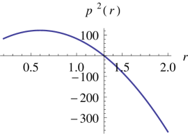
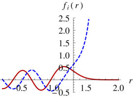
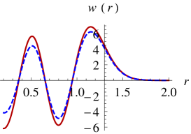
(a)		(b)		(c)

Figure 2: Example of the functions relevant for describing the approximate solutions of Eq. (6). (a) The function $p^{2}(r)$ chosen to be significantly non-linear, (b) the corresponding functions $f_{1}(r)$ (red) and $f_{2}(r)$ (dashed blue) from Eqs. (28). In (c) we compare a numerical solution of Eq. (6) satisfying $w(2)=0,w^{\prime}(2)=-0.02$ (red curve) with its approximate solution in terms of a superposition of the functions $f_{1}(r),f_{2}(r)$ (dashed blue curve) satisfying the same conditions. The agreement between the two curves is very good, in particular the position of the nodes that has the key importance for the spectrum. The $y$-axis of the graphs is placed at the turning point $r_{+}$ (in this case $r_{+}=1.3$).

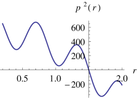
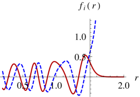
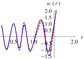
(a)		(b)		(c)

Figure 3: As in Fig. 2, but with an even stronger non-linearity of the function $p(r)^{2}$, and the parameters $r_{+}=1.5$, $w(0.5)=1,w^{\prime}(0.5)=-1$.

Eqs. (28) enable to find the phase of the wave in the oscillatory region very accurately. What we have to do is to find the coefficients $c_{1,2}$ such that the superposition $w(r)=c_{1}f_{1}+c_{2}f_{2}$ satisfies the condition $w(b)=0$. The solution is, up to a common multiplicative factor, $c_{1}=\operatorname*{Bi}(\xi)$ and $c_{2}=-\operatorname*{Ai}(\xi)$, where $\xi=-\sqrt[3]{\left(\frac{3}{2}\int_{b}^{r_{+}}p\,{\rm d}r\right)^{2}}$. Using the asymptotic forms (26), (27) in the oscillatory region, we find that in this region

$$w(r)\approx\frac{\mbox{const}}{\sqrt{p}}\cos\left(\int_{r_{+}}^{r}p(r^{\prime})\,{\rm d}r^{\prime}+\eta\right)\,,$$ (29)

with the phase shift

$$\eta=\arctan\frac{\operatorname*{Bi}(\xi)-\operatorname*{Ai}(\xi)}{\operatorname*{Bi}(\xi)+\operatorname*{Ai}(\xi)}\,$$ (30)

The difference between $\eta$ and $\pi/4$ gives a correction factor for Eqs. (18) and (19) that has to be added to the curly parentheses. A similar consideration can be made in the situation when there is a mirror in the other evanescent region $r<r_{-}$. Naturally, the closer the turning point is to the mirror, the larger will be the correction. This way the largest shifts will be exhibited by the levels corresponding to the smallest values of $m$.

Fig. 4 shows the results of our method on two examples of AIs where the mirror has been placed at the boundary of the classically accessible region at $r=b=2$. The first one is the Kepler profile, the second one is Miñano lens. The WKB spectrum is compared with the numerically calculated spectrum. The difference is so small that it can be hardly seen in the pictures. For comparison, the WKB spectrum in the absence of the mirror is also shown. The mirror obviously shifts all the levels up as could be expected. A closer inspection of the spectrum reveals that the shift indeed decreases with increasing $m$ due to the increasing separation of the turning point from the mirror.

Fig. 4 also clearly reveals that the spectrum is no more so degenerate as it was in the absence of the mirror. As was shown in [4], the regularity and degeneracy of the spectrum is connected with the quality of imaging by the device, so adding the mirror degrades somewhat the imaging, in particular at low frequencies. Note that this happens even though the mirror is situated beyond the turning point $r_{+}$ for most rays (i.e., for all rays with the exception of the ones with $L=0$ for which the mirror is just at the turning point). In terms of geometrical optics, nothing changes when the mirror is added because only the rays with $L=0$ reach it, and even their trajectory remains unchanged. However, unlike the rays, the wave “feels” the mirror even if it is located in the evanescent, i.e., classically inaccessible region.

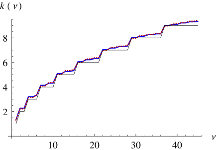
(a)		(b)

Figure 4: Comparison of the WKB spectra (blue) and numerically calculated spectra (dashed red) for two AIs with mirrors. (a) Kepler index profile surrounded by a mirror at radius $b=2$. (b) Miñano profile surrounded by a mirror at radius $b=2$. The difference between the curves can be hardly seen, the relative errors make a few per cent even for the lowest levels and becomes completely negligible for higher frequencies. The thin black lines show the WKB spectra of the corresponding devices without the mirror.

5.2 Mirror in the oscillatory region

We will now consider the situation when the mirror is not in the evanescent, but rather in the oscillatory region, which is the case e.g. of Maxwell’s fish eye mirror. Suppose that the optical medium is inside the mirror, again as in the case of MFEM. The upper turning point $r_{+}$ is then located at the mirror itself, so $w(r)$ must vanish there and so for $r<r_{+}$ the wave must behave according to Eq. (29) with $\eta=\pi/2$. This means an additional constant phase factor of $\pi/4$ compared to Eq. (12), which then has to be added into the curly parentheses in Eqs. (18) and (19). Applying this result to the 2D MFEM (for which $n(r)=2/(1+r^{2})$, $\mu=2$ and $b=1$), we get for the WKB spectrum

$$k_{\rm WKB}=2N+|m|+3/2\,.$$ (31)

The analytical form of the spectrum is

$$k_{\rm analytic}=\sqrt{(2N+|m|+1)(2N+|m|+2)}\,.$$ (32)

This way, the WKB method gives here very good results in a similar way as for the simple Maxwell’s fish eye.

6 Conclusions

In this paper we have developed a method for calculating frequency spectra of absolute instruments using the WKB approximation. Our method is based on a the key relation (15) between the optical path $S$ and the semiclassical phase change $\Phi$ between the turning points, and on the fact that in AIs of the first type the optical path $S$ is independent of the angular momentum. The method proved to be very efficient for describing the spectrum accurately even for the lowest levels. The results confirmed the previously derived properties of the spectra, in particular that the frequencies are strongly degenerate in AIs and that they form almost equidistantly spaced groups. Since these properties of the spectrum have key importance for focusing of waves by AIs [13], the WKB method shows that sharp focusing of rays in fact implies that waves will be focused as well. This way the WKB method provides a nice and important bridge between geometrical and wave optics of absolute instruments.

We applied our method also to AIs that contain mirrors; there, the Airy functions turned out to be very helpful in describing the wave in both the oscillatory and evanescent regions, and to calculate the eigenfrequency shifts caused by the mirror. When the mirror is added into the evanescent region, it turns out that even though light rays are not influenced at all, the spectrum can be influenced strongly. In particular, the spectrum becomes less regular, which can somewhat degrade imaging by the absolute instrument. On the other hand, placing the mirror in the oscillatory region leads to a constant shift in the spectrum.

It may be somewhat surprising, but certainly very satisfactory, how accurate results the WKB method gives for the spectra of absolute instruments. The situation is similar to quantum mechanics where the WKB method also gives very precise values for the energy spectrum in many situations. An interesting question for further research could be how the WKB method can be applied to AIs of the second type where not all points have their full images, or to even more general devices.

References

- [1] Born M and Wolf E 2006 Principles of optics (Cambridge: Cambridge University Press)
- [2] Maxwell J C 1854 Camb. Dublin Math. J. 8 188
- [3] Miñano J C 2006 Opt. Express 14 9627
- [4] Tyc T, Herzánová L, Šarbort M and Bering K 2011 New J. Phys. 13 115004
- [5] Tyc T 2011 Phys. Rev. A 84 031801(R)
- [6] Leonhardt U 2009 New J. Phys. 11 093040
- [7] Ma Y G, Sahebdivan S, Ong C K, Tyc T and Leonhardt U 2011 New J. Phys. 13 033016
- [8] Ma Y G, Sahebdivan S, Ong C K, Tyc T and Leonhardt U 2012 New J. Phys. 14 025001
- [9] Blaikie R J 2010 New J. Phys. 12 058001
- [10] Leonhardt U 2010 New J. Phys. 12 058002
- [11] Tyc T and Zhang X 2011 Nature 480 42
- [12] Quevedo-Teruel O, Mitchell-Thomas R C and Hao Y 2012 Phys. Rev. A 86 053817
- [13] Tyc T and Danner A 2012 New J. Phys. 14 085023
- [14] Langer R E 1934 Bull. Am. Math. Soc. 40 545
- [15] Berry M V and Mount K E 1972 Rep. Prog. Phys. 35 315
- [16] Landau L D and Lifshitz E M 1991 Quantum mechanics (Pergamon Press)
- [17] Vallée O and Soares M 2004 Airy functions and applications to physics (London: Imperial College Press)