Link-disorder fluctuation effects on synchronization in random networks

Abstract

We consider one typical system of oscillators coupled through disordered link configurations in networks, i.e., a finite population of coupled phase oscillators with distributed intrinsic frequencies on a random network. We investigate collective synchronization behavior, paying particular attention to link-disorder fluctuation effects on the synchronization transition and its finite-size scaling (FSS). Extensive numerical simulations as well as the mean-field analysis have been performed. We find that link-disorder fluctuations effectively induce uncorrelated random fluctuations in frequency, resulting in the FSS exponent $\bar{\nu}=5/2$, which is identical to that in the globally coupled case (no link disorder) with frequency-disorder fluctuations.

I I. Introduction

Recently, it has been reported that disorder fluctuations play a crucial role on the critical scaling near the onset of synchronization, even in the mean-field (MF) regime ref:Hong_Entrainment ; ref:gl_noiseless ; ref:Daido . In particular, one recent study on the collective synchronization in the system of globally coupled oscillators (Kuramoto model) reports that “sample-to-sample fluctuations” induced by different realizations of intrinsic random frequencies yield significantly different finite-size scaling (FSS) from the ordinary MF prediction ref:Hong_Entrainment . The anomalous fluctuations are characterized by the FSS exponent $\bar{\nu}=5/2$ ref:Hong_Entrainment . When the random disorder in distributed intrinsic frequencies is completely removed, fluctuations are still anomalous but much weaker ($\bar{\nu}\simeq 5/4$) ref:gl_noiseless , because dynamic (temporal) fluctuations dominate in this case. We call the latter as the noiseless frequency distribution, while the former as the noisy frequency distribution.

When the system is put on a complex network, we need to consider another kind of fluctuations, i.e., “link-disorder fluctuations” induced by different configurations of connectivity among vertices in the network. Considering that many systems in nature are based on a complex network topology, it would be interesting to investigate how the link-disorder fluctuations affect the collective behavior of a given system in general. Most of collective behaviors invoking phase transitions in networks belong to the conventional MF class where dynamic (thermal) MF fluctuations are dominant, thus sample-to-sample disorder fluctuations become usually irrelevant ref:Hong_Entrainment ; ref:Critical_phenomena_complex_networks_RMP ; ref:sync_network_MF ; ref:SFN_sync_Hong ; ref:Ising_network_MF ; ref:XY_network_MF ; ref:phenomenology_critical_behavior_in_network ; ref:Finite_size_scaling_network ; ref:Finite_size_scaling_network_fractal_properties . However, in the presence of additional distributed quantities at vertices, link-disorder fluctuations would generate effective disorder fluctuations in distributed quantities, which might yield non-MF fluctuations.

In this study, we consider the system of coupled oscillators on a sparse link-disordered network. To separate out the effects of uncorrelated random link-disorder fluctuations, we focus on the system with a noiseless intrinsic frequency distribution on the Erdös-Rényi (ER) random and $z$-regular network ref:Erdos . The FSS property is investigated through the phase synchronization order parameter in extensive numerical simulations and the value of the FSS exponent $\bar{\nu}$ is estimated. We find that $\bar{\nu}\simeq 5/2$, which is identical to that of the globally coupled model with the noisy frequency distribution. This implies that the random link-disorder fluctuations effectively generate random and independent disorder in the frequency distribution. It is also found that the addition of random disorder in the intrinsic frequency distribution (noisy case) on the ER network does not change the FSS exponent.

The present paper is outlined as follows. In Sec. II we introduce the model, and explain how we generate the noiseless frequency distribution. In Sec. III, we present the mean-field (MF) analysis on the ER network with the predictions on the order parameter exponent $\beta$ and the FSS exponent $\bar{\nu}$. Section IV shows numerical simulation results. A brief summary is given in Sec. V.

II II. Model

We begin with a finite population of $N$ coupled phase oscillators on a sparse network. To each vertex $i$ of the network, we associate an oscillator whose state is described by the phase $\phi_{i}$ governed by the equation of motion

$$\dot{\phi}_{i}=\omega_{i}-K\sum_{j=1}^{N}a_{ij}\sin(\phi_{i}-\phi_{j}),$$ (1)

where $\omega_{i}$ represents the intrinsic frequency of the $i$th oscillator. It is assumed that $\{\omega_{i}\}$ are distributed according to a symmetric and unimodal distribution function $g(\omega)$ such as a Gaussian one with zero mean $(\langle\omega\rangle=0)$ and finite variance $(\langle\omega_{i}\omega_{j}\rangle=\sigma^{2}\delta_{i}\delta_{j})$. The $\{a_{ij}\}$ denotes the adjacency matrix defined by

$$a_{ij}=\left\{\begin{array}[]{ll}1,&{\mbox{ when}}~{}{i~{}{\mbox{and}}~{}j~{}{\mbox{are~{}linked}}},\\ 0,&{\mbox{otherwise}},\end{array}\right.$$ (2)

and the degree $k_{i}$ of the vertex $i$ is defined as the number of vertices linked to $i$, i.e. $k_{i}=\sum_{j}a_{ij}$. In a sparse network, the total number of links is proportional to $N$. The second term on the right-hand side of Eq. (1) represents ferromagnetic coupling to neighboring oscillators on the network ($K>0$), so the neighboring oscillators favor their phase difference minimized.

When the coupling is weak (small $K$), each oscillator tends to evolve with its own dynamics described by $d\phi_{i}/dt\simeq\omega_{i}$, showing no synchrony. As the coupling is increased, the oscillators interact with each other and eventually a macroscopic number of synchronized oscillators can appear if the coupling is strong enough. Emergence of macroscopic synchronization can be probed by the phase order parameter ref:Kuramoto

$$\Delta e^{i\theta}=\frac{1}{N}\sum_{j=1}^{N}e^{i\phi_{j}},$$ (3)

where $\Delta$ measures the magnitude of the phase synchrony and $\theta$ denotes the average phase.

Near the synchronization transition ($\Delta\approx 0$), the MF analysis shows that the order parameter $\Delta$ vanishes with the ordinary MF exponent $\beta=1/2$, if the degree distribution $\{k_{i}\}$ is not strongly heterogeneous ref:sync_network_MF ; ref:SFN_sync_Hong . The ER random network has an exponential degree distribution with weak heterogeneity, thus the ordinary MF exponent should be found.

The FSS is governed by fluctuations. In the system described by Eq. (1), there could be three different fluctuations. One comes from dynamic (temporal) fluctuations which persist even in the steady state due to the presence of running (non-static) oscillators. Two others are due to quenched disorder in link configurations $\{a_{ij}\}$ in a sparse network and possibly in frequency distributions $\{\omega_{i}\}$ obtained by a random drawing procedure from the distribution $g(\omega)$. It is difficult to study analytically the dynamic fluctuations even in the globally coupled case (no link disorder) and there still exists a controversy ref:gl_noiseless ; ref:Daido . However, it is known that frequency-disorder fluctuations dominate over dynamic fluctuations at least in the globally coupled case ref:Hong_Entrainment ; ref:gl_noiseless .

In this work, we focus on the effects of link-disorder fluctuations separately, so that we need to remove frequency-disorder fluctuations completely from the system. This can be achieved by generating the frequencies $\{\omega_{i}\}$ following a deterministic procedure given by ref:gl_noiseless

$$\frac{i-0.5}{N}=\int_{-\infty}^{\omega_{i}}g(\omega)d\omega.$$ (4)

The generated frequencies are quasi-uniformly spaced in accordance with the distribution $g(\omega)$ in the population. As this noiseless frequency set is uniquely determined, there is no disorder originating from different realizations of frequencies. For the globally coupled model with this noiseless set, dynamic fluctuations dominate the FSS with the weak FSS exponent $\bar{\nu}\simeq 5/4$ ref:gl_noiseless , in contrast that $\bar{\nu}=5/2$ ref:Hong_Entrainment with disorder in frequency sets by randomly and independently drawing frequencies from the distribution $g(\omega)$.

The question we raise in this work is what kind of FSS emerges in a sparse network such as the ER network with the noiseless frequency set, i.e. what is the role of disorder in link configurations? Also does the FSS change or not if disorder in frequency sets is added in the ER network? In the following sections, we start with a MF analysis and report extensive numerical results.

III III. Mean-field analysis

We consider the ER networks as simple examples of uncorrelated random sparse networks. In the ER random network, any pair of vertices is linked independently with probability $z/N$. In the large $N$ limit, the average degree becomes $\langle k\rangle=z$ and the degree distribution is given by the Poisson distribution ref:Erdos ; ref:Newman

$$P(k)=\frac{\langle k\rangle^{k}e^{-\langle k\rangle}}{k!}.$$ (5)

In the $z$-regular random network, all vertices have the same degree $z$ with random connectivity between vertices, so the degree distribution is given by the Kronecker $\delta$-function as $P(k)=\delta_{k,z}$.

Taking the annealed MF approximation for connectivity of the network $a_{ij}\approx k_{i}k_{j}/N\langle k\rangle$ (heterogeneous MF theory), one can introduce the global ordering field $H\exp(i\theta)$ ref:SFN_sync_Hong as

$$He^{i\theta}=\frac{1}{N}\sum_{j}\frac{k_{j}}{\langle k\rangle}e^{i\phi_{j}},$$ (6)

and then the equation of motion, Eq. (1), can be rewritten as

$$\dot{\phi}_{i}=\omega_{i}-k_{i}KH\sin(\phi_{i}-\theta).$$ (7)

In the long-time limit where the global ordering field approaches a constant in average, one can easily solve Eq. (7) for each $\phi_{i}$ with a constant $H$ and $\theta$. Then, we can set up the self-consistency equation for $H$ through Eq. (6) as

$$H=\frac{1}{N}\sum_{j=1}^{N}\frac{k_{j}}{\langle k\rangle}\sqrt{1-\Bigl{(}\frac{\omega_{j}}{k_{j}KH}\Bigr{)}^{2}}\Theta\Bigl{(}1-\frac{|\omega_{j}|}{k_{j}KH}\Bigr{)},$$ (8)

where $\Theta(x)$ is the Heaviside step function, which takes the value $1$ for $x\geq 0$ and $0$ otherwise. Each term inside the summation represents the contribution from an oscillator with $\omega_{j}$ at vertex $j$ with degree $k_{j}$. Note that only entrained oscillators with $|\omega_{j}|<k_{j}KH$ contribute.

The frequency set $\{\omega_{i}\}$ fluctuates randomly over the samples for the noisy frequency distribution, and the degree configuration $\{k_{i}\}$ also fluctuates randomly for the ER random network. Thus, the nontrivial (nonzero $H$) solution of the self-consistent equation also fluctuates over the samples. With either one of fluctuations, we expect the Gaussian fluctuations for sufficiently large $N$ from the central limit theorem, and the self-consistency equation for small $H$ becomes ref:SFN_sync_Hong

$$H=(K/K_{c})H-c(KH)^{3}+d(KH)^{1/2}N^{-1/2}\xi$$ (9)

with $K_{c}=[2/\pi g(0)]\langle k\rangle/{\langle k^{2}\rangle}$, and constants $c=-[{\pi g^{{}^{\prime\prime}}(0)}/{16}]{\langle k^{4}\rangle}/{\langle k\rangle}$ and $d=\sqrt{[4g(0)/3]{\langle k^{3}\rangle}/{\langle k^{2}\rangle}}$. The term $\xi$ is a Gaussian random variable with zero mean and unit variance, which represents frequency-disorder fluctuations and/or link-disorder fluctuations.

The scaling solution to Eq. (9) can be easily obtained in the FSS form ref:SFN_sync_Hong ; ref:Fisher

$$H=N^{-1/5}f[(K-K_{c})N^{2/5}],$$ (10)

implying $\beta/\bar{\nu}=1/5$ and $\bar{\nu}=5/2$. We note that this result is the same as that of the globally coupled noisy oscillators with frequency-disorder fluctuations ref:Hong_Entrainment ; ref:gl_noiseless .

One exceptional case can be constructed when the system is put on the $z$-regular random network with the noiseless frequency set. In the present MF scheme, there is no fluctuation in the solution of $H$ and one may expect the same FSS behavior as that of the globally coupled noiseless oscillators with $\beta/\bar{\nu}\approx 2/5$ and $\bar{\nu}\approx 5/4$, representing dynamic fluctuations only. However, the MF approximations ignore fluctuations in connectivity disorder (absent for the globally coupled case), which might give rise to another type of sample-to-sample Gaussian fluctuations dominant over dynamic fluctuations.

In the next section, we check the validity of the MF analysis via extensive numerical simulations in the ER random and $z$-regular networks with the noiseless and noisy frequency distributions.

IV IV. Numerical analysis

We perform extensive numerical simulations for the system governed by Eq. (1). The ER and the $z$-regular random networks are generated for the average degree $z=\langle k\rangle=6$ up to the system size $N=12800$. For the noiseless frequency distribution, we generate the intrinsic frequencies by the process shown in Eq. (4) with $g(\omega)=(2\pi\sigma)^{-1/2}\exp(-\omega^{2}/2\sigma^{2})$ with unit variance $(\sigma^{2}=1)$. We used Heun’s method ref:Heun , with a discrete time step $\delta t=0.01$, in the numerical integration of Eq. (1) up to $4\times 10^{4}$ time steps. Initial values for $\{\phi_{i}(0)\}$ are chosen random, and data are collected only for the latter half of time steps to avoid any transient behavior exp . For each network size, we also average the data over $10^{2}\sim 10^{3}$ different realizations of the network.

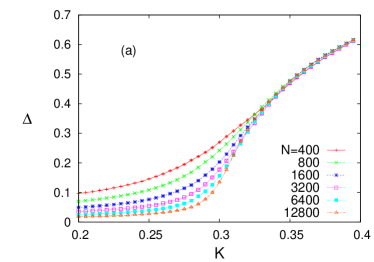
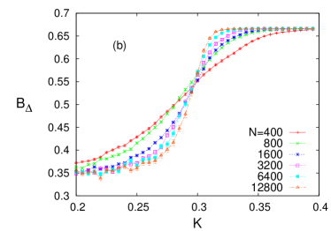
Figure 1: (Color online) (a) The order parameter $\Delta$ is plotted as a function of the coupling strength $K$ for various system size $N$. (b) Binder cumulant $B_{\Delta}$ versus $K$ for various system size $N$, where we estimate $K_{c}=0.300(5)$ from the crossing points.

First, we consider the ER random network and measure the phase order parameter $\Delta$ as a function of the coupling constant $K$ for various system size $N$, see Fig. 1 (a). The critical coupling strength $K_{c}$, beyond which the phase synchronization occurs, can be accurately located by utilizing the Binder cumulant ref:HPT-BC

$$B_{\Delta}=1-\Biggr{[}\frac{\overline{\Delta^{4}}}{3\overline{\Delta^{2}}^{2}}\Biggr{]},$$ (11)

where the overbar represents the time average after sufficient relaxation and $[\cdots]$ represents the average over different realizations of the networks, respectively. In the weak coupling regime $K\ll K_{c}$, the Binder cumulant $B_{\Delta}$ goes to $1/3$ in the large $N$ limit, while it goes to $2/3$ for the strong coupling regime $(K\gg K_{c})$. The Binder cumulant curves with different $N$ cross each other at the critical coupling strength $K_{c}$, as seen in Figure 1 (b). We estimate $K_{c}=0.300(5)$ by extrapolating the crossing points in the large $N$ limit. Note that the MF prediction on $K_{c}$ is about $0.23$ in Eq. (9), which is quite far away from the numerical estimate. It is not surprising to see a considerable shift of the critical point, because the inherent linking disorder in the quenched networks generates finite correlations in neighboring nodes. However, it is hoped that the scaling nature near the transition is not affected by finite correlations, since is is usually universal.

We now check the FSS relation of Eq. (10). As one can easily show $\Delta\propto H$ for small $H$ at the MF level ref:SFN_sync_Hong , we expect

$$\Delta N^{1/5}={\tilde{f}}[(K-K_{c})N^{2/5}],$$ (12)

where the scaling function ${\tilde{f}}[x]$ is characterized by

$${\tilde{f}}[x]\sim\left\{\begin{array}[]{ll}{\mbox{const}},&x=0,\\ x^{1/2},&x>0,\\ (-x)^{-3/4},&x<0\end{array}\right.$$ (13)

for the ER random networks with the noiseless frequency distribution. Figure 2 shows the scaling function ${\tilde{f}}[x]$ by collapsing the order parameter data for various different sizes, using the exponents $\beta/\bar{\nu}=1/5$ and $\bar{\nu}=5/2$, which agrees perfectly with the MF prediction of the exponent values. Figure 3 is the scaling plot for the ER random networks with the noisy frequency distribution. As expected, the scaling collapse is found with the same values of the exponents $\beta/\bar{\nu}=1/5$ and $\bar{\nu}=5/2$. Moreover, the scaling function ${\tilde{f}}[x]$ is identical for both the noiseless and noisy distributions with the same critical coupling strength $K_{c}$. Differences can be seen only in higher-order finite-size effects.

We also report the scaling plot for the $z$-regular random network with the noiseless frequency distribution in Fig. 4. As the strength of neighboring correlations in quenched networks depends on the details of networks, the critical point in the $z$-regular network is located differently from that in the ER random network, which is estimated as $K_{c}=0.365(5)$ from the Binder cumulant analysis. Nevertheless, the corresponding exponent values of $\beta/\bar{\nu}$ and $\bar{\nu}$ are identical to those in the ER random network as shown in Fig. 4, which are against the MF prediction discussed in the previous section. This implies that the random link-disorder fluctuations in the quenched $z$-regular network generate sample-to-sample Gaussian fluctuations of the same kind in the ER random networks as well as in the globally coupled network with frequency-disorder fluctuations. However, the scaling function ${\tilde{f}}[x]$ by itself is distinct from that in the ER networks.

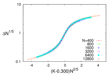
Figure 2: (Color online) Scaling plot of $\Delta$ for various system size $N$ in the ER random networks with the noiseless frequency distribution.

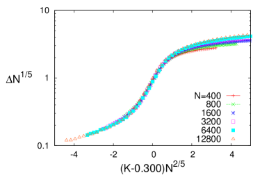
Figure 3: (Color online) Scaling plot of $\Delta$ for various system size $N$ in the ER random networks with the noisy frequency distribution.

Figure 4: (Color online) Scaling plot of $\Delta$ for various system size $N$ in the $z$-regular random networks with the noiseless frequency distribution.

V V. Summary

In this work, we considered a finite population of coupled random frequency oscillators on the ER and the $z$-regular random network with link-disorder fluctuations. In the globally coupled network without any link disorder, the finite-size fluctuations are determined crucially by the existence of disorder in the intrinsic frequency distribution. Under the presence of link disorder in random networks, we find that the finite-size fluctuations are universal with the anomalous FSS exponent $\bar{\nu}=5/2$, independent of the details of the degree distribution (if not strongly heterogeneous) and also independent of the frequency disorder. We note, however, that the scaling function is not universal, depending on the details of the network connectivity.

VI Acknowledgment

This work was supported by the Mid-career Researcher Program through the NRF Grant No. 2010-0026627 (H.P.) and the Basic Science Research Program through No. 2012R1A1A2003678 (H.H.) funded by MEST.

References

- (1) H. Hong, H. Chaté, H. Park, and L.-H. Tang, Phys. Rev. Lett. 99, 184101 (2007); H. Hong, H. Park, and M. Y. Choi, Phys. Rev. E 72, 036217 (2005).
- (2) H. Hong, H. Park, L. -H. Tang, and H. Chaté (to be published).
- (3) H. Daido, Prog. Theor. Phys. 75, 1460 (1986); ibid. 77, 622 (1987).
- (4) For a review, see S. N. Dorogovtsev, A. V. Goltsev, and J. F. F. Mendes, Rev. Mod. Phys. 80, 1275 (2008), and references therein.
- (5) H. Hong, M. Y. Choi, and B. J. Kim, Phys. Rev. E 65, 026139 (2002); T. Ichinomiya, Phys. Rev. E 70, 026116 (2004); ibid., 72, 016109 (2005); D.-S. Lee, Phys. Rev. E 72, 026208 (2005); T. Ichinomiya, Prog. Theor. Phys. 113, 1 (2005); J. Gómez-Gardeñes, Y. Moreno, and A. Arenas, Phys. Rev. E 75, 066106 (2007); Phys. Rev. Lett. 98, 034101 (2007).
- (6) H. Hong, H. Park, and L.-H. Tang, Phys. Rev. E 76, 066104 (2007).
- (7) A. Barrat and M. Weight, Eur. Phys. J. B 13, 547 (2000); C. P. Herrero, Phys. Rev. E 65, 066110 (2002); M. B. Hastings, Phys. Rev. Lett. 91, 098701 (2003); C. P. Herrero, Phys. Rev. E 69, 067109 (2004); J. Viana Lopes, Y. G. Pogorelov, J. M. B. Lopes dos Santos, and R. Toral, Phys. Rev. E 70, 026112 (2004).
- (8) B. J. Kim, H. Hong, P. Holme, G. S. Jeon, P. Minnhagen, and M. Y. Choi, Phys. Rev. E 64, 056135 (2001); K. Medvedyeva, P. Holme, P. Minnhagen, and B. J. Kim, Phys. Rev. E 67, 036118 (2003); A. C. C. Coolen, N. S. Skantzos, I. P. Castillo, C. J. P. Vicente, J. P. L. Hatchett, B. Wemmenhove, and T. Nikoletopoulos, J. Phys. A 38, 8289 (2005).
- (9) A. V. Goltsev, S. N. Dorogovtsev, and J. F. F. Mendes, Phys. Rev. E 67, 026123 (2003).
- (10) H. Hong, M. Ha, and H. Park, Phys. Rev. Lett. 98, 258701 (2007).
- (11) C. Song, S. Havlin, and H. A. Makse, Nature Physics 2, 275 (2006); K. -I. Goh, G. Salvi, B. Kahng, and D. Kim, Phys. Rev. Lett. 96, 018701 (2006); L. K. Gallos, C. Song, S. Havlin, and H. A. Makse, PNAS 104, 7746 (2007).
- (12) P. Erdös and A. Rényi, Publicationes Mathematicae Debrencen 6, 290 (1959).
- (13) Y. Kuramoto, in Proceedings of the International Symposium on Mathematical Problems in Theoretical Physics, edited by H. Araki (Springer-Verlag, New York, 1975); Chemical Oscillations, Waves, and Turbulence (Springer-Verlag, Berlin, 1984); Y. Kuramoto and I. Nishikawa, J. Stat. Phys. 49, 569 (1987).
- (14) M. E. J. Newman, S. H. Strogatz, and D. J. Watts, Phys. Rev. E 64, 026118 (2001).
- (15) M. E. Fisher, Rep. Prog. Phys. 30, 615 (1967).
- (16) See. e.g., R. L. Burden and J. D. Faires, Numerical Analysis (Brooks-Cole, Pacific Grove, 1997), p.280.
- (17) Initial transient behavior turns out to remain only up to time steps for system size even at .
- (18) H. Hong, H. Park, and L.-H. Tang, J. Korean Phys. Soc. 49, L1885 (2006).