Exact Solutions in Massive Gravity

Abstract

Massive gravity is a good theoretical laboratory to study modifications of General Relativity. The theory offers a concrete set-up to study models of dark energy, since it admits cosmological self-accelerating solutions in the vacuum, in which the size of the acceleration depends on the graviton mass. Moreover, non-linear gravitational self-interactions, in the proximity of a matter source, manage to mimic the predictions of linearised General Relativity, hence agreeing with solar-system precision measurements. In this article, we review our work in the subject, classifying, on one hand, static solutions, and on the other hand, self-accelerating backgrounds. For what respects static solutions we exhibit black hole configurations, together with other solutions that recover General Relativity near a source via the Vainshtein mechanism. For the self-accelerating solutions we describe a wide class of cosmological backgrounds, including an analysis of their stability.

I Introduction

Can the graviton have a mass? A graviton mass breaks the diffeomorphism invariance of General Relativity (GR), but has the advantage to potentially provide a theory of dark energy that explains, in a technically natural way, the present day acceleration of our Universe. At large scales, gravity is modified with respect to GR, and the theory admits cosmological accelerating solutions in which the size of acceleration depends on the graviton mass. This way to explain cosmological acceleration is technically natural in the ’t Hooft sense, because in the limit of graviton mass going to zero one recovers the full diffeomorphism invariance of GR: hence, corrections to the size of dark energy must be proportional to the (tiny) graviton mass itself.

Not aware of all possible consequences of massive gravity for cosmology, Fierz and Pauli (FP), back in 1939, started the theoretical study of massive gravity from a field theory perspective Fierz:1939ix . They considered a mass term for linear gravitational perturbations, which is uniquely determined by requiring the absence of ghost degrees of freedom. The mass term breaks the gauge (diffeomorphism) invariance of GR, leading to a classical graviton with five degrees of freedom, instead of the two found in GR. There have been intensive studies into what happens beyond the linearized theory of FP. In 1972, Boulware and Deser (BD) found a scalar ghost mode at the nonlinear level, the so called sixth degree of freedom in the FP theory Boulware:1973my . This issue has been re-examined using an effective field theory approach, where gauge invariance is restored by introducing Stückelberg fields ArkaniHamed:2002sp . In this language, the Stückelberg fields physically play the role of the additional scalar and vector graviton polarizations. They acquire nonlinear interactions which contain more than two time derivatives, signaling the existence of a ghost ArkaniHamed:2002sp . In order to construct a consistent theory, nonlinear terms should be added to the FP model, which are tuned to remove the ghost order by order in perturbation theory. Interestingly, this approach sheds light on another famous problem with FP massive gravity; due to contributions of the scalar degree of freedom, solutions in the FP model do not continuously connect to solutions in GR, even in the limit of zero graviton mass. This is known as the van Dam, Veltman, and Zakharov (vDVZ) discontinuity vanDam:1970vg ; Zakharov:1970cc . Observations such as light bending in the solar system would exclude the FP theory, no matter how small the graviton mass is. In 1972, Vainshtein Vainshtein:1972sx proposed a mechanism to avoid this conclusion; in the small mass limit, the scalar degree of freedom becomes strongly coupled and the linearized FP theory is no longer reliable. In this regime, higher order interactions, which are introduced to remove the ghost degree of freedom, should shield the scalar interaction and recover GR on sufficiently small scales.

Until recently, it was thought to be impossible to construct a ghost-free theory for massive gravity that is compatible with current observations Creminelli:2005qk ; Deffayet:2005ys . Using an effective field theory approach, one can show that in order to avoid the presence of a ghost, interactions have to be chosen in such a way that the equations of motion for the scalar and vector component of the Stückelberg field contains no more than two time derivatives. Recently, it was shown that there is a finite number of derivative interactions for scalar lagrangians that give rise to second order differential equations. These are dubbed Galileon terms because of a symmetry under a constant shift of the scalar field derivative Nicolis:2008in . Therefore, one expects that any consistent nonlinear completion of FP contains these Galileon terms, at least in an appropriate range of scales in which the scalar dynamics can be somehow isolated from the remaining degrees of freedom; this is the so-called decoupling limit ArkaniHamed:2002sp . This turns out to be a powerful criterium for building higher order interactions with the desired properties. Indeed, following this route, de Rham, Gabadadze and Tolley constructed a family of ghost-free extensions to the FP theory, which reduce to the Galileon terms in the decoupling limit. We refer to the resulting theory as $\Lambda_{3}$ massive gravity drgt .

In this article, we review our work to build and analyze exact solutions in $\Lambda_{3}$ massive gravity. As we have briefly explained, non-linear effects play an essential role to characterize phenomenological consequences of this theory. Then, the analysis of exact solutions of the equations of motion, obtained by imposing appropriate symmetries (spherical symmetry for static space-times, or homogeneity and isotropy for cosmological set-ups), make manifest, in idealized but representative situations, how the non-linear dynamics of the graviton degrees of freedom respond to the presence of a source, or, at very large scales, to the graviton mass itself. After all, looking back to the past, we know that the knowledge of exact solutions of non-linear field equations have been of crucial importance to understand GR. The Schwarzschild solution lead to the discovery of the concept of black hole, and play an essential role for analyzing the dynamics of objects around massive sources in GR; and modern cosmology would be unthinkable without the use of Friedmann-Robertson-Walker solutions. Exact solutions in massive gravity might lead to the discovery and understanding of new features and concepts in a theory of gravitation that can lead to important developments for our comprehension of gravitational interactions.

This review is organized as follows: in Section II we explicitly construct the $\Lambda_{3}$ massive gravity theory, while in Section III the most general Ansatz for spherically symmetric solution is introduced. This leads to two branches of static solutions: one exhibiting the Vainshtein mechanism, and the other representing a generalisation of Schwarzschild-(A)dS black holes. In Section IV we explore cosmological self-accelerating solutions and their stability under perturbations. Finally, in Section V we conclude, also outlining possible directions for future research.

II Ghost-free massive gravity

We begin with the covariant Fierz-Pauli mass term in four-dimensions, given by

$$\mathcal{L}_{FP}=m^{2}\sqrt{-g}\;{\cal U}^{(2)},\qquad\qquad{\cal U}^{(2)}=\left(H_{\mu\nu}H^{\mu\nu}-H^{2}\right),$$ (1)

where $m$ is a parameter with units of mass and the tensor $H_{\mu\nu}$ is a covariantisation of the metric perturbations, namely

$$g_{\mu\nu}=\eta_{\mu\nu}+h_{\mu\nu}\,\equiv\,H_{\mu\nu}+\Sigma_{\mu\nu},\qquad\qquad\mathrm{with}\qquad\Sigma_{\mu\nu}\equiv\partial_{\mu}\phi^{\alpha}\partial_{\nu}\phi^{\beta}\eta_{\alpha\beta}.$$ (2)

The Stückelberg fields $\phi^{\alpha}$ are introduced to restore reparametrisation invariance, hence transforming as scalar from the point of view of the physical metric ArkaniHamed:2002sp . The internal metric $\eta_{\alpha\beta}$ corresponds to a non-dynamical reference metric, usually assumed to be Minkowski space-time. The dynamics of the Stuckelberg fields $\phi^{\alpha}$ are at the origin of the two features discussed in the introduction: the BD ghost excitation and the vDVZ discontinuity. With respect to the first issue, as noticed by Fierz and Pauli, one can remove the ghost excitation, to linear order in perturbations, by choosing the quadratic structure $H_{\mu\nu}H^{\mu\nu}-H^{2}$. When expressed in the Stückelberg field language, terms in the action are arranged in a such way to constraint one of the four Stuckelberg fields to be non-dynamical. However, when going beyond linear order, this constraint disappears, signaling the emergence of an additional ghost mode ArkaniHamed:2002sp . Remarkably, Ref. deRham:2010ik has shown how to construct a potential, tuned at each order in powers of $H_{\mu\nu}$, to hold the constraint and remove one of the Stückelberg fields. Even though the potential is expressed in terms of an infinite series of terms for $H_{\mu\nu}$, it can be resummed into the following finite form drgt ; Koyama:solutions

$${\cal U}=-m^{2}\left[{\cal U}_{2}+\alpha_{3}\,{\cal U}_{3}+\alpha_{4}\,{\cal U}_{4}\right],$$ (3)

where $\alpha_{n}$ are free dimensionless parameters, ${\cal U}_{n}=n!\det_{n}({\mathcal{K}})$ and the tensor ${\cal K}_{\mu}^{\ \nu}$ is defined as

$${\mathcal{K}}_{\mu}^{\ \nu} \equiv \delta_{\mu}^{\ \nu}-\left(\sqrt{g^{-1}\Sigma}\right)_{\mu}^{\ \nu}.$$ (4)

(The square root is formally understood as $\sqrt{{\cal K}}_{\mu}^{\ \alpha}\sqrt{\cal K}_{\alpha}^{\ \nu}={\cal K}_{\mu}^{\ \nu}$.) The relationship of these potentials with a determinant resides on the following property, which holds for squared real matrices and a complex number $z$

$$\det\left({\mathbb{I}}+z{\mathcal{K}}\right)=1+\sum_{n=1}^{\infty}z^{n}\det_{n}({\mathcal{K}}),$$ (5)

where each determinant can be written in terms of traces as

$$\det_{1}({\mathcal{K}}) = {\rm tr}{\mathcal{K}},$$

$$\det_{2}({\mathcal{K}}) = ({\rm tr}{\mathcal{K}})^{2}-{\rm tr}({\mathcal{K}}^{2}),$$

$$\det_{3}({\mathcal{K}}) = ({\rm tr}{\mathcal{K}})^{3}-3({\rm tr}{\mathcal{K}})({\rm tr}{\mathcal{K}}^{2})+2{\rm tr}{\mathcal{K}}^{3},$$

$$\det_{4}({\mathcal{K}}) = ({\rm tr}{\mathcal{K}})^{4}-6({\rm tr}{\mathcal{K}})^{2}({\rm tr}{\mathcal{K}}^{2})+8({\rm tr}{\mathcal{K}})({\rm tr}{\mathcal{K}}^{3})+3({\rm tr}{\mathcal{K}}^{2})^{2}-6{\rm tr}{\mathcal{K}}^{4}\,.$$

All terms $\det_{n}({\mathcal{K}})$ with $n>4$ vanish in four dimensions. If one chooses a sum of determinants of the form $\sum_{n=1}^{4}\det(\mathbb{I}+z_{n}{\mathcal{K}})-4$, one can generate each $\det_{n}({\mathcal{K}})$ term with a separate coefficient $\alpha_{n}$, provided a solution to $\sum_{i=1}^{4}z_{n}^{i}=\alpha_{n}$ exists, which is guaranteed by the Newton identities. Therefore, the massive gravity theory can be written in full as

$${\cal L}=\frac{M_{Pl}^{2}}{2}\,\sqrt{-g}\left(R-2\Lambda-m^{2}{\cal U}\right),$$ (6)

where ${\cal U}$ is given by (3) and we have introduced an additional bare cosmological constant $\Lambda$. Notice that in order to obtain the Fierz Pauli term (1) as the first order correction to GR, we have ignored the tadpole term $\det_{1}({\mathcal{K}})$.

We can write the equations of motion in a more familiar way by using the potential term (3) as the source of peculiar energy momentum tensor. In this way, the Einstein equations read

$$G_{\mu\nu}=T^{{\cal U}}_{\mu\nu},$$ (7)

where the energy momentum tensor is defined as

$$T^{{\cal U}}_{\mu\nu}\,=\frac{m^{2}}{\sqrt{-g}}\,\frac{\delta\sqrt{-g}\ {\cal U}}{\delta g^{\mu\nu}}.$$ (8)

The theory defined by (6) has Minkowski spacetime as trivial solution when $\Lambda=0$, hence one can rewrite the metric $g_{\mu\nu}$ and the scalars $\phi^{\mu}$ as deviations from flat space, namely

$$g_{\mu\nu}=\eta_{\mu\nu}+h_{\mu\nu},\qquad\qquad\phi^{\alpha}=x^{\alpha}-\pi^{\alpha},$$ (9)

where $x^{\alpha}$ are the usual cartesian coordinates spanning $\eta_{\alpha\beta}$. In what follows we will use $\phi^{\alpha}$ or $\pi^{\alpha}$, having in mind that (9) relates them. Moreover, the unitary gauge (where $\pi^{\mu}=0$) simplifies the potential (3) considerably, and we will start with this choice in what follows.

There have been intensive studies in the issue of BD ghost in this theory ghost . The general (but not universal Chamseddine:2013lid ) consensus is that there is indeed no BD ghost and the maximum number of propagation modes in this theory is five. However, this does not preclude a possibility that one of the five modes becomes a ghost around some backgrounds.

III Spherically Symmetric Solutions

In this section, we review spherically symmetric solutions in the unitary gauge by following Refs. Koyama:prl ; Koyama:solutions . The most general Ansatz with spherical symmetry, before fixing the gauge, is

$$ds^{2}\,=\,-b(t,r)^{2}\,dt^{2}+a(t,r)^{2}\,dr^{2}+2d(t,r)\,dtdr+c(t,r)^{2}d\Omega^{2},$$ (10)

where $d\Omega^{2}=d\theta^{2}+\sin^{2}\theta d\phi^{2}$, and the Stuckelberg fields have the structure

$$\phi^{0}=f(t,r),\qquad\qquad\qquad\phi^{i}=g(t,r)\frac{x^{i}}{r}.$$ (11)

We start focussing on the unitary gauge ($\pi^{\mu}=0$ or, equivalently, $f=t$ and $g=r$) and look for static solutions that do not depend, explicitly, on time. The metric ansatz (10) reduces to

$$ds^{2}\,=\,-b(r)^{2}\,dt^{2}+a(r)^{2}\,dr^{2}+2d(r)\,dtdr+c(r)^{2}d\Omega^{2}\,.$$ (12)

Furthermore, we choose to write the non-dynamical flat metric in (2) as $ds^{2}=-dt^{2}+dr^{2}+r^{2}d\Omega^{2}$. It should be noticed that this is not a coordinate choice, but a way to simplify the expressions. Indeed, we have chosen the unitary gauge, hence we are left with a theory which is not diffeomorphism invariant. Hence, in this context physics does depend on the choice of coordinates: we will further explore this fact in section IV. Any change of coordinate normally breaks the unitary gauge and switches on a non-trivial profile for the Stückelberg fields. This also implies that the static solutions considered in the unitary gauge do not provide all the spherically symmetric and static solutions in this theory. Other static solutions might exist with non-trivial Stückelberg fields turned on.

Conscious of these limitations, let us start with this gauge choice: we will relax it in what follows. We plug the previous metric into the Einstein equations (7), and observe that the Einstein tensor $G_{\mu\nu}$ satisfies the identity $d(r)\,G_{tt}+b(r)^{2}\,G_{tr}\,=\,0$, which implies the algebraic constraint $0=d(r)\,T^{{\cal U}}_{tt}+b(r)^{2}\,T^{{\cal U}}_{tr}$. This last equation implies

$$d(r)\left(c_{0}r-c(r)\right)\,=\,0\,,$$ (13)

where $c_{0}$ is a function of $\alpha_{3}$ and $\alpha_{4}$ only (see Section III.2). This constraint is solved in two possible ways, defining two branches of solutions:

$$d(r)\,=\,0\hskip 25.6073pt\text{or}\hskip 25.6073ptc(r)\,=\,c_{0}\,r\,\,.$$ (14)

In the next sections we will analyze each of these two branches separately. We will start from the diagonal one $d(r)=0$ in Section III.1, where the Vainshtein effect takes place and can be analyzed in a systematic way. Then we will proceed in Section III.2 to study the class of solutions with a non-diagonal metric and $c(r)\,=\,c_{0}\,r$, corresponding to non-asymptotically flat, Schwarzschild-(Anti)-de Sitter solutions that can be relevant to explain present-day cosmological acceleration.

III.1 Branch I: Vainshtein mechanism at work

The problem of finding exact vacuum solutions in this branch $d(r)=0$ is an open question, but we can make interesting progresses by considering perturbations (not necessarily small) from flat space. The following Ansatz is useful

$$b(r)=1+N(r)dt^{2},\qquad a(r)=\left(1+F(r)\right)^{-1/2}\qquad c(r)=\left(1+H(r)\right)^{-1}.$$ (15)

Furthermore, it is convenient to introduce a new radial coordinate $\rho=\frac{r}{1+H(r)}$, so that the linearised metric is expressed as

$$ds^{2}=-(1+n)dt^{2}+(1-f)d\rho^{2}+\rho^{2}d\Omega^{2},$$ (16)

where $f(\rho)=F\big{(}r(\rho)\big{)}-2h(\rho)-2\rho h^{\prime}(\rho)$, $n(\rho)=2N\big{(}r(\rho)\big{)}$, $h(\rho)=H\big{(}r(\rho)\big{)}$ and a prime denotes a derivative with respect to $\rho$. As discussed above, one should be careful with this change of coordinates since, after fixing a gauge, a change of frame in the metric breaks the unitary gauge and switches on the Stückelberg fields $\pi^{\mu}$. It turns out that this coordinate transformation excites the radial component of $\pi^{\mu}$, which explicitly reads $\pi^{\rho}\,=\,\rho\,h$. Therefore, from now on one can think of $h$ as geometrically corresponding to the only non-zero component of the Stückelberg field $\pi^{\mu}$. At linear order, the equations for the functions $n(\rho)$, $f(\rho)$ and $h(\rho)$ in the new variable radial $\rho$ are

$$0 = \left(m^{2}\rho^{2}+2\right)f+2\rho\left(f^{\prime}+m^{2}\rho^{2}h^{\prime}+3\,m^{2}\rho h\right),$$ (17)

$$0 = \frac{1}{2}m^{2}\rho^{2}(n-4h)-\rho\,n^{\prime}-f,$$ (18)

$$0 = f+\frac{1}{2}\rho\,n^{\prime}.$$ (19)

In this linear expansion, the solutions for $n$ and $f$ are

$$n = -\frac{8GM}{3\rho}e^{-m\rho}\,,$$ (20)

$$f = -\frac{4GM}{3\rho}(1+m\rho)e^{-m\rho}\,,$$ (21)

where we fix the integration constant so that $M$ is the mass of a point particle at the origin, and $8\pi G=M_{pl}^{-2}$. These solutions exhibit the vDVZ discontinuity, since the post-Newtonian parameter $\gamma=f/n$ is $\gamma=\frac{1}{2}(1+m\rho)$, which in the massless limit reduces to $\gamma=1/2$, in disagreement with GR predictions and solar system observations.

However, in order to understand what really happens in this limit, we must carefully analyse the behaviour of the function $h(r)$ as $m\rightarrow 0$. The study of the equations of motion for this metric component makes manifest the non-linear effects responsible for the Vainshtein mechanism. To do this, we consider scales below the Compton wavelength $m\rho\ll 1$, and at the same time ignore higher order terms in $GM$. Under these approximations, the equations of motion can still be truncated to linear order in $f$ and $n$, but since $h$ is not necessarily small, we have to keep all non-linear terms in $h$. In other words, we take the usual weak field limit for the metric fields, but keep all non-linearities in the component $h$, since we expect regions where non-linear effects in $h$ become important. As shown in Koyama:solutions , the field equations reduce to the following system of coupled equations for the fields $f$, $n$, $h$:

$$f = -2\,\frac{GM}{\rho}-(m\rho)^{2}\Big{(}h-\alpha h^{2}+\beta h^{3}\Big{)}\,,$$ (22)

$$n^{\prime} = 2\,\frac{GM}{\rho^{2}}-m^{2}\rho\,\Big{(}h-\beta h^{3}\Big{)}\,,$$ (23)

$$0 = \frac{3}{2}\,\beta^{2}\,h^{5}(\rho)-\Big{(}\alpha^{2}+2\beta\Big{)}\,h^{3}(\rho)+3\,\Big{(}\alpha+\beta A(\rho)\Big{)}\,h^{2}(\rho)-\frac{3}{2}\,h(\rho)-A(\rho)=0\,,$$ (24)

where

$$\alpha \equiv 1+3\,\alpha_{3}\,$$ (25)

$$\beta \equiv \alpha_{3}+4\,\alpha_{4}\,,$$ (26)

$$A(\rho) = \big{(}\rho_{v}/\rho\big{)}^{3}\,,$$ (27)

$$\rho_{v} \equiv \left(GM/m^{2}\right)^{\!1/3}\,.$$ (28)

Equation (24) is a quintic algebraic equation in $h$, except for the special case where $\beta=0$, where it reduces to a cubic equation. Thus, after obtaining a solution for $h$ from equation (24), one can calculate the gravitational potentials $f$ and $n$ using (22) and (23). In the particular case of $\beta=0$, it is possible to describe the solution in a simple way Koyama:prl . For large radial $\rho$ values, one can linearise the equations in $h$, recovering the solution in Eqs. (20)-(21), to first order in $m\rho$. On the other hand, the Vainshtein mechanism applies, and below the so-called Vainshtein radius, $\rho_{V}=(GMm^{-2})^{1/3}$, $h$ becomes larger than one and the non-linear terms in $h$ in eq. (24) become important, recovering GR close to a matter source. Actually, for $\rho\ll\rho_{V}$ the solution for $h$ is simply given by $|h|=\rho_{V}/(\alpha\rho)\gg 1$. The latter solution for $h$ and Eq. (24) with $\beta=0$ implies

$$2\rho n^{\prime} = \frac{2GM}{\rho}\left(1+\frac{1}{2\alpha}\left(\frac{\rho}{\rho_{V}}\right)^{2}\right),$$

$$f = -\frac{2GM}{\rho}\left(1-\frac{1}{2\alpha}\left(\frac{\rho}{\rho_{V}}\right)\right).$$ (29)

Therefore, corrections to the GR solutions are indeed small for $\rho<\rho_{V}$, as shown in the left plot of Fig. 1. Note that if we consider a finite size matter source, it was shown that there is no stable solution that interpolates from the Vainshtein region to the asymptotically flat solution, and the Vainshtein region is naturally matched onto a solution that asymptotes to a non-flat cosmological background Berezhiani:2013dw .

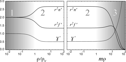
Figure 1: Numerical solution for $\partial_{r}f=f^{\prime}$, $\partial_{r}n=n^{\prime}$, and the quotient $\gamma^{\prime}\equiv f^{\prime}/2n^{\prime}$ around the Vainshtein radius $\rho_{v}$ (left) and the Compton Wavelength $\rho\sim 1/m$ (right). Region 1 (2) shows how GR solutions are (not) recovered inside (outside) the Vainshtein radius $\rho_{V}$. Region 3 shows the asymptotic decay of the linear solutions (Eqs. (20)-(21)). Here, $GM=1$ and $\alpha=1$.

For the $\beta\neq 0$ case, analytic solutions of the previous algebraic equations can not be found in general. In the following we will follow the approach presented by Ref. Koyama:Vainshtein . It is possible to determine exactly how many local solutions exist in a neighbourhood of infinity at $\rho=+\infty$, which we refer as asymptotic solutions, and moreover how many local solutions exist in a neighbourhood of $\rho=0^{+}$, which we call inner solutions. Furthermore, we can find analytically their leading behaviour as a function of $\rho$. Any global solution of (24) should necessarily interpolate between one of the asymptotic solutions and one of the inner solutions. Therefore, our aim is to understand, for each point in the $(\alpha,\beta)$ phase space, whether and how the above solutions match.

In a neighbourhood of $\rho\to+\infty$ there are, depending on the value of $(\alpha,\beta)$, three or five solutions to eq. (24). In particular, there is always a decaying solution, which we indicate with L. Its asymptotic behaviour is $h(\rho)\sim\left(\rho_{v}/\rho\right)^{3}$. This solution corresponds to a spacetime which is asymptotically flat. Additionally, there are two or four solutions to eq. (24) which tend to a finite, nonzero value as $\rho\to+\infty$. We name these solutions with $\textbf{C}_{+}$, $\textbf{C}_{-}$, $\textbf{P}_{1}$ and $\textbf{P}_{2}$ (details about this denomination are given in Koyama:Vainshtein ). Their asymptotic behaviour is $h(\rho)=C$, with $C$ a constant. These solutions correspond to spacetimes which are asymptotically non-flat. Interestingly, the leading term in the gravitational potentials scales as $\rho^{2}$ for large radii, the same scaling which we find in a de Sitter spacetime. It is worthwhile to point out that, since we are working on scales below the Compton wavelength of the gravitational field, asymptotically non-flat does not really mean the real behaviour at infinity. To understand the true asymptotic behaviour of this solution, one should solve the complete, non-truncated equations.

In a neighbourhood of $\rho\to 0^{+}$ there are either one or three solutions to eq. (24). For $\beta>0$ there are exactly three inner solutions, while for $\beta<0$ there is only one inner solution. In particular, there is always a diverging solution, which we denote by D. Its leading behaviour is $h(\rho)\sim-\,\sqrt[3]{2/\beta}\,(\rho_{v}/\rho)$. This solution exists for both $\beta>0$ and $\beta<0$, with opposite signs for each case. Using this solution in eqs. (22)-(23), one realises that the $h^{3}$ term cancels the $GM/\rho$ term, so the gravitational field is self-shielded and does not diverge as $\rho\to 0^{+}$. This solution is in strong disagreement with gravitational observations. For $\beta>0$, there are two additional solutions to eq. (24), which tend to a finite, non-zero value as $\rho\to 0^{+}$. We indicate these solutions by $\textbf{F}_{+}$ and $\textbf{F}_{-}\,$, and their leading behaviour is $h(\rho)=\pm(3\,\beta)^{-1/2}$. Notice that for $\beta<0$ there are no solutions to eq. (24) which tend to a finite value as $\rho\to 0^{+}$. The expressions (22)-(23) for the gravitational potentials imply that the metric associated to these solutions ($\textbf{F}_{+}$ and $\textbf{F}_{-}$) approximate the linearised Schwarzschild metric as $\rho\to 0^{+}$.

From the behaviour of the inner solutions, one concludes that only in the $\beta>0$ part of the phase space solutions may exhibit the Vainshtein mechanism Chkareuli:2011te , but not necessarily for all values of $\alpha$ Koyama:Vainshtein . The phase space diagram which displays our results about solution matching is given in figure 2. We discuss separately the $\beta>0$ and $\beta<0$ part of the phase space, and refer to the figure for the numbering of the regions. The notation $\textbf{I}\leftrightarrow\textbf{A}$ means that there is matching between the inner solution I and the asymptotic solution A.

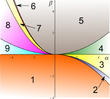
Figure 2: Phase space diagram in $(\alpha,\beta)$ for the solutions to the quintic equation (24) in $h$, where the different regions show different matching of inner solutions to asymptotic ones. The lines splitting the regions are half parabolas ($\beta\propto\alpha^{2}$, with $\alpha>0$ or $\alpha<0$) due to rescaling symmetry of eq. (24).

$\beta<0$
In this part of the phase space, there is only one inner solution, D, so there can be at most one global solution to (24). There are three distinct regions which differ in the way the matching works (see Koyama:Vainshtein for details):

• region 1: $\textbf{D}\leftrightarrow\textbf{C}_{+}$. The boundaries of this region are the line $\beta=0$ for $\alpha<0$ and the parabola $\beta=c_{12}\,\alpha^{2}$ for $\alpha>0$, where $c_{12}$ is the negative root of the equation $-4-8\,y+88\,y^{2}-1076\,y^{3}+2883\,y^{4}=0$.

• region 2: No matching. The boundaries of this region are the parabola $\beta=c_{12}\,\alpha^{2}$ and the parabola $\beta=c_{-}\,\alpha^{2}$, where $c_{-}$ is the only real root of the equation $8+48\,y-435\,y^{2}+676\,y^{3}=0$.

• region 3: $\textbf{D}\leftrightarrow\textbf{P}_{2}$.

$\beta>0$
In this part of the phase space, there are three inner solutions, D, $\textbf{F}_{+}$ and $\textbf{F}_{-}$, so there can be at most three global solutions to eq. (24). There are six distinct regions with different matching properties:

• region 4: $\textbf{F}_{-}\leftrightarrow\textbf{L}$ , $\textbf{D}\leftrightarrow\textbf{C}_{-}$. The boundaries of this region are the parabola $\beta=c_{45}\,\alpha^{2}$, where $c_{45}=1/12$, and the line $\beta=0$.

• region 5: $\textbf{F}_{+}\leftrightarrow\textbf{C}_{+}$ , $\textbf{F}_{-}\leftrightarrow\textbf{L}$, $\textbf{D}\leftrightarrow\textbf{C}_{-}$. The boundaries of this region are the parabola $\beta=c_{45}\,\alpha^{2}$ for $\alpha>0$ and the parabola $\beta=c_{56}\,\alpha^{2}$ for $\alpha<0$, where $c_{56}=(5+\sqrt{13})/24$.

• region 6: $\textbf{D}\leftrightarrow\textbf{C}_{-}$ , $\textbf{F}_{+}\leftrightarrow\textbf{C}_{+}$. The boundaries of this region are the parabolas $\beta=c_{56}\,\alpha^{2}$ and $\beta=c_{67}\,\alpha^{2}$, where $c_{67}$ is the positive root of the equation $-4-8\,y+88\,y^{2}-1076\,y^{3}+2883\,y^{4}=0$.

• region 7: $\textbf{F}_{+}\leftrightarrow\textbf{C}_{+}$. The boundaries of this region are the parabola $\beta=c_{67}\,\alpha^{2}$ and the parabola $\beta=c_{+}\,\alpha^{2}$, where $c_{+}=1/4$.

• region 8: $\textbf{F}_{+}\leftrightarrow\textbf{C}_{+}$ , $\textbf{F}_{-}\leftrightarrow\textbf{P}_{1}$ , $\textbf{D}\leftrightarrow\textbf{P}_{2}$. The boundaries of this region are the parabolas $\beta=c_{+}\,\alpha^{2}$ and $\beta=c_{89}\,\alpha^{2}$, where $c_{89}=(5-\sqrt{13})/24$.

• region 9: $\textbf{F}_{-}\leftrightarrow\textbf{P}_{1}$ , $\textbf{D}\leftrightarrow\textbf{P}_{2}$.

We note that the decaying solution L never connects to the diverging configuration D, so we can not have a spacetime which is asymptotically flat and exhibits the self-shielding of the gravitational field at the origin. On the other hand, finite non-zero asymptotic solutions ($\textbf{C}_{\pm}$ or $\textbf{P}_{1,2}$) can connect to both finite and diverging inner solutions. Therefore, one can have an asymptotically non-flat spacetime which presents self-shielding at the origin, or an asymptotically non-flat spacetime which tends to Schwarzschild spacetime for small radii. More precisely, for $\beta<0$ there are only solutions displaying the self-shielding of the gravitational field, apart from region 2 where there are no global solutions. Therefore the Vainshtein mechanism never works for $\beta<0$. In contrast, for $\beta>0$ all three kinds of global solutions are present. Solutions with asymptotic flatness and the Vainshtein mechanism are present in regions 4 and 5, while solutions which are asymptotically non-flat and exhibit the Vainshtein mechanism do exist in all ($\beta>0$) regions but region 4. Finally, solutions which display the self-shielding of the gravitational field are present in all ($\beta>0$) regions but region 7.

For the sake of clearness, we show one representative plot with the numerical matching solution between the inner and the asymptotic solutions. We consider solutions which recover the Schwarzschild solution near the origin, and which are asymptotically flat ($\textbf{F}_{-}\leftrightarrow\textbf{L}$ in Figure 3-left), or non-flat ($\textbf{F}_{+}\leftrightarrow\textbf{C}_{+}$ in Figure 3-right). Finally, it is essential to decide whether these vacuum solutions are indeed consistent with matter sources, as it was done for the $\beta=0$ case in Berezhiani:2013dw .

The Vainshtein mechanism has been studied intensively in the context of the Dvali-Gabadadze-Porrati braneworld model DGP and Galileon models Vainshtein . Especially, it was shown that the most general second order scalar tensor theory described by the Hordenski action Hordenski leads to the same field equations as massive gravity Narikawa .

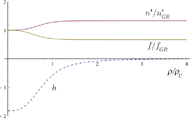
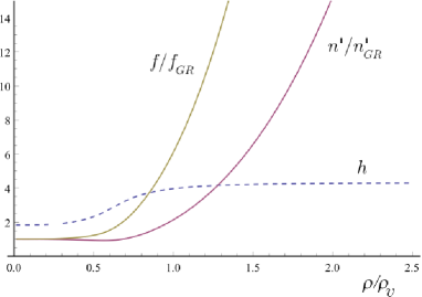
Figure 3: Numerical solutions for $\textbf{F}_{-}\leftrightarrow\textbf{L}$ (left) and $\textbf{F}_{+}\leftrightarrow\textbf{C}_{+}$ (right), with $(\alpha,\beta)=(0\,,0.1)$. $f_{GR}=n_{GR}=-2GM/\rho$. Solutions represent the GR gravitational potentials, and clearly present the vDVZ discontinuity with its resolution via the Vainshtein mechanism. Solutions asymptote a flat spacetime but with a different $\gamma=f/n$ than the Schwarzschild solution in GR (left) and a non-flat spacetime (right).

III.2 Branch II: exact solutions

As we learned in the previous section, an essential property of this theory of massive gravity is the strong coupling phenomenon occurring in the proximity of a source. On the other hand, the graviton mass induces non-linearities in the behavior of long wave length gravitons, responsible for the emergence of the second branch of solutions that we are going to study in this section. In an appropriate gauge, these solutions are asymptotically de Sitter or Anti-de Sitter, depending on the choice of parameters.

We start with the unitary gauge ($\pi^{\mu}=0$) and allow for arbitrary couplings $\alpha_{3}$ and $\alpha_{4}$, while from now on we set, for simplicity, the bare cosmological constant to vanish (see Koyama:prl ; Koyama:solutions for a more complete discussion including a bare cosmological constant). We choose the static Ansatz of eq. (12) for the metric, and we focus on the second branch of solutions for the constraint equation (13): $c(r)\,=\,c_{0}\,r$. Then, the exact solution of field equations is given by Salam ; Koyama:prl ; Koyama:solutions ,

$$c(r) = c_{0}\,r\,,$$

$$b(r)^{2} = b_{0}+\frac{b_{1}}{r}+b_{2}\,r^{2}\,,$$

$$a(r)^{2}+b(r)^{2} = Q_{0}\,,$$

$$d^{2}(r)+a(r)^{2}b(r)^{2} = \Delta_{0}\,.$$ (30)

Moreover, the equations of motion fix the constant parameters $b_{0},b_{2},c_{0},Q_{0}$, leaving the values of $b_{1}$, $\Delta_{0}$ free (although their sizes must be contained within certain intervals). Notice that in General Relativity, diffeomorphism invariance allows one to choose the function $c(r)$ to be $c(r)\,=\,r$, so that $c_{0}=1$. In this theory of massive gravity, after having fixed the gauge, this choice is no longer possible and the equations of motion determine $c_{0}$. One finds

$$c_{0}\,=\,\frac{1+6\alpha_{3}+12\alpha_{4}\pm\sqrt{1+3\alpha_{3}+9\alpha_{3}^{2}-12\alpha_{4}}}{3(1+3\alpha_{3}+4\alpha_{4})},$$ (31)

for non $\alpha_{3}\neq-4\alpha_{4}$, and

$$c_{0}=\frac{2}{3}\left(\frac{1-12\alpha_{4}}{1-8\alpha_{4}}\right),\\$$

for $\alpha_{3}=-4\alpha_{4}$, which in particular includes the case $\alpha_{3}=\alpha_{4}$=0. After plugging the metric components (30) in the remaining Einstein equations, one can find the values for the other parameters. The corresponding general expressions are quite lengthy, and for this reason we relegate them to Appendix A. As a concrete, simple example, in the main text we work out the special case $\alpha_{3}=-4\,\alpha_{4}$, where the parameters are

$${c_{0}}=\frac{2}{3}\left(\frac{1-12\alpha_{4}}{1-8\alpha_{4}}\right)\,,\qquad \qquad b_{0}=\frac{\Delta_{0}}{c_{0}^{2}},$$

$$b_{2}=\frac{m^{2}\,\Delta_{0}}{4\left(12\alpha_{4}-1\right)}\,,\qquad \qquad Q_{0}=\frac{16(1-12\alpha_{4})^{4}+81(1-8\alpha_{4})^{4}\Delta_{0}}{36\left[1+4\alpha_{4}(-5+24\alpha_{4})\right]^{2}}.$$ (32)

The previous solution is valid for $\alpha_{4}$ in the ranges $\alpha_{4}<1/12$ and $\alpha_{4}>1/8$. We find that $b_{1}$ and $\Delta_{0}$ are arbitrary; this vacuum solution is then characterized by two integration constants. The resulting metric coefficients can be rewritten in the following, easier-to-handle form:

$$a(r)^{2} = \frac{9}{4}\,\Delta_{0}\,\left(\frac{1-8\alpha_{4}}{1-12\alpha_{4}}\right)^{2}\,\left[p(r)+\gamma+1\right]\hskip 14.22636pt,\hskip 14.22636ptc(r)\,=\,\frac{2}{3}\,\left(\frac{1-12\alpha_{4}}{1-8\alpha_{4}}\right)\,r$$

$$b(r)^{2} = \frac{9}{4}\,\Delta_{0}\,\left(\frac{1-8\alpha_{4}}{1-12\alpha_{4}}\right)^{2}\,\left[1-p(r)\right]\hskip 14.22636pt,\hskip 14.22636pt$$ (33)

$$d(r) = \frac{9\Delta_{0}}{4}\,\left(\frac{1-8\alpha_{4}}{1-12\alpha_{4}}\right)^{2}\,\sqrt{p(r)\left(p(r)+\gamma\right)}$$

with ($\mu=-b_{1}/b_{0}$)

$$p(r)\,\equiv\,\frac{\mu}{r}+\frac{\left(1-12\alpha_{4}\right)\,m^{2}\,r^{2}}{9\,(1-8\alpha_{4})^{2}}\,\hskip 22.76228pt,\hskip 22.76228pt\gamma\,\equiv\,\frac{16}{81\Delta_{0}}\,\left(\frac{1-12\alpha_{4}}{1-8\alpha_{4}}\right)^{4}-1\,.$$ (34)

In order to have a consistent solution, we must demand that the argument of the square root appearing in the expression for $d(r)$, Eq. (33), is positive. A sufficient condition to ensure this is that $\mu\geq 0$, and

$$0\,<\,\sqrt{\Delta_{0}}\,<\,\frac{4}{9}\,\left(\frac{1-12\alpha_{4}}{1-8\alpha_{4}}\right)^{2}\,.$$ (35)

The metric might be rewritten in a more transparent diagonal form, by means of a coordinate transformation. In absence of diffeomorphism invariance, any coordinate transformation of time $t$ forces us to leave the unitary gauge, and to switch on a non-trivial profile for the Stückelberg field $\pi^{\mu}$ of the form $\pi^{\mu}\,=\,\left(\pi_{0}(r),0,0,0\right)$. One finds that then the metric can be rewritten in a diagonal form, as

$$ds^{2}\,=\,-b(r)^{2}dt^{2}+\tilde{a}(r)^{2}dr^{2}+c(r)^{2}\,d\Omega^{2},$$ (36)

while the equations of motion for the fields involved are solved by

$$\tilde{a}(r)^{2}\,=\,\frac{4}{9}\,\left(\frac{1-12\alpha_{4}}{1-8\alpha_{4}}\right)^{2}\frac{1}{1-p(r)}\hskip 22.76228pt,\hskip 22.76228pt\pi_{0}^{\prime}(r)\,=\,-\frac{\sqrt{p(r)(p(r)+\gamma)}}{1-p(r)},$$ (37)

with $b(r)$, $c(r)$ and $p(r)$ being the same as in Eq. (33). If one then makes a further time rescaling

$$t\to\frac{4\left(1-12\alpha_{4}\right)^{2}}{9\Delta_{0}^{1/2}\left(1-8\alpha_{4}\right)^{2}}\,t\;,$$ (38)

the resulting metric acquires a manifestly de Sitter-Schwarzschild, or Anti-de Sitter-Schwarzschild form. The choice between these two possibilities depends on whether $\alpha_{4}$ is smaller or larger than $1/12$, as can be seen inspecting the function $p(r)$ in Eq. (34). On the other hand, we should point out that this time-rescaling cannot be performed, without further introducing a time dependent contribution to $\pi_{0}$. As expected, the metric in Eq. (36) can also be obtained by making the following transformation of the time coordinate $d\tilde{t}\,=\,dt+\pi_{0}^{\prime}dr$ to the original metric (12). This produces a non-zero time component for $\pi^{\mu}$, that does not vanish even in the limit $m\to 0$.

To summarize so far, we found vacuum solutions in this theory that are asymptotically de Sitter or Anti-de Sitter, depending on the choice of the parameters.

Figure 4 shows the allowed parameters $\alpha_{3}$ and $\alpha_{4}$ for the existence of these asymptotically dS or AdS solutions. Further solutions and studies on black holes in this massive gravity theory can be found in sbh .

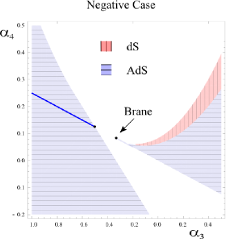
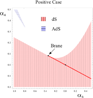
Figure 4: Allowed region of parameter space where solutions, which asymptote dS (vertical lines in light or red color) or AdS (horizontal lines in dark or blue color), exist. Left (right) plot is for the negative (positive) branch of Eq. (31). The brane solution is given by the special choice of for $\alpha_{3}=-1/3$ and $\alpha_{4}=1/12$ Koyama:solutions , and the solid lines correspond to the line $\alpha_{3}=-4\alpha_{4}$. We have set $\Lambda=0$.

IV Cosmological Acceleration

IV.1 Self-accelerating solution

One of the interesting features of massive gravity is self-acceleration. The self-accelerating solution was originally found in the DGP braneworld model where the acceleration of the Universe can be realised without introducing the cosmological constant DGPcosmo . However the self-accelerating solution in the DGP model suffers from a ghost instability DGPghost .

The first complete self-accelerating solution in the $\Lambda_{3}$ massive gravity theory (6) was reported in Koyama:solutions ; Koyama:prl (the self-accelerating solution in the decoupling limit was first obtained in deRham:2010tw ). This configuration describes an accelerating cosmological universe in the vacuum, in which the rate of acceleration is controlled by the size of the graviton mass. The solution is a coordinate transformation of the exact solution (36)-(37), after having performed the time rescaling (38) (one can use (76)-(78) for more general values of $\alpha_{3}$ and $\alpha_{4}$). Let us review how to construct it for the simple case of $\alpha_{3}=-4\alpha_{4}$. In the case of the asymptotically de Sitter solution (36)-(37) with $\alpha_{4}<1/12$ and $\mu=0$, the metric can also be written in a time dependent form, at the price of switching on additional components of $\pi^{\mu}$. After dubbing

$$\tilde{m}^{2}\equiv\frac{m^{2}}{(1-12\alpha_{4})}$$

we can make the following coordinate transformation $t\,=\,F_{t}(\tau,\rho)$ and $r\,=\,F_{t}(\tau,\rho)$ with

$$F_{t}(\tau,\rho) = \frac{4}{3\,\Delta_{0}^{1/2}\,\tilde{m}}\,\Big{(}\frac{1-12\alpha_{4}}{1-8\alpha_{4}}\Big{)}\,{\rm arctanh}\,\left(\frac{\sinh{\left(\frac{\tilde{m}\tau}{2}\right)}+\frac{\tilde{m}^{2}\rho^{2}}{8}e^{\tilde{m}\tau/2}}{\cosh{\left(\frac{\tilde{m}\tau}{2}\right)}-\frac{\tilde{m}^{2}\rho^{2}}{8}e^{\tilde{m}\tau/2}}\right),$$ (39)

$$F_{r}(\tau,\rho) = \frac{3}{2}\Big{(}\frac{1-8\alpha_{4}}{1-12\alpha_{4}}\Big{)}\rho\,e^{\tilde{m}\tau/2}.$$ (40)

Then, the metric becomes that of flat slicing of de Sitter

$$ds^{2}\,=\,-d\tau^{2}+e^{{\tilde{m}}\tau}\,\left(d\rho^{2}+\rho^{2}d\Omega^{2}\right),$$ (41)

where the Hubble parameter is given by

$$H\,=\,\frac{\tilde{m}}{2}\,=\,\frac{m}{2(1-12\alpha_{4})^{\frac{1}{2}}}$$ (42)

The Stückelberg fields $\pi^{\mu}$ are now given by

$$\pi^{\mu}\,=\,\left(\,\pi_{0}+\tau-F_{t},\,\rho-\,F_{r},\,0,\,0\right).\$$ (43)

Interestingly, the value of the Hubble parameter is ruled by the mass of the graviton: we have a self-accelerating solution, in which the smallness of the acceleration rate can be associated with the smallness of the graviton mass.

So far, we used the general static solutions of the previous section to determine time-dependent self-accelerating configurations via suitable coordinate transformations. However, one can also follow another approach, and try to directly find time-dependent, self-accelerating configurations in the theory of $\Lambda_{3}$ massive gravity without relying on the unitary gauge. The hope, following this second route, is to determine additional cosmological configurations for this theory. Starting from the Ansatz we wrote in eq. (10), more general cosmological solutions can be obtained by focussing on the Ansatz $d(r,t)=0$ and $c(r,t)\,=\,r\,a(r,t)$ in (10) so that the metric becomes

$$ds^{2}=-b(t,r)^{2}dt^{2}+a(t,r)^{2}(dr^{2}+r^{2}d\Omega^{2}).$$ (44)

Wyman et al wyman showed that self-accelerating configurations are characterised by the following profile for the function $g(r,t)$ characterizing the Stückelberg field $\phi^{i}$ (see eq (11))

$$g(t,r)=c_{0}^{-1}a(t,r)r,$$ (45)

where $c_{0}$ is given by (31). The equation of motion for $g$ evaluated on the solution (45) provides a constraint on the function $f$ characterizing the Struckelberg field $\phi^{0}$

$$\sqrt{{X}}P_{1}^{\prime}=\left(2c_{0}P_{2}-P_{2}^{\prime}\right)W-P_{0}^{\prime},$$ (46)

where the $P_{n}$ functions

$$P_{0}(x) = -12-2x(x-6)-12(x-1)(x-2)\alpha_{3}-24(x-1)^{2}\alpha_{4},$$

$$P_{1}(x) = 2(3-2x)+6(x-1)(x-3)\alpha_{3}+24(x-1)^{2}\alpha_{4},$$

$$P_{2}(x) = -2+12(x-1)\alpha_{3}-24(x-1)^{2}\alpha_{4}.$$ (47)

are evaluated at $x=c_{0}^{-1}$, $P_{n}^{\prime}(x)\equiv dP_{n}/dx$. Moreover,

$${X}=\Bigl{(}\frac{\dot{f}}{b}+\mu\frac{g^{\prime}}{{a}}\Bigr{)}^{2}-\Bigl{(}\frac{\dot{g}}{b}+\mu\frac{f^{\prime}}{{a}}\Bigr{)}^{2},\quad W=\frac{\mu}{ab}(\dot{f}g^{\prime}-\dot{g}f^{\prime}),$$ (48)

and $\mu={\rm sgn}(\dot{f}g^{\prime}-\dot{g}f^{\prime})$ where primes denote derivatives with respect to $r$ and overdots with respect to $t$. Using these equations, it is possible to show that the Einstein equations are given by

$$G^{\mu}_{\nu}=-3H^{2}\delta^{\mu}_{\nu},\quad H^{2}=\frac{1+3\alpha_{3}\pm 2\alpha_{5}}{3(1+3\alpha_{3}\pm\alpha_{5})^{2}}m^{2},$$ (49)

where

$$\alpha_{5}^{2}\equiv 1+3\alpha_{3}+9\alpha_{3}^{2}-12\alpha_{4}\,.$$ (50)

Note that there are two branches of solutions. This approach leads to self-accelerating solutions where the Hubble parameter is determined by the mass of the graviton.

There are many possible solutions for the function $f(t,r)$ for given solutions of metric satisfying the Einstein equations (49). For example, in the simple case of $\alpha_{3}=\alpha_{4}=0$, the configuration (41) and (43) is given by

$$b=1,\quad a=e^{mt/2},\quad f(t,r)=-\frac{3}{2}e^{mt/2}r+\frac{3}{m}\left({\rm arctanh}\left(\frac{1}{2}e^{mt/2}mr\right)+{\rm arctanh}\left(\frac{4-e^{mt}(4+m^{2}r^{2})}{-4+e^{mt}(-4+m^{2}r^{2})}\right)\right).$$ (51)

Notice that this self-accelerating solution has a flat FRWL metric, however, one can also write it as an open or closed FRWL spacetime, with the price of changing the Stückelberg fields accordingly. In all the FRWL frames, the Stückelberg fields are inhomogeneous. In fact it was suggested that there was no FRW solution that keeps the FRW symmetry for the fiducial metric $\Sigma^{\mu}_{\nu}$ D'Amico:2011jj . However, Gumrukcuoglu et al found a special self-accelerating solution which represents an open universe where the fiducial metric $\Sigma_{\mu\nu}$ respects the FRW symmetries of the physical metric $g_{\mu\nu}$ Gumrukcuoglu:2011ew . Their solution is given by

$$b=1,\quad a=\frac{a_{0}(t)}{1-(mr)^{2}/16},\quad f(t,r)=\frac{3}{m}a_{0}(t)\frac{1+(mr)^{2}/16}{1-(mr)^{2}/16},\quad a_{0}(t)=\sinh(mt/2).$$ (52)

For this solution the fiducial metric preserves the FRW symmetry, $\Sigma^{\mu}_{\nu}=(9/4){\rm diag}((2\dot{a}_{0}/m)^{2},1,1,1)$. The behaviour of perturbations around this particular self-accelerating solution is very different from the other solutions that break the FRW symmetry for the fiducial metric $\Sigma^{\mu}_{\nu}$. At the linear order, scalar and vector perturbations have no kinetic terms, hence they are strongly coupled Gumrukcuoglu:2011zh , which leads to non-linear instabilities DeFelice:2012mx ; DeFelice:2013awa . The absence of the scalar kinetic term originates from the special choice of the solution for $f$ Wyman2 that retains the FRW symmetry for the fiducial metric. This leads to an enhanced symmetry that eliminates the scalar perturbations new . In the rest of this review, we do not consider this class of self-accelerating solution and consider the case where the FRW symmetry is broken for the fiducial metric $\Sigma^{\mu}_{\nu}$. However, we emphasise that the physical metric still retains the FRW symmetry in these solutions.

Wyman et al wyman also showed that the ordinary Friedmann equation is obtained even if we add ordinary matter energy density $\rho_{m}(t)$. The matter only sees the effect of the mass terms as a cosmological constant with no direct coupling to the scalar fields on the exact solution. Cosmological solutions in massive gravity and its extension including de a Sitter fiducial metric and bigravity can be found in cosmorefs .

IV.2 Decoupling limit solutions and their instability

Once we determined self-accelerating, de Sitter solutions in this model, it is crucial to study their stability: this is the subject of this section. In order to make the analysis manageable, we focus on a convenient limit of Lagrangian (6) which captures most of the dynamics of the helicity-0 and helicity-1 mode, but keeps the linear behaviour of the helicity-2 (tensor) mode ArkaniHamed:2002sp . The limit, called the decoupling limit, is defined as

$$m\to 0\,,\hskip 28.45274ptM_{Pl}\to\infty\,,\hskip 28.45274pt\Lambda_{3}\,\equiv\,m^{2}M_{Pl}=\,{\text{fixed}}\,,$$ (53)

In order to obtain canonically normalized kinetic terms for the helicity 2 and helicity 1 modes, together with the relevant couplings for the helicity 0 modes, when this limit is taken one needs to canonically normalise the fields in the following way

$$h_{\mu\nu}\,\to\,M_{Pl}\,h_{\mu\nu}\,,\hskip 14.22636ptA_{\mu}\,\to\,mM_{Pl}\,A_{\mu}\,,\hskip 14.22636pt\pi\,\to\,m^{2}M_{Pl}\,\pi,$$ (54)

where we have split the Stückelberg fields $\pi^{\mu}$ into a scalar component $\pi$ and a divergenceless vector $A^{\mu}$ in the usual way, namely

$$\pi^{\mu}=\eta^{\mu\nu}(\partial_{\nu}\pi+A_{\nu}).$$ (55)

In order to take the decoupling limit (53) of the self-accelerating solutions defined by (45), the solution has to be in the conformally flat frame, which is defined as follows

$$a(t,r)=b(t,r)=\frac{c(t,r)}{r}=(1+H^{2}(r^{2}-t^{2})/4)^{-1}.$$ (56)

In this frame, all the known self-accelerating solutions lead to the same decoupling limit solution for the Stückelberg fields, namely

$$\pi^{0} = \left(\frac{1+3\alpha_{3}+\alpha_{5}}{(2+3\alpha_{3}+\alpha_{5})\sqrt{\Delta_{0}}}-1\right)t-\frac{1}{2}\sqrt{\frac{(1+3\alpha_{3}+2\alpha_{5})\left[(1+3\alpha_{3}+\alpha_{5})^{4}-(2+3\alpha_{3}+\alpha_{5})^{4}\Delta_{0}\right]}{3\Delta_{0}(1+3\alpha_{3}+\alpha_{5})^{4}(2+3\alpha_{3}+\alpha_{5})^{2}}}mr^{2}+\mathcal{O}(m^{2})$$

$$\pi^{r} = -\frac{1}{1+3\alpha_{3}+\alpha_{5}}r+\mathcal{O}(m^{2}),$$ (57)

with $\alpha_{5}$ given by eq. (50). If we split $\pi^{\mu}$ into a scalar and vector piece as in (55), canonically normalise the fields as in (54), and take the decoupling limit (53), one gets Koyama:vect1 ; Koyama:vect2

$$h_{\mu\nu} = -\frac{1}{2}\Lambda_{3}H^{2}(r^{2}-t^{2})\eta_{\mu\nu},$$

$$\pi = -\frac{1}{2}\left(1-\frac{1}{c_{0}}\sqrt{1+\frac{3(1+3\alpha_{3}+\alpha_{5})^{4}Q_{0}^{2}}{(2+3\alpha_{3}+\alpha_{5})^{2}(1+3\alpha_{3}+2\alpha_{5})}}\right)\Lambda_{3}t^{2}-\frac{c_{0}-1}{2\,c_{0}}\Lambda_{3}r^{2},$$

$$A_{0} = -\frac{Q_{0}}{2}\Lambda_{3}r^{2},$$ (58)

where $c_{0}$ is given by (31) (or (III.2) for $\alpha_{3}=-4\alpha_{4}$), and the Hubble parameter $H$ by

$$H^{2}=\frac{(1+3\alpha_{3}\pm 2\alpha_{5})m^{2}}{3(1+3\alpha_{3}\pm\alpha_{5})^{2}},$$ (59)

which is the generalisation of (42) for arbitrary $\alpha_{3}$ and $\alpha_{4}$. Moreover, there is a relation between $\Delta_{0}$ and $Q_{0}$

$$\Delta_{0}=\frac{(1+3\alpha_{3}+\alpha_{5})^{4}(1+3\alpha_{3}+2\alpha_{5})}{3Q_{0}^{2}(2+3\alpha_{3}+\alpha_{5})^{2}(1+3\alpha_{3}+\alpha_{5})^{4}+(2+3\alpha_{3}+\alpha_{5})^{4}(1+3\alpha_{3}+2\alpha_{5})},$$ (60)

and in the case of AdS, there is an extra bound given by

$$Q_{0}^{2}<\frac{(2+3\alpha_{3}+\alpha_{5})^{2}(1+3\alpha_{3}+2\alpha_{5})}{3(1+3\alpha_{3}+\alpha_{5})^{4}}.$$ (61)

If one take the vector charge to zero $Q_{0}=0$ (or equivalently if $\Delta_{0}=(1+3\alpha_{3}+\alpha_{5})^{4}/(2+3\alpha_{3}+\alpha_{5})^{4}$), these solutions can be written in a simpler covariant way

$$h_{\mu\nu}=-\frac{1}{2}\Lambda_{3}H^{2}(x^{\mu}x_{\mu})\eta_{\mu\nu}\qquad\qquad\pi=\frac{c_{0}-1}{2\,c_{0}}\Lambda_{3}x^{\mu}x_{\mu},\qquad\qquad A^{\mu}=0.$$ (62)

Therefore, corrections of order $m^{2}$ in (IV.2), which do not show in the decoupling limit, are the main differences among solutions in the full theory. These solutions in the decoupling theory were also found in deRham:2010tw .

In this decoupling limit, the structure of the Lagrangian becomes much simpler, and the various self-accelerating configurations become the same. For these reasons, it is particularly convenient to study the dynamics of perturbations in this limit. If problems or instabilities arise in this limit, then are they unavoidably present also in the full theory outside the decoupling regime. Interestingly, it has been shown in deRham:2010tw that, in the decoupling limit, the coupling between the scalar mode $\pi$ and the trace $T$ of the energy momentum tensor vanishes around these self-accelerating configurations: hence, the coupling to matter is the same as in GR with no need to implement a Vainshtein mechanism. However, we have shown in Koyama:vect1 ; Koyama:vect2 that all these backgrounds present instabilities in the vector sector. We present here the main results concerning these instabilities, focussing on the case of $\alpha_{3}=\alpha_{4}=0$. A generalisation to arbitrary values is straighforward and can be found in Koyama:vect1 ; Koyama:vect2 . We start by considering perturbations of the fields $h_{\mu\nu}$, $A^{\mu}$ and $\pi$ which only depend on time and radial component. Namely

$$h_{\mu\nu}=h^{0}_{\mu\nu}+\hat{h}_{\mu\nu},\qquad\qquad A^{\mu}=A^{\mu}_{0}+\hat{A}^{\mu},\qquad\qquad\pi=\pi_{0}+\hat{\pi},$$ (63)

where the background quantities (those with an index $0$) are given by the self-accelerating solution (62). The Lagrangian for the tensor and scalar perturbations (without further truncations) reads

$${\cal L}_{h_{\mu\nu},\;\pi} = -\frac{1}{2}\,\hat{h}^{\mu\nu}{\cal E}_{\mu\nu}^{\alpha\beta}\hat{h}_{\alpha\beta}+\hat{h}^{\mu\nu}{X}_{\mu\nu}-6H^{2}\,\hat{\pi}\Box\hat{\pi}\,,$$ (64)

where (in units in which $\Lambda_{3}=1$, that we adopt from now on) $H^{2}=\frac{1}{4}$ and $\hat{X}_{\mu\nu}$ is given by

$$\hat{X}_{\mu\nu} = \Big{[}\hat{\Pi}_{\mu}^{\lambda}\hat{\Pi}_{\lambda\nu}-\hat{\Pi}\hat{\Pi}_{\mu\nu}+\frac{1}{2}\eta_{\mu\nu}\left(\hat{\Pi}^{2}-\hat{\Pi}_{\mu}^{\nu}\hat{\Pi}_{\nu}^{\mu}\right)\Big{]}\,.$$ (65)

We can use the following field redefinition to decouple the helicity 2 from the helicity 0 field:

$$\hat{h}_{\mu\nu}\,\to\,\hat{h}_{\mu\nu}-\partial_{\mu}\hat{\pi}\partial_{\nu}\hat{\pi}\,.$$ (66)

Then the kinetic terms for tensor and scalar are diagonalized resulting, up to total derivatives, in

$${\cal L}_{h_{\mu\nu},\;\pi} = -\frac{1}{2}\hat{h}_{\mu\nu}{\cal E}^{\mu\nu\alpha\beta}\hat{h}_{\alpha\beta}-6H^{2}\hat{\pi}\Box\hat{\pi}-\frac{1}{2}\left(\partial\hat{\pi}\right)^{2}\left[\left(\Box\hat{\pi}\right)^{2}-\left(\partial_{\mu}\partial_{\nu}\hat{\pi}\partial^{\mu}\partial^{\nu}\hat{\pi}\right)\right]\,.$$ (67)

Let us emphasize that the previous Lagrangian contains terms which are quadratic on $\hat{h}_{\mu\nu}$, but higher orders in the scalar field $\hat{\pi}$. The scalar field terms are the so called Galileon combinations. On the contrary, as mentioned before, the vector piece has an infinite number of interactions Koyama:vect1 ; Koyama:vect2 . For our purposes, it is enough to stop at fourth order in the fields, resulting in the Lagrangian

$${\cal L}_{A_{\mu}} = \frac{1}{18}\Big{\{}3\hat{\Pi}\,F^{\mu\nu}F_{\mu\nu}-6\,\left(\hat{\Pi}^{\alpha}_{\ \mu}F^{\mu\nu}F_{\nu\alpha}\right)$$ (68)

$$-2\left[\hat{\Pi}^{\mu}_{\ \nu}\hat{\Pi}^{\nu}_{\ \alpha}F^{\alpha\beta}F_{\beta\mu}+\hat{\Pi}^{\mu}_{\ \nu}F^{\nu\alpha}\hat{\Pi}^{\ \beta}_{\alpha}F_{\beta\mu}-\hat{\Pi}\,(\hat{\Pi}^{\alpha}_{\ \mu}F^{\mu\nu}F_{\nu\alpha})\right]\Big{\}}\,+\,\dots$$

where $F_{\mu\nu}=\partial_{\mu}A_{\nu}-\partial_{\nu}A_{\mu}$. As mentioned above, the kinetic terms for the vectors vanish; however, vectors become dynamical by coupling them with the scalar at third or higher order in fluctuations (this was already pointed out in deRham:2010tw ; Koyama:vect1 ; D'Amico:2012pi ). Nevertheless, one should worry about higher derivatives in the equations of motion, since the previous Lagrangian contains contributions with two time derivatives in the scalar field $\pi$. For systems coupling scalars with vectors, it is possible to find the combination that ensures that the equations of motion do not contain at all terms containing more than two time derivatives. It is a generalization of Galileon combinations which was explored in Deffayet:2010zh and dubbed $p$-form Galileons. Up to fourth order in perturbations, the correct combination (without including higher derivatives in $A_{\mu}$) is

$${\cal L}^{p-form}\,=\,a_{0}\,\left[{\rm tr}\Pi\,{\rm tr}F^{2}-2\,{\rm tr}\Pi F^{2}\right]+b_{0}\,\left\{{\rm tr}F^{2}\,\left[{\rm tr}\Pi^{2}-\left({\rm tr}\Pi\right)^{2}\right]-4{\rm tr}\Pi\,{\rm tr}\Pi F^{2}+4{\rm tr}\Pi^{2}F^{2}+2{\rm tr}\Pi F\Pi F\right\}$$ (69)

where $a_{0}$ and $b_{0}$ are arbitrary coefficients, and we have used the ${\rm tr}$ notation to simplify the index structure. The above third order action with the aforementioned properties was presented in Deffayet:2010zh , while the fourth order one is as far as we know new. Comparing (68) with (69) we notice that while the third order action has the correct structure to avoid higher order time derivatives in the equation of motion, the fourth order Lagrangian does not seem to satisfy this requirement. However, a suitable field redefinition allows to remove the fourth order term from the third order contribution, leaving a healthy Lagrangian without higher derivative equations of motion (in agreement with the ghost-free statement of the theory).

On the other hand, although our scalar-vector Lagrangian (68) does not lead to a propagation of a sixth ghost mode, it does generally lead to a ghost-like instability around self-accelerating configurations, in which the ghost is one of the available vector modes. It has be shown in Koyama:vect1 that, when turning on a non-trivial profile for the background vector field, the corresponding Lagrangian for perturbations around the resulting configuration acquires kinetic terms for the vector with the wrong sign. Here, following Koyama:vect2 , we instead directly point out the instability by analyzing the Hamiltonian associated with the Lagrangian obtained by combining the third order Lagrangian contained in (68) with the scalar kinetic term:

$${\cal L}^{third}\,=\,-3H^{2}{\pi}\Box{\pi}-\frac{1}{6}\left[\Box\pi\,F_{\mu\nu}F^{\mu\nu}-2\partial_{\mu\nu}\pi F^{\mu\rho}F^{\nu}_{\;\;\rho}\right],$$ (70)

where we have removed the hats over the field to simplify the notation. We choose, for simplicity, the gauge $A_{0}=0$, $\partial_{i}A_{i}=0$, and by doing a standard $(3+1)$-decomposition, the previous Lagrangian reads

$${\cal L}\,=\,-3H^{2}\dot{\pi}^{2}+\frac{1}{3}\,\left[2\dot{\pi}\,\dot{A}_{i}\triangle A_{i}+\triangle\pi\,\dot{A}_{i}^{2}-\pi_{,\,ij}\,\dot{A}_{i}\dot{A}_{j}\right]+\dots$$ (71)

where the dots represent the terms without time derivatives, which we do not include since they do not play a role in the present discussion. The conjugate momenta to $\pi$ and $A_{i}$ are

$$\Pi_{\pi}=-6H^{2}\,\left(\dot{\pi}-\frac{1}{9\,H^{2}}\,\dot{A}_{i}\triangle A_{i}\right)\,,\qquad\qquad\Pi_{A_{i}}=\frac{2}{3}\left[\dot{\pi}\,\triangle A_{i}+\triangle\pi\,\dot{A}_{i}-\pi_{,\,ij}\,\dot{A}_{j}\right]\,.$$ (72)

In order to analyze the associated Hamiltonian, it is convenient to introduce the matrix ${\kappa}_{ij}\,\equiv\,\triangle\pi\,\delta_{ij}-\pi_{,\,ij}$. If $\kappa_{ij}\,=\,0$, then, we can easily invert the relations that define the conjugate momenta, and obtain the following Hamiltonian

$${\cal H} = -\frac{\Pi_{\pi}^{2}}{12\,H^{2}}+\frac{1}{12H^{2}}\,\left(\Pi_{\pi}+\frac{9\,H^{2}\,A_{i}\Pi_{A_{i}}}{A_{i}\,\triangle A_{i}}\right)^{2}+\dots\,,$$ (73)

$$= \frac{3}{2}\,\Pi_{\pi}\,\frac{A_{i}\Pi_{A_{i}}}{A_{i}\,\triangle A_{i}}+\frac{27\,H^{2}}{4}\,\left(\frac{A_{i}\Pi_{A_{i}}}{A_{i}\,\triangle A_{i}}\right)^{2}+\dots\,,$$ (74)

where the dots represent terms without momentum variables. The previous Hamiltonian is linear in $\Pi_{\pi}$; hence it is unbounded from below. Notice that this argument holds even in the limit in which $H^{2}$ vanishes. In conclusion, perturbations of the background self-accelerating solution, along the direction of scalar fluctuations such that ${\kappa}_{ij}\,=\,0$, admit unstable directions along which the system falls towards regions where the energy is unbounded from below. Similar conclusions hold for more generic $\kappa_{ij}$. Let us, for example, consider a $\kappa_{ij}$ that is non-vanishing, and invertible. Then, after straightforward manipulations, one can show that the Hamiltonian can be written as

$$\frac{4}{3}\,{\cal H}\,=\,-\frac{1}{9H^{2}+\Delta A_{i}\kappa_{ij}^{-1}\Delta A_{j}}\,\left(\Pi_{\pi}-\Delta A_{i}\kappa_{ij}^{-1}\Pi_{A_{j}}\right)^{2}+\Pi_{A_{i}}\kappa_{ij}^{-1}\Pi_{A_{j}}+\dots\,,$$ (75)

where, again, the dots represent terms without momentum variables. It is not difficult to see that there are many unstable directions associated with this Hamiltonian. For example, make a choice for the vector $\Delta A_{i}$ so that the scalar combination ${\cal C}\,\equiv\,\Delta A_{i}\kappa_{ij}^{-1}\Delta A_{j}$ is non-vanishing and has a given sign. For definiteness, the magnitude of $\Delta A_{i}$ is chosen such that the denominator of the first term has the same sign of ${\cal C}$. Accordingly, choose the vector $\Pi_{A_{i}}$ such that $\Pi_{A_{i}}\kappa_{ij}^{-1}\Pi_{A_{j}}$ has the same sign of ${\cal C}$ (for example, choose it in the same direction of the $\Delta A_{i}$). Then, by choosing a suitable magnitude for $\Pi_{\pi}$, it is possible to make one of the two terms in the previous Hamiltonian arbitrarily negative – hence the Hamiltonian is unbounded from below. Other cases, such as the case in which $\kappa_{ij}^{-1}$ is non-vanishing but not invertible, can be treated in a similar way. Furthermore, while here we focussed on the case $\alpha_{3}=\alpha_{4}=0$ it is straightforward to extend this analysis to the more general case, obtaining the same conclusion (see Koyama:vect2 for details).

To summarize, one generically expects instabilities around the self-accelerating solutions discussed so far: there are many directions in the moduli space of fluctuations along which the energy is unbounded from below, and towards which the system can be driven into dangerous regions. On the other hand, to close this section with a positive perspective, it might very well be that suitable deformations of known solutions (or even completely new configurations) exist that, renouncing to the symmetries imposed on the Ansätze considered so far, do not present the problems discussed above. Very recently, a proposal in this direction has been pushed forward in DeFelice:2013awa , that consider the possibility of breaking the isotropy of three dimensional spatial slices to find stable configurations. Still much work is needed to clarify this subject and analyze phenomenological consequences of these solutions.

V Future directions

Massive gravity is a good theoretical laboratory to study modifications of General Relativity with interesting phenomenological consequences. Non-linear self-interactions of massive gravity in proximity of a source manage to mimic the predictions of linearised General Relativity, hence agreeing with solar-system precision measurements. Moreover, massive gravity offers a concrete set-up for studying models of dark energy in modified gravity scenarios. Indeed, at large distances gravity is modified with respect to GR, and the theory admits cosmological accelerating solutions in the vacuum in which the size of acceleration depends on the graviton mass. Dark energy models built in this way have the opportunity to be technically natural in the ’t Hooft sense: in the limit of graviton mass going to zero one gains a symmetry, by recovering the full diffeomorphism invariance of GR. Consequently, any corrections to the size of dark energy must be proportional to the (tiny) graviton mass itself.

Hence, non-linear effects play a crucial role for characterizing phenomenological consequences of massive gravity. Motivated by this fact, the analysis of exact solutions of the equations of motion, obtained by imposing appropriate symmetries (spherical symmetry for static space-times, or homogeneity and isotropy for cosmological set-ups), make manifest, in idealized but representative situations, how the non-linear dynamics of the graviton degrees of freedom respond to the presence of a source, or, at very large scales, to the graviton mass itself. This has been the argument of this article, in which we reviewed our works on these topics.

Much interesting work is left for the future: our results can be extended in various directions that will improve our understanding of massive gravity and, in general, of consistent infrared modifications of General Relativity. From one side, it would be interesting to find new stationary configurations renouncing to spherical symmetry, to test analytically the effectiveness of Vainshtein mechanism when spherical symmetry is broken. As a concrete example, it would be interesting to find analogues of the Kerr geometry in this scenario, in which frame dragging effects can be quantitatively analyzed. Also, it would be interesting to determine cosmological configurations that break the isotropy or homogeneity of the cosmological solutions analyzed until now. Indeed, working in a suitable decoupling limit, we have shown that the cosmological self-accelerating configurations studied so far are characterized by instabilities in the vector sector. Given the recent results of DeFelice:2013awa , we speculate that these instabilities can be possibly avoided by renouncing to some of the symmetries that characterize the solutions (for example isotropy of the three spatial directions). It would be interesting to determine stable self-accelerating backgrounds following this route, and study their consequences for what respect the dynamics of cosmological fluctuations. We hope to be able to develp all these questions in our future work.

Appendix A General exact solution

From the general Lagrangian (6), and using the non-diagonal ansatz (12) together with Einstein equations (7), one can show that there are two branches of solutions for non-vanishing $\alpha_{3}$ and $\alpha_{4}$ as it was done in Section III. Here we only consider the branch with a non-diagonal metric, where analytic solutions can be found. Since the combination $\sqrt{1+3\alpha_{3}+9\alpha_{3}^{2}-12\alpha_{4}}$ is always present in the solution of this branch (see (31)), it is convenient to map the ($\alpha_{3},\alpha_{4}$) parameters into ($\alpha_{3},\alpha_{5}$), where $\alpha_{5}^{2}\equiv 1+3\alpha_{3}+9\alpha_{3}^{2}-12\alpha_{4}$. In this new set of parameters, the combination $d(r)\,G_{tt}+b(r)^{2}\,G_{tr}\,=\,0$, fixes $c(r)$ as a function of $r$ in the following way

$$c(r)=c_{0}r\,=\,\frac{(1+3\alpha_{3}+\alpha_{5})}{(2+3\alpha_{3}+\alpha_{5})}r.$$ (76)

The rest of Einstein equations give

$$b(r)^{2}=\frac{\Delta_{0}}{c_{0}^{2}}(1-p),\qquad a(r)^{2}=\frac{\Delta_{0}}{c_{0}^{2}}(p+\gamma+1),\qquad d(r)=\sqrt{\Delta_{0}-a(r)^{2}b(r)^{2}},$$ (77)

where

$$p=\frac{\mu}{r}+\frac{(1+3\alpha_{3}+2\alpha_{5})}{3(2+3\alpha_{3}+\alpha_{5})^{2}}m^{2}r^{2},\qquad\gamma+1=\frac{(1+3\alpha_{3}+\alpha_{5})^{4}}{\Delta_{0}(2+3\alpha_{3}+\alpha_{5})^{4}}$$ (78)

Just like in the $\alpha_{3}=\alpha_{4}=0$ ($\alpha_{5}=1$) case, there are two integration constants, $\mu$ and $\Delta_{0}$, but in order to have a positive argument for the square root in $d(r)$, $\Delta_{0}$ has to run from $\Delta_{0}=0$ to $\Delta_{0}^{max}=c_{0}^{2}$. If we focus on the massless case $\mu=0$ only, the solution describes the static patch of the de Sitter or Anti-de Sitter spacetime.

References

- (1) M. Fierz, W. Pauli, Proc. Roy. Soc. Lond. A173, 211-232 (1939).
- (2) D. G. Boulware, S. Deser, Phys. Rev. D6, 3368-3382 (1972).
- (3) N. Arkani-Hamed, H. Georgi, M. D. Schwartz, Annals Phys. 305, 96-118 (2003). [hep-th/0210184].
- (4) H. van Dam, M. J. G. Veltman, Nucl. Phys. B22, 397-411 (1970).
- (5) V. I. Zakharov, JETP Lett. 12, 312 (1970).
- (6) A. I. Vainshtein, Phys. Lett. B39, 393-394 (1972).
- (7) P. Creminelli, A. Nicolis, M. Papucci, E. Trincherini, JHEP 0509, 003 (2005). [hep-th/0505147].
- (8) C. Deffayet, J. -W. Rombouts and , Phys. Rev. D 72, 044003 (2005) [gr-qc/0505134].
- (9) A. Nicolis, R. Rattazzi and E. Trincherini, Phys. Rev. D 79 (2009) 064036 [arXiv:0811.2197 [hep-th]].
- (10) C. de Rham, G. Gabadadze and A. J. Tolley, Phys. Rev. Lett. 106 (2011) 231101 [arXiv:1011.1232 [hep-th]].
- (11) C. de Rham and G. Gabadadze, Phys. Rev. D 82 (2010) 044020 [arXiv:1007.0443 [hep-th]];
- (12) K. Koyama, G. Niz and G. Tasinato, Phys. Rev. D 84 (2011) 064033 [arXiv:1104.2143 [hep-th]].
- (13) S. F. Hassan and R. A. Rosen, JHEP 1204 (2012) 123 [arXiv:1111.2070 [hep-th]]; S. F. Hassan and R. A. Rosen, JHEP 1202 (2012) 126; J. Kluson, arXiv:1204.2957 [hep-th]; J. Kluson, arXiv:1202.5899 [hep-th]; M. Mirbabayi, arXiv:1112.1435 [hep-th]; S. F. Hassan, R. A. Rosen and A. Schmidt-May, JHEP 1202 (2012) 026; J. Kluson, JHEP 1201 (2012) 013; C. de Rham, G. Gabadadze and A. J. Tolley, JHEP 1111 (2011) 093 [arXiv:1108.4521 [hep-th]]; S. F. Hassan and R. A. Rosen, Phys. Rev. Lett. 108 (2012) 041101 [arXiv:1106.3344 [hep-th]]. J. Kluson, arXiv:1209.3612 [hep-th]; K. Nomura and J. Soda, arXiv:1207.3637 [hep-th]; C. Deffayet, J. Mourad and G. Zahariade, arXiv:1207.6338 [hep-th]; C. Deffayet, J. Mourad and G. Zahariade, arXiv:1208.4493 [gr-qc];
- (14) A. H. Chamseddine, V. Mukhanov and , JHEP 1303 (2013) 092 [arXiv:1302.4367 [hep-th]].
- (15) K. Koyama, G. Niz and G. Tasinato, Phys. Rev. Lett. 107 (2011) 131101 [arXiv:1103.4708 [hep-th]].
- (16) L. Berezhiani, G. Chkareuli and G. Gabadadze, arXiv:1302.0549 [hep-th].
- (17) F. Sbisa, G. Niz, K. Koyama and G. Tasinato, Phys. Rev. D 86, 024033 (2012) [arXiv:1204.1193 [hep-th]].
- (18) G. Chkareuli and D. Pirtskhalava, Phys. Lett. B 713 (2012) 99 [arXiv:1105.1783 [hep-th]].
- (19) M. Wyman, Phys. Rev. Lett. 106, 201102 (2011) [arXiv:1101.1295 [astro-ph.CO]]; N. Kaloper, A. Padilla and N. Tanahashi, JHEP 1110, 148 (2011) [arXiv:1106.4827 [hep-th]]; T. Hiramatsu, W. Hu, K. Koyama, F. Schmidt and , arXiv:1209.3364 [hep-th]; A. V. Belikov and W. Hu, arXiv:1212.0831 [gr-qc]; C. de Rham, A. J. Tolley and D. H. Wesley, Phys. Rev. D 87, 044025 (2013) [arXiv:1208.0580 [gr-qc]]; A. De Felice, R. Kase and S. Tsujikawa, Phys. Rev. D 85, 044059 (2012) [arXiv:1111.5090 [gr-qc]]; A. V. Belikov and W. Hu, arXiv:1212.0831 [gr-qc]; B. Li, G. -B. Zhao and K. Koyama, arXiv:1303.0008 [astro-ph.CO].
- (20) G.W. Horndeski, Int.J.Theor.Phys. 10 (1974).
- (21) T. Narikawa, T. Kobayashi, D. Yamauchi, R. Saito and , arXiv:1302.2311 [astro-ph.CO].
- (22) A. Salam and J. A. Strathdee, Phys. Rev. D 16 (1977) 2668.
- (23) T. .M. Nieuwenhuizen, Phys. Rev. D 84 (2011) 024038 [arXiv:1103.5912 [gr-qc]]; A. Gruzinov, M. Mirbabayi, [arXiv:1106.2551 [hep-th]]. L. Berezhiani, G. Chkareuli, C. de Rham, G. Gabadadze and A. J. Tolley, Phys. Rev. D 85 (2012) 044024 [arXiv:1111.3613 [hep-th]]; Y. -F. Cai, D. A. Easson, C. Gao and E. N. Saridakis, Phys. Rev. D 87, 064001 (2013) [arXiv:1211.0563 [hep-th]]. V. Baccetti, P. Martin-Moruno and M. Visser, JHEP 1208, 108 (2012) [arXiv:1206.4720 [gr-qc]].
- (24) G. R. Dvali, G. Gabadadze and M. Porrati, Phys. Lett. B 485 (2000) 208 [hep-th/0005016].
- (25) C. Deffayet, Phys. Lett. B 502, 199 (2001) [hep-th/0010186].
- (26) K. Koyama, Phys. Rev. D72, 123511 (2005). [hep-th/0503191]; D. Gorbunov, K. Koyama, S. Sibiryakov, Phys. Rev. D73, 044016 (2006). [hep-th/0512097]. C. Charmousis, R. Gregory, N. Kaloper, A. Padilla, JHEP 0610, 066 (2006). [hep-th/0604086]. A. Nicolis and R. Rattazzi, JHEP 0406, 059 (2004) [hep-th/0404159]. M. A. Luty, M. Porrati and R. Rattazzi, JHEP 0309, 029 (2003) [hep-th/0303116].
- (27) C. de Rham, G. Gabadadze, L. Heisenberg and D. Pirtskhalava, Phys. Rev. D 83 (2011) 103516 [arXiv:1010.1780 [hep-th]].
- (28) P. Gratia, W. Hu and M. Wyman, Phys. Rev. D 86, 061504 (2012) [arXiv:1205.4241 [hep-th]].
- (29) G. D’Amico, C. de Rham, S. Dubovsky, G. Gabadadze, D. Pirtskhalava and A. J. Tolley, Phys. Rev. D 84 (2011) 124046 [arXiv:1108.5231 [hep-th]];
- (30) A. E. Gumrukcuoglu, C. Lin and S. Mukohyama, JCAP 1111 (2011) 030 [arXiv:1109.3845 [hep-th]].
- (31) A. E. Gumrukcuoglu, C. Lin and S. Mukohyama, JCAP 1203 (2012) 006 [arXiv:1111.4107 [hep-th]];
- (32) A. De Felice, A. E. Gumrukcuoglu, S. Mukohyama, A. E. Gumrukcuoglu, S. Mukohyama and , Phys. Rev. Lett. 109, 171101 (2012) [arXiv:1206.2080 [hep-th]].
- (33) A. De Felice, A. E. Gumrukcuoglu, C. Lin, S. Mukohyama and , arXiv:1303.4154 [hep-th].
- (34) M. Wyman, W. Hu and P. Gratia, arXiv:1211.4576 [hep-th].
- (35) N. Khosravi, K. Koyama, G. Niz and G. Tasinato, in preparation.
- (36) A. E. Gumrukcuoglu, C. Lin and S. Mukohyama, arXiv:1206.2723 [hep-th]; M. S. Volkov, arXiv:1205.5713 [hep-th]; T. Kobayashi, M. Siino, M. Yamaguchi and D. Yoshida, arXiv:1205.4938 [hep-th]; D. Comelli, M. Crisostomi, F. Nesti and L. Pilo, arXiv:1204.1027 [hep-th]; N. Khosravi, H. R. Sepangi and S. Shahidi, arXiv:1202.2767 [gr-qc]; D. Comelli, M. Crisostomi, F. Nesti and L. Pilo, JHEP 1203 (2012) 067 [Erratum-ibid. 1206 (2012) 020] [arXiv:1111.1983 [hep-th]]; M. von Strauss, A. Schmidt-May, J. Enander, E. Mortsell and S. F. Hassan, JCAP 1203 (2012) 042 [arXiv:1111.1655 [gr-qc]]; A. H. Chamseddine and M. S. Volkov, Phys. Lett. B 704 (2011) 652 [arXiv:1107.5504 [hep-th]]; M. Fasiello and A. J. Tolley, arXiv:1206.3852 [hep-th]; M. S. Volkov, JHEP 1201 (2012) 035 [arXiv:1110.6153 [hep-th]]; B. Vakili and N. Khosravi, Phys. Rev. D 85 (2012) 083529 [arXiv:1204.1456 [gr-qc]]; C. de Rham and L. Heisenberg, Phys. Rev. D 84 (2011) 043503 [arXiv:1106.3312 [hep-th]]; G. D’Amico, G. Gabadadze, L. Hui and D. Pirtskhalava, arXiv:1206.4253 [hep-th]; D. Langlois, A. Naruko and A. Naruko, Class. Quant. Grav. 29 (2012) 202001 [arXiv:1206.6810 [hep-th]]; E. N. Saridakis, arXiv:1207.1800 [gr-qc]; Y. Gong, arXiv:1207.2726 [gr-qc]; M. S. Volkov, arXiv:1207.3723 [hep-th]; Y. -F. Cai, C. Gao and E. N. Saridakis, arXiv:1207.3786 [astro-ph.CO]; H. Motohashi and T. Suyama, arXiv:1208.3019 [hep-th]; A. E. Gumrukcuoglu, S. Kuroyanagi, C. Lin, S. Mukohyama and N. Tanahashi, arXiv:1208.5975 [hep-th]; Y. Akrami, T. S. Koivisto and M. Sandstad, arXiv:1209.0457 [astro-ph.CO];
- (37) K. Koyama, G. Niz and G. Tasinato, JHEP 1112 (2011) 065 [arXiv:1110.2618 [hep-th]].
- (38) G. Tasinato, K. Koyama and G. Niz, arXiv:1210.3627 [hep-th].
- (39) G. D’Amico, arXiv:1206.3617 [hep-th]
- (40) C. Deffayet, S. Deser and G. Esposito-Farese, Phys. Rev. D 82 (2010) 061501 [arXiv:1007.5278 [gr-qc]].