A Semiparametric Bayesian Extreme Value Model Using a Dirichlet Process Mixture of Gamma Densities

Abstract

In this paper we propose a model with a Dirichlet process mixture of gamma densities in the bulk part below threshold and a generalized Pareto density in the tail for extreme value estimation. The proposed model is simple and flexible allowing us posterior density estimation and posterior inference for high quantiles. The model works well even for small sample sizes and in the absence of prior information. We evaluate the performance of the proposed model through a simulation study. Finally, the proposed model is applied to a real environmental data.

agsm

keywords Generalized Pareto Distribution, Threshold Estimation, Dirichlet Process Mixture.

1 Introduction

In recent years extreme value mixture models have been proposed as a combination of a distribution with a “bulk part” below threshold and a generalized Pareto distribution (GPD) in the tail. Different distributions have been proposed for modelling the “bulk part” where the threshold is a parameter to be estimated. The first approach which allow us a transition between the bulk and tail parts is provided by friguessi. friguessi uses a Weibull distribution in the bulk part, a GPD for the tail and the location-scale Cauchy cdf in the transition function and the authors use maximum likelihood estimation. However in the friguessi approach maximum likelihood estimation in the bulk part could produce multiple modes and hence some identifiability problems. Behrens and carreu consider Gamma and Normal distributions respectively in the bulk part. But an unimodal distribution is not realistic in practice where the density has different unknown shapes in many applications. gammerman use Bayesian inference in the bulk part following the proposal of wiper who propose to assign prior probabilities on the number of components of the mixture of gammas and to use the reversible jump algorithm for posterior inference purposes. The authors use BIC and DIC criteria for model comparison on a fixed number of gamma components. This approach allow us to have a flexible model with multimodality in the bulk distribution. Also, gammerman show that using posterior predictive inference the discontinuity problem at the threshold is eliminated. Macdonald et al propose a non-parametric approach in the bulk part with kernel bandwidth estimators and a GPD in the tail where Bayesian inference is applied. For a more exhaustive discussion of extreme value threshold estimation see for example mamamia. On the other hand, there is an extensive literature on Dirichlet mixture process for density estimation particulary using gaussian distributions the main paper is given by escobar. The Dirichlet process is very flexible, theoretically coherent and simple and in recent years it has been an important tool of many applications for Bayesian density estimation (Ferguson and Antoniak). Hanson proposes the Dirichlet process mixture of gamma densities (DPMG) for density estimation of univariate densities on the positive real line.

In this paper we propose a model with a DPMG below threshold and a GPD in the tail. We have important reasons for using the proposed model: First, because DPMG could be a powerful tool for density estimation in the bulk part (allow us accommodate a very wide variety of shapes and spreads in the bulk part) the tail fit is expected to be adequate. Second, the proposed model can be used in the absence of prior information. Third, Dirichlet Process Mixture controls the expected number of components (Antoniak) therefore the extensive task for model comparison purposes using BIC and DIC criteria on a fixed number of gamma components in the bulk part is not necessary. In addition, because DPMG is random we can build credible intervals of the posterior density in the bulk part. This paper is organized as follows. Section 2 is devoted to present the proposed model. In Section 3 we present a simulation study of the proposed model. In Section 4 the proposed model is applied to a real environmental data. Finally in Section 5 we have the conclusions.

2 Model

The density of the Generalized Pareto Distribution with scale parameter $\sigma$ and shape parameter $\gamma$ is as follows:

$$g(x|\phi)=\begin{cases}\frac{1}{\sigma}\left(1+\xi\frac{(x-u)}{\sigma}\right)^{-(1+\xi)/\xi}&\text{if}\;\;\;\xi\neq 0\\ \frac{1}{\sigma}\exp(-(x-u)/\sigma)&\text{if}\;\;\;\xi=0,\\ \end{cases}$$ (1)

where the vector of parameters $\phi=(\xi,\sigma,u)$ and $x-u>0$ for $\xi\geq 0$ and $0\leq x-u<-\phi/\xi$ for $\xi<0$. We have that GDP is bounded from below by $u$, bounded from above by $u-\sigma/\xi$ if $\xi<0$ and unbounded from above if $\xi\geq 0$. The density of the proposed model is the following:

$$\small f(x|\phi,\theta)=\begin{cases}h(x|\theta)&\;\;x\leq u\\ [1-H(u|\theta)]g(x|\Phi)&\;\;x>u\\ \end{cases}$$ (2)

where $\phi=(u,\xi,\lambda)$, $\theta=(\lambda,\gamma)$ and $H(u|\theta)$ denotes the cumulative distribution function (CDF) of $h(x|\theta)$ at $u$. The cumulative distribution function of (2) is as follows:

$$\small F(x|\phi,\theta)=\begin{cases}H(x|\theta)&\;\;x\leq u\\ H(u|\theta)+[1-H(u|\theta)]G(x|\phi)&\;\;x>u\\ \end{cases}$$ (3)

where $G(x|\phi)$ is the CDF of GPD. Note that ${}_{\lim x\longrightarrow u^{-}}F(x|\phi,\theta)=H(u|\theta)$ and ${}_{\lim x\longrightarrow u^{+}}F(x|\phi,\theta)=H(u|\theta)$ therefore (3) is continuous at $u$.

2.1 The Dirichlet Process Mixture of Gamma densities

The novel proposal is to use in the bulk part of (2) a DPMG, as follows we have a short introduction about the DP. A distribution G on $\Theta$ follows a dirichlet process $DP(\alpha,G_{0})$ if, given an arbitrary measurable partition, $B_{1},B_{2},...,B_{k}$ of $\Theta$ the joint distribution of $(G(B_{1}),G(B_{2}),...,G(B_{k}))$ is Dirichlet $(\alpha G_{0}(B_{1}),\alpha G_{0}(B_{2}),...,\alpha G_{0}(B_{k}))$ where $G(B_{i})$ and $G_{0}(B_{i})$ denote the probability of set $(B_{i})$ under $G$ and $G_{0}$ respectively (see Ferguson). Here $G_{0}$ is a specific distribution on $\Theta$ and $\alpha$ is a precision parameter. Let $K(;,\boldsymbol{\theta})$ be a parameter family of distributions functions (CDF’s) indexed by $\boldsymbol{\theta}\;\;\epsilon\;\;\Theta$, with associated densities $k(;\boldsymbol{\theta})$. If $G$ is proper we define the mixture distribution

$$F(.;G)=\int K(;,\theta)G(d\boldsymbol{\theta})$$ (4)

where $G(d\boldsymbol{\theta})$ can be interpreted as the conditional distribution of ${\theta}$ given $G$. We can express (4) as $f(.;G)=\int k(.;G)$ differentiating with respect to $(.)$. Due to $G$ is random then $F(.;G)$ is random. $F(.;G)$ is the model for the stochastic mechanism corresponding to $x_{1},x_{2},...,x_{n}$ assuming $x_{i}$ given $G$ are i.i.d. from $F(.;G)$ with the DP structure. In this paper we implement the Dirichlet Process Mixture model by using the Pólya urn scheme (see escobar and miki). In DPMG we have mixing parameters $(\lambda_{i},\gamma_{i})=$ associated with each $x_{i}$. The model can be expressed in hierarchical form as follows:

$$x_{i} |\lambda_{i},\gamma_{i}\sim h(x_{i},\theta_{i}),\;\;\;i=1,..,n$$ (5)

$$\theta_{i}|G \sim G,\;\;\;i=1,..,n$$

$$G |\alpha,\eta\sim DP(\alpha,G_{0}),G_{0}=G_{0}(.|\eta)$$

$$\alpha,\eta \sim p(\alpha)p(\eta)$$

here $\theta_{i}=(\lambda_{i},\gamma_{i})$ and $h(x_{i},\theta_{i})$ denotes the gamma density with the scale parameter, $\lambda_{i}$ , and the shape parameter, $\gamma_{i}$,

$$h(x_{i}|\lambda_{i},\gamma_{i})=\frac{\gamma_{i}^{\lambda_{i}}}{\Gamma(\gamma_{i})}x_{i}^{\lambda_{i}-1}\exp\left\{-\gamma_{i}x_{i}\right\}\;\;x_{i}>0$$ (6)

We use the approach of Hanson for $g_{0}(\lambda,\gamma|\eta)$ therefore two independent exponential distributions are considered as follows

$$g_{0}(\lambda,\gamma|\eta)=a_{\lambda}\exp(-a_{\lambda}\lambda)a_{\gamma}\exp(-a_{\gamma}\gamma)$$ (7)

with $\eta=(a_{\lambda},a_{\gamma})$. The parameters of (7) follow gamma priors $a_{\lambda}\sim\Gamma(b_{\lambda},c_{\lambda})$ and $a_{\gamma}\sim\Gamma(b_{\gamma},c_{\gamma})$, where $\Gamma(a,b)$ denotes the gamma density with parameters $a$ and $b$.

2.2 Priors for the parameters in the generalized Pareto distribution

Now we present the priors for the threshold $u$, the scale parameter $\sigma$ and shape parameter $\xi$ of the GPD. The prior distribution for $u$ is a normal density $N(m_{u},\sigma^{2}_{u})$ as suggested Behrens. catellanos obtain the Jeffrey’s non-informative prior for $(\sigma,\xi)$ and the authors show this prior produces proper posterior results. The prior is the following:

$$p(\sigma,\xi)\propto\sigma^{-1}(1+\xi)^{-1}(1+2\xi)^{-1/2}$$ (8)

where $\xi>-0.5$ and $\sigma>0$. According to coles situations were $\xi<-0.5$ are very unusual in practice. The posterior distribution on the log-scale using the density (2) is then:

$$\log(p(\theta,\Phi|x)) \propto\sum_{A}\log(h(x|\theta))+\sum_{B}\log\left((1-H(u|\theta))\frac{1}{\sigma}\left(1+\xi\frac{(x-u)}{\sigma}\right)^{-(1+\xi)/\xi}\right)$$ (9)

$$+\log(p(u)p(\xi)p(\sigma))$$

for $\xi\neq 0$ and

$$\log(p(\theta,\Phi|x)) \propto\sum_{A}\log(h(x|\theta))+\sum_{B}\log\left((1-H(u|\theta))\frac{1}{\sigma}\exp(-(x-u)/\sigma)\right)$$ (10)

$$+\log(p(u)p(\xi)p(\sigma))$$

for $\xi=0$. With $A=\left\{x_{i}:x_{i}\leq u\right\}$ and $B=\left\{x_{i}:x_{i}>u\right\}$. Using the proposed model we can compute high quantiles below threshold. In order to find values beyond the threshold we have that

$$F(x|\phi,\lambda,\gamma)=H(u|\lambda,\gamma)+[1-H(u|\lambda,\gamma)]G(x|\phi)$$ (11)

where $G(x|\phi)$ is the CDF of the GPD. For example to find the $p$-quantile, $q$, we use

$$p^{*}=\dfrac{p-H(u|\lambda,\gamma)}{1-H(u|\lambda,\gamma)}$$ (12)

and solve $G(q|\phi)=p^{*}$.

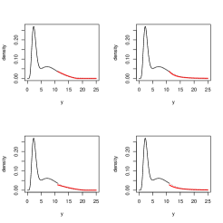
Figure 1: Probability density function of the model (3) for a number of parameters values: (a) $\xi=-0.4$ and $\sigma=3$, (b) $\xi=0.4$ and $\sigma=3$, (c) $\xi=-0.4$ and $\sigma=4$ and (d) $\xi=0.4$ and $\sigma=4$, threshold $u=11$ and the center of the densities is a mixture of two gamma densities the tails are modelling with GPD.

Figure 1. displays the density of the proposed model considering different values in the parameters. This model allows a discontinuity of the density at the threshold because constrains are basically solve defining the adequate models we consider in this paper for the posterior analysis in the tail (see gammerman).

3 Simulation study

In this section we evaluate the performance of the proposed model through a simulation study. The precision $\alpha$ of $g_{0}$ in the DP affects the expected number of components in the mixture. Hanson consider values of $\alpha$ fixed to 0.1 and 1 and also random values using different assignments of Gamma priors for $\alpha$ such as $\Gamma(2,2)$ and $\Gamma(2,0.5)$. Here we consider the precision for DP using $\alpha=0.1$. The hyperparameters of $g_{0}$ can be expressed in terms of the mean $\mu=\lambda/\gamma$ and variance $V=\lambda/\gamma^{2}$ of $h(x|\theta)$ (see Hanson) as two diffuse densities $f(\mu|a_{\lambda},a_{\gamma})=a_{\lambda}a_{\gamma}/(a_{\lambda}\mu+a_{\gamma})^{2}$ and $f(V^{-1}|a_{\lambda},a_{\gamma})=\Gamma(2,a_{\lambda}\mu^{2}+a_{\gamma}\mu)$ respectively. Suppose now that $a_{\lambda}=a_{\gamma}=1$, so $f(\mu|1,1)=1/(1+\mu)^{2}$ which is the Beta Prime distribution with hyperparamters of scale and shape equals to 1. The Beta prime distribution has been used as default density for modelling inference in Bayesian analysis. Therefore we can think that we are modelling the mean of the mixture of gammas densities in a non informative (but robust) manner. We consider a small sample size $n=200$. Hanson obtain an accurate smooth in an univariate density using DPMG with different specifications for $\alpha$ and large sample sizes 1000 and 10000. Here, we have that $\xi=0.4$, $\sigma=3$ and the threshold $u=11$ at the 90% quantile in the simulated data. The simulated mixture density for the central part is:

$$h(x)=0.5\Gamma(x|10,4)+0.5\Gamma(x|6,0.7).$$ (13)

Following Hanson the hyperparameters for $a_{\lambda}$ and $a_{\gamma}$ are $b_{\lambda}=b_{\gamma}=c_{\lambda}=c_{\gamma}=0.001$ in order to have a non informative $g_{0}$. The prior of the threshold $u$ has mean equal to 90% quantile in the simulated data and the variance $\sigma^{2}_{u}$ gives 99% of probability in the range between 50% and 99% of the simulated data. As usual in the Metropolis algorithm, we adjust the variance of the sampling proposal densities considering the hessian of the maximum likelihood estimates using some MCMC simulations. We obtained convergence of all parameters using 10000 iterations after a burn-in period of 5000 iterations. Figures 2 displays the quality of the approach even with a small sample size of $n=200$. The posterior density in the proposed model reproduces the underline density with precision according to the credible interval in the bulk part and posterior predictive mean in the tail. The density estimation in bulk part of the proposed model could be even better when large sample sizes are considered (see Hanson). Figure 3 displays the posterior densities of threshold $u$, scale $\sigma$, and shape $\xi$. We can see the posterior distribution represents nicely the true parameters. In particular the threshold is centered around the true value 11. Figures 4 shows as the posterior distributions of the predictive quantiles at 95% is accurately estimated.

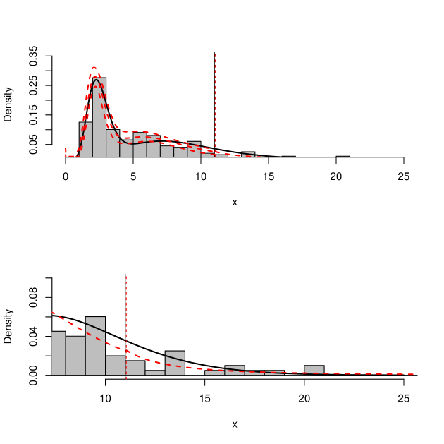
Figure 2: Dashed red line: Posterior predictive density using the Dirichlet process mixture of gamma densities in the bulk part and a GPD in the tail. Full black line is the true density and the dashed red line is the simulated density. The histogram displays the simulated data. The vertical full black line is the true threshold location and the vertical dashed red line is the posterior threshold location.

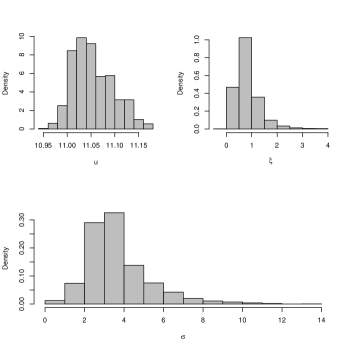
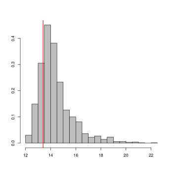
Figure 3: Posterior distribution of $u$, $\xi$ and $\sigma$.

Figure 4: Posterior histogram of the 95% quantile for the simulation. Red line the true quantile.

4 Application to the flow levels in the Gurabo river

River flow levels are important measures to prevent disasters in populations when flow rate exceeds the capacity of the river channel. We applied the proposed model in river flow levels measured at cubic feet per second ($ft^{3}/s$) in Gurabo river at Gurabo Puerto Rico. The data is available at waterdata.usgs.gov. The flows are monitoring between December 2 2012, 12:00 am to December 4 2012, 8:45 pm. The measures are made each 15 minutes for a total sample size of n=254. We obtained convergence of all parameters using 5000 iterations after a burn-in period of 2000 iterations.

Figure 5 displays the posterior distributions of the parameters in the tail of the proposed model. The threshold, scale and shape are around of 1430 (quantile at 96% according to the simulation), 300 and -0.25. Figure 6 shows the posterior distribution for the 99.9% high quantile, we can see the maximum value is less than the posterior mean for the quantile at 99.9% and the posterior distribution is asymmetric which is expected. Figure 7 displays the posterior density using DPMG in the bulk part and a GPD in the tail. We can see our proposed model reproduces the data in the bulk and tail parts. As a conclusion according to the posterior analysis (based on the last two days) with a probability of 0.1% we can see values bigger than approximately 1998 $ft^{3}/s$ in the Gurabo River.

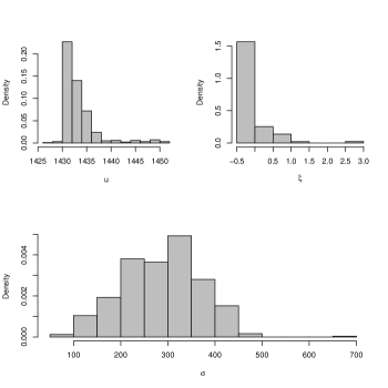
Figure 5: Posterior histogram of the GPD parameters in the tail of the proposed model for the application.

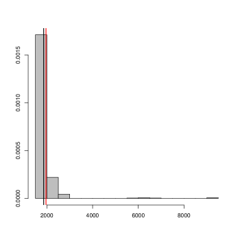
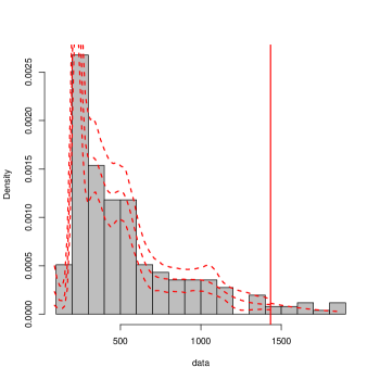
Figure 6: Posterior distribution of the 99.9% quantile for the application. Black line the maximum observed data and red line the posterior mean for the 99.9% simulated quantile.

Figure 7: Posterior density using the Dirichlet process mixture of gamma densities in the bulk part and posterior predictive distribution using a GPD in the tail. The vertical red line is the posterior threshold location.

5 Conclusion

We proposed a model with a Dirichlet process mixture of gamma densities in the bulk part of the distribution and a heavy tailed generalized Pareto distribution in the tail for extreme value estimation. The proposal is very flexible and simple for density estimation in the bulk part and posterior inference in the tail. According to the simulations and application to real data the model works well even for small sample sizes and in the absence of prior information. The Dirichlet Process mixture controls the expected number of components and so the extensive task for model comparison purposes using BIC and DIC criteria on a fixed number of gamma components in the bulk part is not necessary. The proposed model was applied to a real environmental data set but interesting applications can be found in different areas such as clinical trials or finance.

Appendix A MCMC algorithm

1. For the bulk part we need to compute $h(x|\theta)$ and also $H(u|\theta)$, we consider the pólya urn expression in the DPMG to compute posterior realizations for the density $h(x|\theta)$. Let $\{\theta_{1}^{*},...,\theta^{*}_{n^{*}}\}$ the unique values of $\theta_{i}$, $\omega_{i}=j$ if and only if $\theta_{i}=\theta_{j}^{*}$ $i=1,2,,...,n$ and $n_{j}=|\{i:\omega_{i}=j\}|$ and $j=1,2,...,n^{*}$ with $n^{*}$ number of distinct values. We use the following transition probabilities:

   1. Pólya urn: marginalized $G$ (using ^- to indicate summaries without $\omega_{i}$) and defining a specific configuration $\{\omega_{1},..,\omega_{n}\}$ with transition probabilities:

      $$p(\omega_{i}=\ell|\omega_{-i})\propto\begin{cases}n_{j}^{-}&j=1,...,n^{*-},\\ \alpha&j=n^{*-}+1\end{cases}$$ (14)

   2. Resampling cluster membership indicators $\omega_{i}$:

      $$\small p(\omega_{i}=j|,...,x_{i})\propto\begin{cases}n_{j}^{-}k(x_{i};\theta_{j}^{*})&j=1,...,n^{*-},\\ \alpha\int k(x_{i};\theta_{i})dG_{0}(\theta_{i}|\eta)&j=n^{*-}+1\end{cases}$$ (15)

      where we use the close results in Hanson:

      $$k(x_{i};\theta_{j}^{*}) =h(x_{i}|\theta_{j}^{*})$$ (16)

      $$\small\int k(x_{i};\theta_{i})dG_{0} (\theta_{i}|\mu,\tau^{2})=$$ (17)

      $$\frac{a_{\lambda}a_{\gamma}}{x_{i}(x_{i}+a_{\lambda})(a_{\lambda}-\log(x_{i}/(x_{i}+a_{\gamma})))^{2}}$$ (18)

      with probability proportional to $n_{j}^{-}k(x_{i};\theta_{j}^{*})$ we make $\theta_{i}=\theta_{j}^{*-}$. On the other hand with probability proportional to $\alpha\int k(y_{i};\theta_{i},\phi)dG_{0}(\theta_{i}|\eta)$ we open a new component and we sample $\theta_{i}=(\lambda_{i},\gamma_{i})$. First we sample $\lambda_{i}|\eta\sim\Gamma(2,a_{\lambda}-\log(x_{i}/(x_{i}+a_{\gamma}))^{2})$ then we sample $\gamma_{i}|\lambda_{i},\eta\sim\Gamma(\lambda_{i}+1,x_{i}+a_{\gamma})$.

2. Now we are interested in to show the sampling for the parameters in the GPD defined in the tails of (2). Following gammerman we compute the posterior distribution of $u$, $\xi$ and $\sigma$ using three steeps of the Metropolis Hasting algorithm. The algorithm is as follow:

   1. Sampling $\xi$: proposal transition kernel is given by a truncated normal

      $$\xi^{*}|\xi^{b}\sim N(\xi^{s},V_{\xi})I(-\sigma^{b}/(M-u^{b}),\infty)$$ (19)

      where $V_{\xi}$ is a variance in order to improve the mixing. $M$ is the maximum value in the sample the acceptance probability is

      $$\small\alpha_{\xi}=\min\left\{1,\dfrac{p(\theta^{*},\phi^{*}|x)\Phi((\xi^{b}+\sigma^{b}/(M-u^{b}))/\sqrt{V_{\xi}})}{p(\theta^{b},\phi^{b}|x)\Phi((\xi^{*}+\sigma^{*}/(M-u^{*}))/\sqrt{V_{\xi}})}\right\}$$

      where is the density function of the standard normal distribution.

   2. Sampling $\sigma$: If $\xi^{(b+1)}>0$ then $\sigma^{*}$ is sampled from the Gamma distribution $\Gamma(\sigma^{2(b)}/V_{\sigma},\sigma^{b}/V_{\sigma})$ where $V_{\sigma}$ is a variance in order to improve the mixing. On the other hand if $\xi^{(b+1)}<0$ then $\sigma^{*}$ is sampled from a truncated normal

      $$\sigma^{*}|\sigma^{b}\sim N(\sigma^{s},V_{\sigma})I(-\xi^{(b+1)}(M-u^{b}),\infty)$$ (20)

      the acceptance probabilities are respectively:

      $$\small\alpha_{\sigma}=\min\left\{1,\dfrac{p(\theta^{*},\phi^{*}|x)\Phi((\sigma^{b}+\xi^{(b+1)}(M-u^{b})/\sqrt{V_{\sigma}})}{p(\theta^{b},\phi^{b}|x)\Phi((\sigma^{*}+\xi^{(b+1)}(M-u^{b})/\sqrt{V_{\sigma}})}\right\}$$

      and

      $$\small\alpha_{\sigma}=\min\left\{1,\dfrac{p(\theta^{*},\phi^{*}|x)\Gamma(\sigma^{b}|\sigma^{2(*)}/V_{\sigma},\sigma^{*}/V_{\sigma})}{p(\theta^{b},\phi^{b}|x)\Gamma(\sigma^{*}|\sigma^{2(b)}/V_{\sigma},\sigma^{(b)}/V_{\sigma})}\right\}$$

   3. The threshold $u^{*}$ is sampled following the requirement of the lower truncation for the GPD. Therefore $u^{*}$ is sampled using a truncated normal density

      $$\sigma^{*}|\sigma^{b}\sim N(u^{s},V_{u})I(a^{(b+1)},\infty)$$ (21)

      If $\xi^{(b+1)}\geq 0$ then $a^{(b+1)}$ is the minimum value at the sample in the iteration $b+1$ otherwise if $\xi^{(b+1)}<0$ $a^{(b+1)}=M+\sigma^{(b+1)}/\xi^{(b+1)}$. The acceptance probability is then

      $$\small\alpha_{\xi}=\min\left\{1,\dfrac{p(\theta^{*},\phi^{*}|x)\Phi((u^{b}-a^{b+1})/\sqrt{V_{u}})}{p(\theta^{b},\phi^{b}|x)\Phi((u^{b}-a^{b+1})/\sqrt{V_{u}})}\right\}$$

References

- [1] \harvarditemAntoniak1974Antoniak Antoniak, C. E. \harvardyearleft1974\harvardyearright, ‘Mixture of Dirichlet process with applications to Bayesian nonparametric problems’, Annals of Statistics 2, 1152–1174.
- [2] \harvarditem[Behrens et al.]Behrens, Lopez \harvardand Gammerman2004Behrens Behrens, C. N., Lopez, H. F. \harvardand Gammerman, D. \harvardyearleft2004\harvardyearright, ‘Bayesian analysis of extreme events with threshold estimation’, Statistical Modelling 4, 227–244.
- [3] \harvarditemCarreu \harvardand Bengio2009carreu Carreu, J. \harvardand Bengio, Y. \harvardyearleft2009\harvardyearright, ‘A hibrid Pareto mixture for conditional asymmetric fat-tailed data’, Extremes 12, 53–76.
- [4] \harvarditemCastellanos \harvardand Cabras1996coles Castellanos, E. \harvardand Cabras, S. \harvardyearleft1996\harvardyearright, ‘A Bayesian analysis of extreme rainfall data’, Applied Statistics 45, 463–478.
- [5] \harvarditemCastellanos \harvardand Cabras2007catellanos Castellanos, E. \harvardand Cabras, S. \harvardyearleft2007\harvardyearright, ‘A default Bayesian procedure for the generalized Pareto distribution’, Journal of Statistical Planing and Inference 137, 473–483.
- [6] \harvarditem[do Nacimiento et al.]do Nacimiento, Gammerman \harvardand Freitas2011gammerman do Nacimiento, F., Gammerman, D. \harvardand Freitas, H. \harvardyearleft2011\harvardyearright, ‘A semiparametric Bayesian approach to extreme value estimation’, Statist. Comput. .
- [7] \harvarditemEscobar \harvardand West1995escobar Escobar, M. \harvardand West, M. \harvardyearleft1995\harvardyearright, ‘Bayesian density estimation and inference using mixtures’, Journal of the American Statistical Association 90, 577–588.
- [8] \harvarditemFerguson1973Ferguson Ferguson, T. \harvardyearleft1973\harvardyearright, ‘A Bayesian analysis of some nonparametric problems’, Annals of Statistics 1, 209–230.
- [9] \harvarditem[Frigessi et al.]Frigessi, Haug \harvardand Harvard2003friguessi Frigessi, A., Haug, O. \harvardand Harvard, R. \harvardyearleft2003\harvardyearright, ‘A dynamic mixture model for unsupervised tail estimation without threshold estimation’, Extremes 5, 219–235.
- [10] \harvarditemHanson2006Hanson Hanson, T. E. \harvardyearleft2006\harvardyearright, ‘Modelling censoring lifetime data using a mixture of Gamma baselines’, Bayesian Analysis 3, 576–592.
- [11] \harvarditem[MacDonald et al.]MacDonald, Scarrot, Lee, B., Reale \harvardand Rusell2011Macdonald MacDonald, A., Scarrot, C. J., Lee, D., B., D., Reale, M. \harvardand Rusell, G. \harvardyearleft2011\harvardyearright, ‘A flexible extreme value mixture model’, Computational statistics and data analysis 55, 2137–2157.
- [12] \harvarditemMacEachern1994miki MacEachern, S. \harvardyearleft1994\harvardyearright, ‘Estimating normal means with a conjugate style Dirichlet process prior’, Communications in statistics 23(460), 727–741.
- [13] \harvarditemScarrot \harvardand MacDonnald2012mamamia Scarrot, C. \harvardand MacDonnald, A. \harvardyearleft2012\harvardyearright, ‘A review of extreme value threshold estimation and uncertainty quantification’, Statistical Journal 10, 33–60.
- [14] \harvarditem[Wiper et al.]Wiper, Insua \harvardand Ruggeri2001wiper Wiper, M., Insua, D. R. \harvardand Ruggeri, F. \harvardyearleft2001\harvardyearright, ‘Mixture of Gamma distributions with applications’, Journal of the American statistical association 10, 440–454.
- [15]