Efficient estimation in sufficient dimension reduction

Abstract

We develop an efficient estimation procedure for identifying and estimating the central subspace. Using a new way of parameterization, we convert the problem of identifying the central subspace to the problem of estimating a finite dimensional parameter in a semiparametric model. This conversion allows us to derive an efficient estimator which reaches the optimal semiparametric efficiency bound. The resulting efficient estimator can exhaustively estimate the central subspace without imposing any distributional assumptions. Our proposed efficient estimation also provides a possibility for making inference of parameters that uniquely identify the central subspace. We conduct simulation studies and a real data analysis to demonstrate the finite sample performance in comparison with several existing methods.

and t1Supported by NSF Grants DMS-12-06693 and DMS-10-00354 and the National Institute of Neurological Disorders and Stroke Grant R01-NS073671. t2Supported by Natural Science Foundation of China (11071077), Innovation Program of Shanghai Municipal Education Commission (13ZZ055), Pujiang Project of Science and Technology Commission of Shanghai Municipality (12PJ1403200) and Grants for New Century Excellent Talents in University, Ministry of Education (NCET-12-0901). All the correspondence should be directed to Liping Zhu at e2.

1 Introduction

Consider a general model in which the univariate response variable $Y$ is assumed to depend on the $p$-dimensional covariate vector $\mathbf{x}$ only through a small number of linear combinations $\bolds{\beta}^{\mathrm{T}}\mathbf{x}$, where $\bolds{\beta}$ is a $p\times d$ matrix with $d<p$. In this model, how $Y$ depends on $\bolds{\beta}^{\mathrm{T}}\mathbf{x}$ is left unspecified. It is not difficult to see that $\bolds{\beta}$ is not identifiable. The quantity of general interest is usually the column space of $\bolds{\beta}$, which is termed the central subspace if $d$ is the smallest possible value to satisfy the model assumption Cook1998 .

This general model was proposed by Li Li1991 and has attracted much attention in the last two decades. It generated the field of sufficient dimension reduction Cook1998 , in which the main interest is to estimate the central subspace consistently. Influential works in this area include, but are not limited to, sliced inverse regression Li1991 , sliced average variance estimation CookWeisberg1991 , directional regression LiWang2007 , the generalization of the aforementioned methods to nonelliptically distributed predictors LiDong2009 , DongLi2010 , Fourier transformation ZhuZeng2006 , cumulative slicing estimators ZhuZhuFeng2010 and conditional density based minimum average variance estimation Xia2007 , etc.

Despite the various estimation methods, it is unclear if any of these estimators are optimal in the sense that they can exhaustively estimate the entire central subspace and have the minimum possible asymptotic estimation variance. To the best of our knowledge, the efficiency issue has never been discussed in the context of sufficient dimension reduction.

In this paper we study the estimation and inference in sufficient dimension reduction. We propose a simple parameterization so that the central subspace is uniquely identified by a $(p-d)d$-dimensional parameter that is not subject to any constraints. Thus we convert the problem of identifying the central subspace into a problem of estimating a finite dimensional parameter in a semiparametric model. This allows us to derive the estimation procedures and perform inference using semiparametric tools. How to make inference about the central subspace is a challenging issue. This is partially caused by the complexity of estimating a space rather than a parameter. Our new parameterization overcomes this complexity and permits a relatively straightforward calculation of the estimation variability.

We further construct an efficient estimator, which reaches the minimum asymptotic estimation variance bound among all possible consistent estimators. Efficiency bounds are of fundamental importance to the theoretical consideration. Such bounds quantify the minimum efficiency loss that results from generalizing one restrictive model to a more flexible one, and hence they can be important in making the decision of which model to use. The efficiency bounds also provide a gold standard by which the asymptotic efficiency of any particular semiparametric estimator can be measured Newey1990 . Generally speaking, a semiparametric efficient estimator is usually the ultimate destination when searching for consistent estimators or trying to improve existing procedures. When an efficient estimator is obtained, the procedure of estimation can be considered to have reached certain optimality.

In the literature, vast and significant effort has been devoted to studying the semiparametric efficiency bounds for consistent estimators in semiparametric models. The simplest and most familiar examples are the ordinary and weighted least square estimators in the linear regression setting. Efficiency issues are also considered in more complex semiparametric problems such as regressions with missing covariates RobinsRotnitzkyZhao1994 , skewed distribution families MaGentonTsiatis2005 , MaHart2007 , measurement error models TsiatisMa2004 , MaCarroll2006 , partially linear models MaChiouWang2006 , the Cox model Tsiatis2006 , page 113, accelerated failure model ZengLin2007a or other general survival models ZengLin2007b and latent variable models MaGenton2010 .

One typical semiparametric tool is to obtain estimators through obtaining the corresponding influence functions. In deriving the influence function family and its efficient member, we use the geometric technique illustrated in BickelKlaassenRitovWellner1993 and Tsiatis2006 . All our derivations are performed without using the linearity or constant variance condition that is often assumed in the dimension reduction literature. Our analysis is thus readily applicable when some covariates are discrete or categorical. In summary, we provide an efficient estimator which can exhaustively estimate the central subspace without imposing any distributional assumptions on the covariate $\mathbf{x}$.

The rest of this paper is organized as follows. In Section 2, we propose a simple parameterization of the central subspace and highlight the semiparametric approach to estimating the central subspace. We also derive the efficient score function. In Section 3, we present a class of locally efficient estimators and identify the efficient member. We illustrate how to implement the efficient estimator to reach the optimal efficiency bound. Simulation studies are conducted in Section 4 to demonstrate the finite sample performance and the method is implemented in a real data example in Section 5. We finish the paper with a brief discussion in Section 6. All the technical derivations are given in a supplementary material supp .

2 The semiparametric formulation

2.1 Parameterization of central subspace

In the context of sufficient dimension reduction Li1991 , Cook1998 , one often assumes

$$F(y|\mathbf{x})=F\bigl{(}y|\bolds{\beta}^{\mathrm{T}}\mathbf{x}\bigr{)}\qquad\mbox{for }y\in\mathrm{R},$$ (1)

where $F(y|\mathbf{x})\stackrel{{\scriptstyle\mathrm{def}}}{{=}}\operatorname{Pr}(Y\leq y|\mathbf{x})$ is the conditional distribution function of the response $Y$ given the covariates $\mathbf{x}$, and $\bolds{\beta}$ is a $p\times d$ matrix as defined previously. The goal of sufficient dimension reduction is to estimate the column space of $\bolds{\beta}$, which is termed the dimension reduction subspace. Because a dimension reduction subspace is not necessarily unique, the primary interest is usually the central subspace $\mathcal{S}_{Y|\mathbf{x}}$, which is defined as the minimum dimension reduction subspace if it exists and is unique Cook1998 . The dimension of $\mathcal{S}_{Y|\mathbf{x}}$, denoted with $d$, is commonly referred to as the structural dimension. Similarly to Cook1994 , we exclude a pathological case where there exists a vector $\bolds{\alpha}$ such that $\bolds{\alpha}^{\mathrm{T}}\mathbf{x}$ is a deterministic function of $\bolds{\beta}^{\mathrm{T}}\mathbf{x}$ while $\bolds{\alpha}$ does not belong to the column space of $\bolds{\beta}$.

The central subspace $\mathcal{S}_{Y|\mathbf{x}}$ has a well-known invariance property Cook1998 ,page 106, that is, $\mathcal{S}_{Y|\mathbf{x}}=\mathbf{D}\mathcal{S}_{Y|{\mathbf{z}}}$, where $\mathbf{z}=\mathbf{D}^{\mathrm{T}}\mathbf{x}+\mathbf{b}$ for any $p\times p$ nonsingular matrix $\mathbf{D}$ and any length $p$ vector $\mathbf{b}$. This allows us to assume throughout that the covariate vector $\mathbf{x}$ satisfies $E(\mathbf{x})=\mathbf{0}$ and $\operatorname{cov}(\mathbf{x})=\mathbf{I}_{p}$. Identifying $\mathcal{S}_{Y|\mathbf{x}}$ is the essential interest of sufficient dimension reduction for model (1). Typically, $\mathcal{S}_{Y|\mathbf{x}}$ is identified through estimating a basis matrix $\bolds{\beta}\in\mathrm{R}^{p\times d}$ of minimal dimension that satisfies (1). Although $\mathcal{S}_{Y|\mathbf{x}}$ is unique, the basis matrix $\bolds{\beta}$ is clearly not. In fact, for any $d\times d$ full rank matrix $\mathbf{A}$, $\bolds{\beta}\mathbf{A}$ generates the same column space as $\bolds{\beta}$. Thus, to uniquely map one central subspace $\mathcal{S}_{Y|\mathbf{x}}$ to one basis matrix, we need to focus on one representative member of all the $\bolds{\beta}\mathbf{A}$ matrices generated by different $\mathbf{A}$’s. We write $\bolds{\beta}=(\bolds{\beta}_{u}^{\mathrm{T}},\bolds{\beta}_{l}^{\mathrm{T}})^{\mathrm{T}}$, where the upper submatrix $\bolds{\beta}_{u}$ has size $d\times d$ and the lower submatrix $\bolds{\beta}_{l}$ has size $(p-d)\times d$. Because $\bolds{\beta}$ has rank $d$, we can assume without loss of generality that $\bolds{\beta}_{u}$ is invertible. The advantage of using $\bolds{\beta}\bolds{\beta}_{u}^{-1}$ is that its upper $d\times d$ submatrix is the identity matrix, while the lower $(p-d)\times d$ matrix can be any matrix. In addition, two matrices $\bolds{\beta}_{1}\bolds{\beta}_{1u}^{-1}$ and $\bolds{\beta}_{2}\bolds{\beta}_{2u}^{-1}$ are different if and only if the column spaces of $\bolds{\beta}_{1}$ and $\bolds{\beta}_{2}$ are different. Therefore, if we consider the set of all the $p\times d$ matrices $\bolds{\beta}$ where the upper $d\times d$ submatrix is the identity matrix $\mathbf{I}_{d}$, it has a one-to-one mapping with the set of all the different central subspaces. Thus, as long as we restrict our attention to the set of all such matrices, the problem of identifying $\mathcal{S}_{Y|\mathbf{x}}$ is converted to the problem of estimating $\bolds{\beta}_{l}$, which contains $p_{t}=(p-d)d$ free parameters. Note that $p_{t}$ is the dimension of the Grassmann manifold formed by the column spaces of all different $\bolds{\beta}$ matrices. Thus, we can view $\bolds{\beta}_{l}$ as a unique parameterization of the manifold. Here the subscript “_t” stands for total. For notational convenience in the remainder of the text, for an arbitrary $p\times d$ matrix $\bolds{\beta}=(\bolds{\beta}_{u}^{\mathrm{T}},\bolds{\beta}_{l}^{\mathrm{T}})^{\mathrm{T}}$, we define the concatenation of the columns contained in the lower $p-d$ rows of $\bolds{\beta}$ as $\operatorname{vecl}(\bolds{\beta})=\operatorname{vec}(\bolds{\beta}_{l})=(\beta_{d+1,1},\ldots,\beta_{p,1},\ldots,\beta_{d+1,d},\ldots,\beta_{p,d})^{\mathrm{T}}$, where in the notation $\operatorname{vecl}$, “vec” stands for vectorization, and “l” stands for the lower part of the original matrix. We then can write the concatenation of the parameters in $\bolds{\beta}$ as $\operatorname{vecl}(\bolds{\beta})$. Thus, from now on, we only consider basis matrix of $\mathcal{S}_{Y|\mathbf{x}}$ that has the form $\bolds{\beta}=(\mathbf{I}_{d},\bolds{\beta}_{l}^{\mathrm{T}})^{\mathrm{T}}$, where $\bolds{\beta}_{l}$ is a $(p-d)\times d$ matrix. Estimating the parameters in $\bolds{\beta}$ is a typical semiparametric estimation problem, in which the parameter of interest is $\operatorname{vecl}(\bolds{\beta})$. Therefore we have converted the problem of estimating the central space $\mathcal{S}_{Y|\mathbf{x}}$ into a problem of semiparametric estimation.

Remark 1.

The above parameterization of $\mathcal{S}_{Y|\mathbf{x}}$ excludes the pathological case where one or more of the first $d$ covariates do not contribute to the model or contribute to the model through a fixed linear combination. When this happens, $\bolds{\beta}_{u}$ will be singular. However, because $\bolds{\beta}$ has rank $d$, hence if this happens, one can always rotate the order of the covariates (hence rotate the rows of $\bolds{\beta}$) to ensure that after rotation, the resulting $\bolds{\beta}_{u}$ has full rank.

2.2 Efficient score

In this section we derive the efficient score for estimating $\bolds{\beta}$ under the above parameterization. That is, we now consider model (1), where $\bolds{\beta}=(\mathbf{I}_{d},\bolds{\beta}_{l}^{\mathrm{T}})^{\mathrm{T}}$ and $\mathbf{x}$ satisfies $E(\mathbf{x})=\mathbf{0}$ and $\operatorname{var}(\mathbf{x})=\mathbf{I}_{p}$. The general semiparametric technique we use is originated from BickelKlaassenRitovWellner1993 and is wonderfully presented in Tsiatis2006 . Using this approach, we obtain the main result of this section, that we can use (2) to obtain an efficient estimation of $\bolds{\beta}$.

The likelihood of one random observation $(\mathbf{x},Y)$ in (1) is $\eta_{1}(\mathbf{x})\eta_{2}(Y,\bolds{\beta}^{\mathrm{T}}\mathbf{x})$, where $\eta_{1}$ is a probability mass function (p.m.f.) or a probability density function (p.d.f.) of $\mathbf{x}$, or a mixture, depending on whether $\mathbf{x}$ contains discrete variables, and $\eta_{2}$ is the conditional p.m.f./p.d.f. of $Y$ on $\mathbf{x}$. We view $\eta_{1},\eta_{2}$ as infinite dimensional nuisance parameters and $\operatorname{vecl}(\bolds{\beta})$ as the $p_{t}$-dimensional parameter of interest. Following the semiparametric analysis procedure, we first derive the nuisance tangent space $\Lambda=\Lambda_{1}\oplus\Lambda_{2}$, where

$$\Lambda_{1} = \bigl{\{}\mathbf{f}(\mathbf{x})\dvtx\forall\mathbf{f}\mbox{ such that }E(\mathbf{f})=\mathbf{0}\bigr{\}},$$

$$\Lambda_{2} = \bigl{\{}\mathbf{f}\bigl{(}Y,\bolds{\beta}^{\mathrm{T}}\mathbf{x}\bigr{)}\dvtx\forall\mathbf{f}\mbox{ such that }E(\mathbf{f}|\mathbf{x})=E\bigl{(}\mathbf{f}|\bolds{\beta}^{\mathrm{T}}\mathbf{x}\bigr{)}=\mathbf{0}\bigr{\}}.$$

Here, the notation $\oplus$ means the usual addition of the two spaces $\Lambda_{1}$, $\Lambda_{2}$, while $\Lambda_{1}$ and $\Lambda_{2}$ have the extra property that they are orthogonal to each other. This means the inner product of two arbitrary functions from $\Lambda_{1}$ and $\Lambda_{2}$, respectively, calculated as the covariance between them, is zero. We then obtain its orthogonal complement

$$\Lambda^{\perp}=\bigl{\{}\mathbf{f}(Y,\mathbf{x})-E\bigl{(}\mathbf{f}|\bolds{\beta}^{\mathrm{T}}\mathbf{x},Y\bigr{)}\dvtx E(\mathbf{f}|\mathbf{x})=E\bigl{(}\mathbf{f}|\bolds{\beta}^{\mathrm{T}}\mathbf{x}\bigr{)},\forall\mathbf{f}\bigr{\}}.$$

The detailed derivation of $\Lambda$ and $\Lambda^{\perp}$ is given in Appendix A.2 of MaZhu2012 . The form of $\Lambda^{\perp}$ permits many possibilities for constructing estimating equations. For example, for arbitrary functions $\mathbf{g}_{i}$ and $\bolds{\alpha}_{i}$, the linear combination

$$\sum_{i=1}^{k}\bigl{\{}\mathbf{g}_{i}\bigl{(}Y,\bolds{\beta}^{\mathrm{T}}\mathbf{x}\bigr{)}-E\bigl{(}\mathbf{g}_{i}|\bolds{\beta}^{\mathrm{T}}\mathbf{x}\bigr{)}\bigr{\}}\bigl{\{}\bolds{\alpha}_{i}(\mathbf{x})-E\bigl{(}\bolds{\alpha}_{i}|\bolds{\beta}^{\mathrm{T}}\mathbf{x}\bigr{)}\bigr{\}}$$

will provide a consistent semiparametric estimator since it is a valid element in $\Lambda^{\perp}$. This form is exploited extensively in MaZhu2012 to establish links between the semiparametric approach and various inverse regression methods. Among all elements in $\Lambda^{\perp}$, the most interesting one is the efficient score, defined as the orthogonal projection of the score vector $\mathbf{S}_{\beta}$ onto $\Lambda^{\perp}$. We write the efficient score as $\mathbf{S}_{\mathrm{eff}}=\Pi(\mathbf{S}_{\beta}|\Lambda^{\perp})$. Because the efficient score can be normalized to the efficient influence function, it enables us to construct an efficient estimator of $\operatorname{vecl}(\bolds{\beta})$ which reaches the optimal semiparametric efficiency bound in the sense of BickelKlaassenRitovWellner1993 . In the supplementary document supp , we derive the efficient score function to be

$$\qquad\mathbf{S}_{\mathrm{eff}}\bigl{(}Y,\mathbf{x},\bolds{\beta}^{\mathrm{T}}\mathbf{x},\eta_{2}\bigr{)}=\operatorname{vecl}\biggl{[}\bigl{\{}\mathbf{x}-E\bigl{(}\mathbf{x}|\bolds{\beta}^{\mathrm{T}}\mathbf{x}\bigr{)}\bigr{\}}\frac{\partial\log\{\eta_{2}(Y,\bolds{\beta}^{\mathrm{T}}\mathbf{x})\}}{\partial(\mathbf{x}^{\mathrm{T}}\bolds{\beta})}\biggr{]}.$$ (2)

Hypothetically, the efficient estimator can be obtained through implementing

$$\sum_{i=1}^{n}\mathbf{S}_{\mathrm{eff}}\bigl{(}Y_{i},\mathbf{x}_{i},\bolds{\beta}^{\mathrm{T}}\mathbf{x}_{i},\eta_{2}\bigr{)}=\mathbf{0}.$$

However, $\mathbf{S}_{\mathrm{eff}}$ is not readily implementable because it contains the unknown quantities $E(\mathbf{x}|\mathbf{x}^{\mathrm{T}}\bolds{\beta})$ and $\partial\log\eta_{2}(Y,\bolds{\beta}^{\mathrm{T}}\mathbf{x})/\partial(\mathbf{x}^{\mathrm{T}}\bolds{\beta})$. For this reason, we first discuss a simpler alternative in the following section.

3 Locally efficient and efficient estimators

3.1 Locally efficient estimators

We now discuss how to construct a locally efficient estimator. This is an estimator that contains some subjectively chosen components. If the components are “well” chosen, the resulting estimator is efficient. Otherwise, it is not efficient, but still consistent. The efficient estimator defined in (2) requires one to estimate $\eta_{2}$, the conditional p.d.f. of $Y$ on $\bolds{\beta}^{\mathrm{T}}\mathbf{x}$, and its first derivative with respect to $\bolds{\beta}^{\mathrm{T}}\mathbf{x}$. Although this is feasible, as we will describe in detail in Section 3.2, it certainly is not a trivial task as it involves several nonparametric estimations. Because of this, a compromise is to consider an estimator that depends on a posited model of $\eta_{2}$. Specifically, we would choose some favorite form for $\eta_{2}$, denoted $\eta_{2}^{*}(Y,\bolds{\beta}^{\mathrm{T}}\mathbf{x})$, and utilize it in place of $\eta_{2}$ to construct an estimating equation. If the posited model is correct (i.e., $\eta_{2}^{*}=\eta_{2}$), then we would have the optimal efficiency using the corresponding $\mathbf{S}_{\mathrm{eff}}^{*}$. However, even if the posited model is incorrect (i.e., $\eta_{2}^{*}\neq\eta_{2}$), we would still have consistency using the corresponding $\mathbf{S}_{\mathrm{eff}}^{*}$. A valid choice of $\mathbf{S}_{\mathrm{eff}}^{*}$ that indeed guarantees such property is

$$\mathbf{S}_{\mathrm{eff}}^{*}\bigl{(}Y_{i},\mathbf{x}_{i},\bolds{\beta}^{\mathrm{T}}\mathbf{x}_{i},\eta_{2}^{*}\bigr{)}$$

$$\qquad=\operatorname{vecl}\biggl{(}\bigl{\{}\mathbf{x}_{i}-E\bigl{(}\mathbf{x}_{i}|\bolds{\beta}^{\mathrm{T}}\mathbf{x}_{i}\bigr{)}\bigr{\}}$$

$$\hskip 56.0pt{}\times\biggl{[}\frac{\partial\log\{\eta_{2}^{*}(Y_{i},\bolds{\beta}^{\mathrm{T}}\mathbf{x}_{i})\}}{\partial(\mathbf{x}_{i}^{\mathrm{T}}\bolds{\beta})}-E\biggl{\{}\frac{\partial\log\eta_{2}^{*}(Y_{i},\bolds{\beta}^{\mathrm{T}}\mathbf{x}_{i})}{\partial(\mathbf{x}_{i}^{\mathrm{T}}\bolds{\beta})}\Big{|}\bolds{\beta}^{\mathrm{T}}\mathbf{x}_{i}\biggr{\}}\biggr{]}\biggr{)}.$$

When $\eta_{2}^{*}=\eta_{2}$, $E\{\partial\log\eta_{2}^{*}(Y_{i},\bolds{\beta}^{\mathrm{T}}\mathbf{x}_{i})/\partial(\mathbf{x}_{i}^{\mathrm{T}}\bolds{\beta})|\bolds{\beta}^{\mathrm{T}}\mathbf{x}_{i}\}=\mathbf{0}$, hence $\mathbf{S}_{\mathrm{eff}}^{*}=\mathbf{S}_{\mathrm{eff}}$. The construction of a locally efficient estimator is often useful in practice due to its relative simplicity. $\mathbf{S}_{\mathrm{eff}}^{*}$ is almost readily applicable except that the two expectations $E(\mathbf{x}_{i}|\bolds{\beta}^{\mathrm{T}}\mathbf{x}_{i})$ and $E\{\partial\log\eta_{2}^{*}(Y_{i},\bolds{\beta}^{\mathrm{T}}\mathbf{x}_{i})/\partial(\mathbf{x}_{i}^{\mathrm{T}}\bolds{\beta})|\bolds{\beta}^{\mathrm{T}}\mathbf{x}_{i}\}$ need to be estimated nonparametrically. One can use the familiar kernel or local polynomial estimators. In Theorem 1, we show that under mild conditions, with the two expectations estimated via the Nadaraya–Watson kernel estimators, the local efficiency property indeed holds and estimating the two expectations does not cause any difference from knowing them in terms of its first order asymptotic property.

We first present the regularity conditions needed for the theoretical development.

(The posited conditional density $\eta_{2}^{*}$). Denote $\mathbf{u}=\bolds{\beta}^{\mathrm{T}}\mathbf{x}$. The posited conditional density $\eta_{2}^{\ast}(Y,\mathbf{u})$ of $Y$ given $\mathbf{u}$ is bounded away from $0$ and infinity on its support $\mathcal{Y}$. The second derivative of $\log\eta_{2}^{\ast}(Y,\mathbf{u})$ with respect to $\mathbf{u}$ is continuous, positive definite and bounded. In addition, there is an open set $\bolds{\Omega}\in\mathrm{R}^{p_{t}}$ which contains the true parameter $\operatorname{vecl}(\bolds{\beta})$, such that the third derivative of $\eta_{2}(Y,\bolds{\beta}^{\mathrm{T}}\mathbf{x})$ satisfies

$$\bigl{|}\partial^{3}\bigl{\{}\eta_{2}^{\ast}\bigl{(}Y,\bolds{\beta}^{\mathrm{T}}\mathbf{x}\bigr{)}\bigr{\}}/\bigl{(}\partial\operatorname{vecl}(\bolds{\beta})_{j}\,\partial\operatorname{vecl}(\bolds{\beta})_{k}\,\partial\operatorname{vecl}(\bolds{\beta})_{l}\bigr{)}\bigr{|}\leq M_{jkl}^{\ast}(Y,\mathbf{x})$$

for all $\operatorname{vecl}(\bolds{\beta})\in\bolds{\Omega}$ and $1\leq j,k,l\leq p_{t}$, where $M_{jkl}^{\ast}(Y,\mathbf{x})$ satisfies $E\{{M_{jkl}^{\ast}}^{2}(Y,\break\mathbf{x})\}<\infty$, and $\beta_{j}$ is the $j$th component of $\operatorname{vecl}(\bolds{\beta})$.

(The nonparametric estimation). $E\{\partial\log\eta_{2}^{*}(Y,\bolds{\beta}^{\mathrm{T}}\mathbf{x})/\partial(\mathbf{x}^{\mathrm{T}}\bolds{\beta})|\bolds{\beta}^{\mathrm{T}}\mathbf{x}\}$ and $E(\mathbf{x}|\bolds{\beta}^{\mathrm{T}}\mathbf{x})$ are estimated via the Nadaraya–Watson kernel estimator. For simplicity, a common bandwidth $h$ is used which satisfies $nh^{8}\to 0$ and $nh^{2d}\to\infty$ as $n\to\infty$.

(The true conditional density $\eta_{2}$). The true conditional density$\eta_{2}(Y,\mathbf{u})$ of $Y$ given $\mathbf{u}$ is bounded away from $0$ and infinity on its support $\mathcal{Y}$. The first and second derivatives of $\log\eta_{2}$ satisfy

$$E\biggl{[}\frac{\partial\{\log\eta_{2}(Y,\bolds{\beta}^{\mathrm{T}}\mathbf{x})\}}{\partial\operatorname{vecl}(\bolds{\beta})}\biggr{]}=\mathbf{0}$$

and

$$E\biggl{[}\frac{\partial\{\log\eta_{2}(Y,\bolds{\beta}^{\mathrm{T}}\mathbf{x})\}}{\partial\operatorname{vecl}(\bolds{\beta})}\frac{\partial\{\log\eta_{2}(Y,\bolds{\beta}^{\mathrm{T}}\mathbf{x})\}}{\partial\operatorname{vecl}(\bolds{\beta})^{\mathrm{T}}}\biggr{]}=-E\biggl{[}\frac{\partial^{2}\{\log\eta_{2}(Y,\bolds{\beta}^{\mathrm{T}}\mathbf{x})\}}{\partial\operatorname{vecl}(\bolds{\beta})\,\partial\operatorname{vecl}(\bolds{\beta})^{\mathrm{T}}}\biggr{]}$$

is positive definite and bounded. In addition, there is an open set $\bolds{\Omega}\in\mathrm{R}^{p_{t}}$ which contains the true parameter $\operatorname{vecl}(\bolds{\beta})$, such that the third derivative of $\eta_{2}(Y,\bolds{\beta}^{\mathrm{T}}\mathbf{x})$ satisfies

$$\bigl{|}\partial^{3}\bigl{\{}\eta_{2}\bigl{(}Y,\bolds{\beta}^{\mathrm{T}}\mathbf{x}\bigr{)}\bigr{\}}/\bigl{(}\partial\operatorname{vecl}(\bolds{\beta})_{j}\,\partial\operatorname{vecl}(\bolds{\beta})_{k}\,\partial\operatorname{vecl}(\bolds{\beta})_{l}\bigr{)}\bigr{|}\leq M_{jkl}(Y,\mathbf{x})$$

for all $\operatorname{vecl}(\bolds{\beta})\in\bolds{\Omega}$ and $1\leq j,k,l\leq p_{t}$, where $M_{jkl}(Y,\mathbf{x})$ satisfies $E\{M_{jkl}^{2}(Y,\break\mathbf{x})\}<\infty$, and $\beta_{j}$ is the $j$th component of $\operatorname{vecl}(\bolds{\beta})$.

(The bandwidths). The bandwidths satisfy $h_{y}\to 0$, $b\to 0$ and $h_{x}\to 0$, and $nh_{y}^{d+2}b\to\infty$, $n^{1/2}\{h_{x}^{2}+(nh_{x}^{d})^{-1/2}\}\{h_{y}^{2}+b^{2}+(nh_{y}^{d+2}b)^{-1/2}\}\to 0$.

(The density functions of covariates). Let $\mathbf{u}=\bolds{\beta}^{\mathrm{T}}\mathbf{x}$. The density functions of $\mathbf{u}$ and $\mathbf{x}$ are bounded away from $0$ and infinity on their support $\mathcal{U}$ and $\mathcal{X}$ where ${\mathcal{U}}=\{\mathbf{u}=\bolds{\beta}^{\mathrm{T}}\mathbf{x}\dvtx\mathbf{x}\in{\mathcal{X}}\}$ and ${\mathcal{X}}$ is a compact support set of $\mathbf{x}$. Their second derivatives are finite on their supports.

(The smoothness). The regression functions $E(\mathbf{x}|\mathbf{u})$ has a bounded and continuous derivative on $\mathcal{U}$.

(The kernel function). The univariate kernel function $K(\cdot)$ is a bounded symmetric probability density function, has a bounded derivative and compact support $[-1,1]$, and satisfies $\mu_{2}=\int u^{2}K(u)\,du\neq 0$. The $d$-dimensional kernel function is a product of $d$ univariate kernel functions, that is, $K(\mathbf{u})=\prod_{j=1}^{d}K(u_{j})$, and $K_{h}(\mathbf{u})=\prod_{j=1}^{d}K_{h}(u_{j})=h^{-d}\prod_{j=1}^{d}K(u_{j}/h)$ for $\mathbf{u}=(u_{1},\ldots,u_{d})^{\mathrm{T}}$ and any bandwidth $h$.

Theorem 1.

Under conditions (A1)–(A2) and (C1)–(C3), the estimator obtained from the estimating equation

$$\sum_{i=1}^{n}\mathbf{S}_{\mathrm{eff}}^{*}\bigl{(}Y_{i},\mathbf{x}_{i},\bolds{\beta}^{\mathrm{T}}\mathbf{x}_{i},\eta_{2}^{*},\widehat{E}\bigr{)}=\mathbf{0}$$

is locally efficient. Specifically, the estimator is consistent if $\eta_{2}^{*}\neq\eta_{2}$, and is efficient if $\eta_{2}^{*}=\eta_{2}$. In addition, using the estimated $\widehat{E}(\cdot|\bolds{\beta}^{\mathrm{T}}\mathbf{x})$ results in the same estimation variance for $\operatorname{vecl}(\bolds{\beta})$ as using the true $E(\cdot|\bolds{\beta}^{\mathrm{T}}\mathbf{x})$. Specifically, the estimate $\widehat{\bolds}{\beta}$ satisfies

$$\sqrt{n}\bigl{\{}\operatorname{vecl}(\widehat{\bolds{\beta}})-\operatorname{vecl}(\bolds{\beta})\bigr{\}}\to N\bigl{\{}\mathbf{0},\mathbf{A}^{-1}\mathbf{B}\bigl{(}\mathbf{A}^{-1}\bigr{)}^{\mathrm{T}}\bigr{\}}$$

when $n\to\infty$, where

$$\mathbf{A}=E\biggl{\{}\frac{\partial\mathbf{S}_{\mathrm{eff}}^{*}(Y_{i},\mathbf{x}_{i},\bolds{\beta}^{\mathrm{T}}\mathbf{x}_{i},\eta_{2}^{*})}{\partial\operatorname{vecl}(\bolds{\beta})^{\mathrm{T}}}\biggr{\}},\qquad\mathbf{B}=E\bigl{\{}\mathbf{S}_{\mathrm{eff}}^{*}\bigl{(}Y_{i},\mathbf{x}_{i},\bolds{\beta}^{\mathrm{T}}\mathbf{x}_{i},\eta_{2}^{*}\bigr{)}^{\otimes 2}\bigr{\}}.$$

In Theorem 1 and thereafter, we use $\mathbf{v}^{\otimes 2}$ to denote $\mathbf{v}\mathbf{v}^{\mathrm{T}}$ for any matrix or vector $\mathbf{v}$, and use $\widehat{E}$ to denote the nonparametrically estimated expectation.

We describe how to implement the locally efficient estimator in several specific cases. For example, when $Y$ is continuous, we can propose a simple conditional normal model for $\eta_{2}$ and hence obtain the locally efficient estimator based on summing terms of the form

$$\mathbf{S}_{\mathrm{eff}}^{*}\bigl{(}Y,\mathbf{x},\bolds{\beta}^{\mathrm{T}}\mathbf{x},\eta_{2}^{*}\bigr{)}$$

(3)

$$\qquad=\operatorname{vecl}\biggl{(}\bigl{\{}\mathbf{x}-E\bigl{(}\mathbf{x}|\bolds{\beta}^{\mathrm{T}}\mathbf{x}\bigr{)}\bigr{\}}\biggl{[}\bigl{\{}Y-E\bigl{(}Y|\bolds{\beta}^{\mathrm{T}}\mathbf{x}\bigr{)}\bigr{\}}\frac{\partial E^{*}(Y|\bolds{\beta}^{\mathrm{T}}\mathbf{x})}{\partial(\mathbf{x}^{\mathrm{T}}\bolds{\beta})}\biggr{]}\biggr{)}$$

evaluated at different observations. Here $E^{*}(\cdot|\bolds{\beta}^{\mathrm{T}}\mathbf{x})$ is computed using the model $\eta_{2}^{*}$. When $Y$ is binary, a common model to posit for $\eta_{2}$ is a logistic model. The summation of the terms of form (3.1) evaluated at different observations also provides a locally efficient estimator. When $Y$ is a counting response variable, the Poisson model is a popular choice for $\eta_{2}$. This choice also yields an identical locally efficient estimator formed by the sum of (3.1). The benefits of these locally efficient estimators are two-fold. The first benefit lies in the robustness property, in that they guarantee the consistency of the resulting estimators regardless of the proposed model. The second benefit is their computational simplicity gained through avoiding estimating the conditional density $\eta_{2}$ and its derivative. In addition, if, by luck, the posited model happens to be correct, then the estimator is efficient.

Remark 2.

We have restricted the posited model $\eta_{2}^{*}$ to be a completely known model in order to illustrate the local efficiency concept. In fact, one can also posit a model $\eta_{2}^{*}$ that contains an additional unknown parameter vector, say $\bolds{\gamma}$. As long as $\bolds{\gamma}$ can be estimated at the root-$n$ rate, the resulting estimator with the estimator $\widehat{\bolds}{\gamma}$ plugged in is also referred to as a locally efficient estimator. In addition, if model $\eta_{2}^{*}$ contains the true $\eta_{2}$, say $\eta_{2}^{*}(Y,\bolds{\beta}^{\mathrm{T}}\mathbf{x},\bolds{\gamma}_{0})=\eta_{2}(Y,\bolds{\beta}^{\mathrm{T}}\mathbf{x})$, and $\bolds{\gamma}_{0}$ is estimated consistently by $\widehat{\bolds}{\gamma}$ at the root-$n$ rate, then the resulting estimator $\mathbf{S}_{\mathrm{eff}}^{*}$ with $\eta_{2}^{*}(Y,\bolds{\beta}^{\mathrm{T}}\mathbf{x},\widehat{\bolds}{\gamma})$ plugged in is efficient.

Remark 3.

Even if efficiency is not sought after and consistency is the sole purpose, at least one nonparametric operation, such as one that relates to estimating $E(\mathbf{x}|\bolds{\beta}^{\mathrm{T}}\mathbf{x})$, is needed. Thus, to completely avoid nonparametric procedures, the only option is to impose additional assumptions. The most popular linearity condition in the literature assumes $E(\mathbf{x}|\bolds{\beta}^{\mathrm{T}}\mathbf{x})=\bolds{\beta}(\bolds{\beta}^{\mathrm{T}}\bolds{\beta})^{-1}\bolds{\beta}^{\mathrm{T}}\mathbf{x}$. Since Theorem 1 allows an arbitrary $\eta^{*}$, the most obvious choice in practice is probably the exponential link functions. For example, if we choose $\eta_{2}^{*}$ to be the normal link function when $d=1$, then the locally efficient estimator degenerates to a simple form, where

$$\mathbf{S}_{\mathrm{eff}}^{*}=\operatorname{vecl}\bigl{[}\bigl{\{}\mathbf{x}-\bolds{\beta}\bigl{(}\bolds{\beta}^{\mathrm{T}}\bolds{\beta}\bigr{)}^{-1}\bolds{\beta}^{\mathrm{T}}\mathbf{x}\bigr{\}}\bigl{(}Y-\bolds{\beta}^{\mathrm{T}}\mathbf{x}\bigr{)}\bigr{]}.$$

If we are even bolder and decide to replace $Y-\bolds{\beta}^{\mathrm{T}}\mathbf{x}$ with $Y$, which is still valid given that the first term alone already guarantees consistency under the linearity condition, then we obtain the ordinary least square estimator LiDuan1991 . Further connections to other existing methods are elaborated in MaZhu2012 .

3.2 The efficient estimator

Now we pursue the truly efficient estimator that reaches the semiparametric efficiency bound. This is important because in terms of reaching the optimal efficiency, relying on a posited model $\eta_{2}^{*}$ to be true or to contain the true $\eta_{2}$ is not a satisfying practice. Intuitively, it is easy to imagine that in constructing the locally efficient estimator, if we posit a larger model $\eta_{2}^{*}$, the chance of it containing the true model $\eta_{2}$ becomes larger, hence the chance of reaching the optimal efficiency also increases. Thus, if we can propose the “largest” possible model for $\eta_{2}^{*}$, we will guarantee to have $\eta_{2}^{*}$ containing $\eta_{2}$. If we can also estimate the parameters in $\eta_{2}^{*}$ “correctly,” we will then guarantee the efficiency. This “largest” model with a “correctly” estimated parameter turns out to be what the nonparametric estimation is able to provide. This amounts to estimating $E(\mathbf{x}|\bolds{\beta}^{\mathrm{T}}\mathbf{x})$, $\eta_{2}$ and its first derivative nonparametrically in (2).

We first discuss how to estimate $\eta_{2}$ and its first derivative, based on $(Y_{i},\bolds{\beta}^{\mathrm{T}}\mathbf{x}_{i}),i=1,\ldots,n$. This is a problem of estimating conditional density and its derivative. We use the idea of the “double-kernel” local linear smoothing method studied in FanYaoTong1996 . Consider $K_{b}(Y-y)=b^{-1}K\{(Y-y)/b\}$ with $y$ running through all possible values, where $K(\cdot)$ is a symmetric density function, and $b>0$ is a bandwidth. Then $E\{K_{b}(Y-y)|\bolds{\beta}^{\mathrm{T}}\mathbf{x}\}$ converges to $\eta_{2}(y,\bolds{\beta}^{\mathrm{T}}\mathbf{x})$ as $b$ tends to 0. This observation motivates us to estimate $\eta_{2}$ and its first derivative, evaluated at $(y,\bolds{\beta}^{\mathrm{T}}\mathbf{x})$ through minimizing the following weighted least squares:

$$\sum_{i=1}^{n}\bigl{\{}K_{b}(Y_{i}-y)-a-\mathbf{b}^{\mathrm{T}}\bigl{(}\bolds{\beta}^{\mathrm{T}}\mathbf{x}_{i}-\bolds{\beta}^{\mathrm{T}}\mathbf{x}\bigr{)}\bigr{\}}^{2}K_{h_{y}}\bigl{(}\bolds{\beta}^{\mathrm{T}}\mathbf{x}_{i}-\bolds{\beta}^{\mathrm{T}}\mathbf{x}\bigr{)},$$

where $h_{y}$ is a bandwidth, and $K_{h_{y}}$ is a multivariate kernel function. The minimizers $\widehat{a}$ and $\widehat{\mathbf{b}}$ are the estimators of $\eta_{2}$ and $\partial\eta_{2}/\partial(\bolds{\beta}^{\mathrm{T}}\mathbf{x})$. Let the resulting estimators be $\widehat{\eta}_{2}(\cdot)$ and $\widehat{\eta}_{2}^{\prime}(\cdot)$.

It remains to estimate $E(\mathbf{x}|\bolds{\beta}^{\mathrm{T}}\mathbf{x})$. Using the Nadaraya–Watson kernel estimator, we have

$$\widehat{E}\bigl{(}\mathbf{x}|\bolds{\beta}^{\mathrm{T}}\mathbf{x}\bigr{)}=\frac{\sum_{i=1}^{n}\mathbf{x}_{i}K_{h_{x}}(\bolds{\beta}^{\mathrm{T}}\mathbf{x}_{i}-\bolds{\beta}^{\mathrm{T}}\mathbf{x})}{\sum_{i=1}^{n}K_{h_{x}}(\bolds{\beta}^{\mathrm{T}}\mathbf{x}_{i}-\bolds{\beta}^{\mathrm{T}}\mathbf{x})},$$

where $h_{x}$ is a bandwidth, and $K_{h_{x}}$ is a multivariate kernel function. The algorithm for obtaining the efficient estimator is the following:

• Step 1. Obtain an initial root-$n$ consistent estimator of $\bolds{\beta}$, denoted as $\widetilde{\bolds}{\beta}$, through, for example, a simple locally efficient estimation procedure from Section 3.1.

• Step 2. Perform nonparametric estimation of $\eta_{2}(Y,\widetilde{\bolds}{\beta}^{\mathrm{T}}\mathbf{x})$ and its first derivative $\partial\{\eta_{2}(Y,\widetilde{\bolds}{\beta}^{\mathrm{T}}\mathbf{x})\}/\partial(\widetilde{\bolds}{\beta}^{\mathrm{T}}\mathbf{x})$. Write the resulting estimators as $\widehat{\eta}_{2}(\cdot)$ and $\widehat{\eta}_{2}^{\prime}(\cdot)$.

• Step 3. Perform nonparametric estimation of $E(\mathbf{x}|\widetilde{\bolds}{\beta}^{\mathrm{T}}\mathbf{x})$. Write the resulting estimator as $\widehat{E}(\cdot)$.

• Step 4. Plug $\widehat{\eta}_{2}(Y,\bolds{\beta}^{\mathrm{T}}\mathbf{x})$, $\widehat{\eta}_{2}^{\prime}(Y,\bolds{\beta}^{\mathrm{T}}\mathbf{x})$ and $\widehat{E}(\mathbf{x}|\bolds{\beta}^{\mathrm{T}}\mathbf{x})$ into $\mathbf{S}_{\mathrm{eff}}$ and solve the estimating equation

  $$\sum_{i=1}^{n}\mathbf{S}_{\mathrm{eff}}\bigl{(}Y_{i},\mathbf{x}_{i},\bolds{\beta}^{\mathrm{T}}\mathbf{x}_{i},\widehat{\eta}_{2},\widehat{\eta}_{2}^{\prime},\widehat{E}\bigr{)}=\mathbf{0}$$

  to obtain the efficient estimator $\widehat{\bolds}{\beta}$.

In performing the various nonparametric estimations in steps 2 and 3, as well as in obtaining the locally efficient estimator in Section 3.1, bandwidths need to be selected. Because the final estimator is very insensitive to the bandwidths, as indicated by conditions (A2), (B2) and Theorems 1, 2, where a range of different bandwidths all lead to the same asymptotic property of the final estimator, we suggest that one should select the corresponding bandwidths by taking the sample size $n$ to its suitable power to satisfy (B2), and then multiply a constant to scale it, instead of performing a full-scale cross validation procedure. For example, when $d=1$, we let $h=n^{-1/5},h_{x}=n^{-1/5},h_{y}=n^{-1/6},b=n^{-1/7}$, and when $d=2$, we let $h=n^{-1/6},h_{x}=n^{-1/6},h_{y}=n^{-1/7},b=n^{-1/8}$, each multiplied by the standard deviation of the regressors calculated at the current $\widehat{\bolds}{\beta}$ value.

The estimator from the above algorithm, $\widehat{\bolds}{\beta}$, with its upper $d\times d$ submatrix being $\mathbf{I}_{d}$, reaches the optimal semiparametric efficiency bound. We present this result in Theorem 2.

Theorem 2.

Under conditions (B1)–(B2) and (C1)–(C3), the estimator obtained from the estimating equation

$$\sum_{i=1}^{n}\mathbf{S}_{\mathrm{eff}}\bigl{(}Y_{i},\mathbf{x}_{i},\bolds{\beta}^{\mathrm{T}}\mathbf{x}_{i},\widehat{\eta}_{2},\widehat{\eta}_{2}^{\prime},\widehat{E}\bigr{)}=\mathbf{0}$$

is efficient. Specifically, when $n\to\infty$, the estimator of $\operatorname{vecl}(\bolds{\beta})$ satisfies

$$\sqrt{n}\bigl{\{}{\operatorname{vecl}(\widehat{\bolds}{\beta})}-\operatorname{vecl}(\bolds{\beta})\bigr{\}}\to N\bigl{(}\mathbf{0},\bigl{[}E\bigl{\{}\mathbf{S}_{\mathrm{eff}}\bigl{(}Y,\mathbf{x},\bolds{\beta}^{\mathrm{T}}\mathbf{x},\eta_{2}\bigr{)}^{\otimes 2}\bigr{\}}\bigr{]}^{-1}\bigr{)}$$

in distribution.

Remark 4.

It is discovered that for certain p.d.f. $\eta_{2}$, such as when the inverse mean function $E(\mathbf{x}|Y)$ degenerates, some inverse, regression-based methods, such as SIR, would fail to exhaustively recover $\mathcal{S}_{Y|\mathbf{x}}$. However, this is not the case for the efficient estimator proposed here. That is, our proposed efficient estimator, similar to dMAVE Xia2007 , has the exhaustiveness property LiZhaChiaromonte2005 . In fact, as it is listed in the regularity conditions, as long as the asymptotic covariance matrix is not singular and is bounded away from infinity, our method is always able to produce the efficient estimator.

Remark 5.

It can be easily verified that the above efficient asymptotic variance-covariance matrix can be explicitly written out as

$$E\bigl{\{}\mathbf{S}_{\mathrm{eff}}\bigl{(}Y,\mathbf{x},\bolds{\beta}^{\mathrm{T}}\mathbf{x},\eta_{2}\bigr{)}^{\otimes 2}\bigr{\}}$$

$$\qquad=E\biggl{(}E\biggl{[}\biggl{\{}\frac{\partial\log\eta_{2}(Y,\bolds{\beta}^{\mathrm{T}}\mathbf{x})}{\partial(\bolds{\beta}^{\mathrm{T}}\mathbf{x})}\biggr{\}}^{\otimes 2}\Big{|}\bolds{\beta}^{\mathrm{T}}\mathbf{x}\biggr{]}\otimes E\bigl{[}\bigl{\{}\mathbf{x}_{l}-E\bigl{(}\mathbf{x}_{l}|\bolds{\beta}^{\mathrm{T}}\mathbf{x}\bigr{)}\bigr{\}}^{\otimes 2}|\bolds{\beta}^{\mathrm{T}}\mathbf{x}\bigr{]}\biggr{)},$$

where $\mathbf{x}_{l}$ is the vector formed by the lower $p-d$ components of $\mathbf{x}$. Thus, the asymptotic variance of $\operatorname{vecl}(\widehat{\bolds}{\beta})$ is nonsingular as long as both $E[\{\partial\log\eta_{2}(Y,\break\bolds{\beta}^{\mathrm{T}}\mathbf{x})/{\partial(\bolds{\beta}^{\mathrm{T}}\mathbf{x})}\}^{\otimes 2}|\bolds{\beta}^{\mathrm{T}}\mathbf{x}]$ and $E[\{\mathbf{x}_{l}-E(\mathbf{x}_{l}|\bolds{\beta}^{\mathrm{T}}\mathbf{x})\}^{\otimes 2}|\bolds{\beta}^{\mathrm{T}}\mathbf{x}]$ are nonsingular. The nonsingularity of the first matrix is a standard requirement on the information matrix of the true model $\eta_{2}$ and is usually satisfied. On the other hand, $E(E[\{\mathbf{x}_{l}-E(\mathbf{x}_{l}|\bolds{\beta}^{\mathrm{T}}\mathbf{x})\}^{\otimes 2}|\bolds{\beta}^{\mathrm{T}}\mathbf{x}])$ is always guaranteed to be nonsingular. This is because if it is singular, then there exists a unit vector $\bolds{\alpha}$ with the first $d$ components zero, such that $\bolds{\alpha}^{\mathrm{T}}\mathbf{x}$ is a deterministic function of $\bolds{\beta}^{\mathrm{T}}\mathbf{x}$. This violates our assumption that $\bolds{\alpha}^{\mathrm{T}}\mathbf{x}$ cannot be a deterministic function of $\bolds{\beta}^{\mathrm{T}}\mathbf{x}$ unless $\bolds{\alpha}$ lies within the column space of $\bolds{\beta}$.

4 Simulation study

In this section we conduct simulations to evaluate the finite sample performance of our efficient and locally efficient estimators and compare them with several existing methods.

We consider the following three examples: [(1)]

We generate $Y$ from a normal population with mean function $\mathbf{x}^{\mathrm{T}}\bolds{\beta}$ and variance $1$.

We generate $Y$ from a normal population with mean function$\sin(2\mathbf{x}^{\mathrm{T}}\bolds{\beta})+2\exp(2+\mathbf{x}^{\mathrm{T}}\bolds{\beta})$ and variance function $\log\{2+(\mathbf{x}^{\mathrm{T}}\bolds{\beta})^{2}\}$.

We generate $Y$ from a normal population with mean function $2(\mathbf{x}^{\mathrm{T}}\bolds{\beta}_{1})^{2}$ and variance function $2\exp(\mathbf{x}^{\mathrm{T}}\bolds{\beta}_{2})$.

In the simulated examples 1 and 2, we set $\bolds{\beta}=(1.3,-1.3,1.0,-0.5,0.5,\break-0.5)^{\mathrm{T}}$ and generate $\mathbf{x}=(X_{1},\ldots,X_{6})^{\mathrm{T}}$ as follows. We generate $X_{1}$, $X_{2}$, $e_{1}$ and $e_{2}$ independently from a standard normal distribution, and form $X_{3}=0.2X_{1}+0.2(X_{2}+2)^{2}+0.2e_{1}$, $X_{4}=0.1+0.1(X_{1}+X_{2})+0.3(X_{1}+1.5)^{2}+0.2e_{2}$. We generate $X_{5}$ and $X_{6}$ independently from Bernoulli distributions with success probability $\exp(X_{1})/\{1+\exp(X_{1})\}$ and $\exp(X_{2})/\{1+\exp(X_{2})\}$, respectively.

Example 3 follows the setup of Example 4.2 in Xia2007 . In this example, we set $\bolds{\beta}_{1}=(1,2/3,2/3,0,-1/3,2/3)^{\mathrm{T}}$ and $\bolds{\beta}_{2}=(0.8,0.8,-0.3,0.3,0,0)^{\mathrm{T}}$. We form the covariates $\mathbf{x}$ by setting $X_{1}=U_{1}-U_{2}$, $X_{2}=U_{2}-U_{3}-U_{4}$, $X_{3}=U_{3}+U_{4}$, $X_{4}=2U_{4}$, $X_{5}=U_{5}+0.5U_{6}$ and $X_{6}=U_{6}$, where $U_{1}$ is generated from a Bernoulli distribution with probability 0.5 to be 1 or $-1$, $U_{2}$ is also generated from Bernoulli distribution, with probability 0.7 to be $\sqrt{3/7}$ and probability $0.3$ to be $-\sqrt{7/3}$. The remaining four components of $\mathbf{u}$ are generated from a uniform distribution between $-\sqrt{3}$ and $\sqrt{3}$. The six components of $\mathbf{u}=(U_{1},\ldots,U_{6})^{\mathrm{T}}$ are independent, marginally having zero mean and unit variance. We construct $\mathbf{x}$ through $\mathbf{u}$ in this way to allow the components of $\mathbf{x}$ to be correlated.

For the purpose of comparison, we implement six estimators: “Oracle,” “Eff,” “Local,” “dMAVE,” “SIR” and “DR.” The names of the estimators suggest the nature of these estimators, while we briefly explain them in the following:

Oracle: the oracle estimate which correctly specifies $\eta_{2}$ in (2), but we estimate $E(\mathbf{x}|\bolds{\beta}^{\mathrm{T}}\mathbf{x})$ through kernel regressions. We remark here that the oracle estimator is not a realistic estimator because $\eta_{2}$ is usually unknown. We include the oracle estimator here to provide a benchmark since this is the best performance one could hope for.

Eff: the efficient estimator which estimates $E(\mathbf{x}|\bolds{\beta}^{\mathrm{T}}\mathbf{x})$, $\eta_{2}$ and $\eta_{2}^{\prime}$ through nonparametric regressions. See Section 3.2 for a description about this efficient estimator.

Local: the locally efficient estimate which mis-specifies the model $\eta_{2}$, and estimates $E(\cdot|\bolds{\beta}^{\mathrm{T}}\mathbf{x})$ through nonparametric regression. This is an implementation of (3.1).

dMAVE: the conditional density based minimum average variance estimation proposed by Xia2007 .

SIR: the sliced inverse regression Li1991 which estimates $\bolds{\beta}$ as the first $d$ principal eigenvectors of $\bolds{\Sigma}^{-1}\operatorname{cov}\{E(\mathbf{x}|Y)\}\bolds{\Sigma}^{-1}$, where $\bolds{\Sigma}=\operatorname{cov}(\mathbf{x})$.

DR: the directional regression LiWang2007 which estimates $\bolds{\beta}$ as the first $d$ principal eigenvectors of the kernel matrix $\bolds{\Sigma}^{-1/2}E\{2\mathbf{I}_{p}-\mathbf{A}(Y,{\widetilde{Y}})\}^{2}\bolds{\Sigma}^{-1/2}$, where $\mathbf{A}(Y,{\widetilde{Y}})=\bolds{\Sigma}^{-1/2}E\{(\mathbf{x}-{\widetilde{\mathbf{x}}})(\mathbf{x}-{\widetilde{\mathbf{x}}})^{\mathrm{T}}|Y,{\widetilde{Y}}\}\bolds{\Sigma}^{-1/2}$, and $({\widetilde{\mathbf{x}}},{\widetilde{Y}})$ is an independent copy of $(\mathbf{x},Y)$.

Table 1: The average (“ave”) and the sample standard errors (“std”) for various estimates, and the inference results, respectively, the average of the estimated standard deviation (“$\widehat{\mathrm{std}}$”) and the coverage of the estimated 95% confidence interval (“95%”), of the oracle estimator and the efficient estimator, of $\bolds{\beta}$ in simulated example 1

		$\bolds{\beta_{1}}$	$\bolds{\beta_{2}}$	$\bolds{\beta_{3}}$	$\bolds{\beta_{4}}$	$\bolds{\beta_{5}}$	$\bolds{\beta_{6}}$
		1.3	$\bolds{-1.3}$	1	$\bolds{-0.5}$	0.5	$\bolds{-0.5}$
Oracle	ave	$1.2978$	$-1.3036$	$1.0049$	$-0.4985$	$0.5033$	$-0.4943$
	std	$0.1221$	$0.1477$	$0.1505$	$0.1169$	$0.0966$	$0.1049$
	$\widehat{\mathrm{std}}$	$0.1264$	$0.1510$	$0.1527$	$0.1212$	$0.0983$	$0.1052$
	95%	$0.9510$	$0.9540$	$0.9440$	$0.9540$	$0.9520$	$0.9450$
Eff	ave	$1.2980$	$-1.3046$	$1.0064$	$-0.4990$	$0.5040$	$-0.4936$
	std	$0.1280$	$0.1546$	$0.1567$	$0.1221$	$0.1000$	$0.1075$
	$\widehat{\mathrm{std}}$	$0.1317$	$0.1588$	$0.1602$	$0.1264$	$0.1011$	$0.1084$
	95%	$0.9480$	$0.9380$	$0.9380$	$0.9440$	$0.9480$	$0.9510$
Local	ave	$1.3052$	$-1.2629$	$0.9687$	$-0.4988$	$0.5023$	$-0.4897$
	std	$0.1478$	$0.1736$	$0.1715$	$0.1393$	$0.1069$	$0.1153$
dMAVE	ave	$1.2599$	$-1.2933$	$1.0014$	$-0.4763$	$0.4984$	$-0.4935$
	std	$0.1932$	$0.1427$	$0.1550$	$0.1701$	$0.1368$	$0.1378$
SIR	ave	$1.3881$	$-1.1930$	$0.9261$	$-0.5968$	$0.4793$	$-0.4724$
	std	$0.1696$	$0.1522$	$0.1414$	$0.1489$	$0.0976$	$0.0995$
DR	ave	$0.9935$	$-0.2217$	$0.1930$	$-0.6863$	$0.1245$	$-0.1071$
	std	$0.6567$	$1.2305$	$1.0107$	$0.6411$	$0.3069$	$0.2999$

We repeat each experiment 1000 times with sample size $n=500$. The results are summarized in Table 1 for example 1, Table 2 for example 2 and Table 3 for example 3. Because the estimators we propose here use a different parameterization of the central subspace $\mathcal{S}_{Y|\mathbf{x}}$ from the existing methods such as SIR, DR or dMAVE, we transform the results from all the estimation procedures to the original $\bolds{\beta}$ used to generate the data for a fair and intuitive comparison.

Table 2: The average (“ave”) and the sample standard errors (“std”) for various estimates, and the inference results, respectively, the average of the estimated standard deviation (“$\widehat{\mathrm{std}}$”) and the coverage of the estimated 95% confidence interval (“95%”), of the oracle estimator and the efficient estimator, of $\bolds{\beta}$ in simulated example 2

		$\bolds{\beta_{1}}$	$\bolds{\beta_{2}}$	$\bolds{\beta_{3}}$	$\bolds{\beta_{4}}$	$\bolds{\beta_{5}}$	$\bolds{\beta_{6}}$
		1.3	$\bolds{-1.3}$	1	$\bolds{-0.5}$	0.5	$\bolds{-0.5}$
Oracle	ave	$1.2999$	$-1.3001$	$1.0001$	$-0.4999$	$0.5002$	$-0.4999$
	std	$0.0023$	$0.0025$	$0.0028$	$0.0022$	$0.0023$	$0.0024$
	$\widehat{\mathrm{std}}$	$0.0021$	$0.0020$	$0.0026$	$0.0020$	$0.0021$	$0.0023$
	95%	$0.9260$	$0.9070$	$0.9270$	$0.9220$	$0.9210$	$0.9380$
Eff	ave	$1.2996$	$-1.2999$	$0.9998$	$-0.4996$	$0.5002$	$-0.5000$
	std	$0.0116$	$0.0116$	$0.0117$	$0.0111$	$0.0068$	$0.0079$
	$\widehat{\mathrm{std}}$	$0.0123$	$0.0124$	$0.0124$	$0.0120$	$0.0075$	$0.0081$
	95%	$0.9480$	$0.9550$	$0.9570$	$0.9450$	$0.9630$	$0.9520$
Local	ave	$1.2992$	$-1.3010$	$1.0007$	$-0.4993$	$0.5011$	$-0.5001$
	std	$0.0155$	$0.0210$	$0.0209$	$0.0140$	$0.0142$	$0.0147$
dMAVE	ave	$1.2405$	$-1.3422$	$1.0303$	$-0.4490$	$0.5114$	$-0.5134$
	std	$0.0229$	$0.0151$	$0.0133$	$0.0153$	$0.0081$	$0.0082$
SIR	ave	$0.3064$	$-1.6387$	$1.2390$	$0.2477$	$0.4697$	$-0.4743$
	std	$0.1248$	$0.3965$	$0.3149$	$0.1057$	$0.1135$	$0.1141$
DR	ave	$0.3424$	$0.8686$	$-0.6620$	$-0.6895$	$-0.1923$	$0.1912$
	std	$0.2550$	$1.2518$	$0.9653$	$0.6938$	$0.3360$	$0.3410$

== $\bolds{\beta_{11}}$ $\bolds{\beta_{21}}$ $\bolds{\beta_{31}}$ $\bolds{\beta_{41}}$ $\bolds{\beta_{51}}$ $\bolds{\beta_{61}}$ $\bolds{\beta_{12}}$ $\bolds{\beta_{22}}$ $\bolds{\beta_{32}}$ $\bolds{\beta_{42}}$ $\bolds{\beta_{52}}$ $\bolds{\beta_{62}}$ 1 0.6667 0.6667 0 $\bolds{-0.3333}$ 0.6667 0.8 0.8 $\bolds{-0.3}$ 0.3 0 0 Oracle ave $1.0009$ $0.6676$ $0.6674$ $0.0002$ $-0.3339$ $0.6675$ $0.8064$ $0.8064$ $-0.2905$ $0.2969$ $-0.0047$ $0.0053$ std $0.0305$ $0.0305$ $0.0325$ $0.0099$ $0.0198$ $0.0314$ $0.0860$ $0.0860$ $0.0902$ $0.0291$ $0.0550$ $0.0854$ $\widehat{\mathrm{std}}$ $0.0275$ $0.0275$ $0.0295$ $0.0109$ $0.0178$ $0.0276$ $0.0828$ $0.0828$ $0.0876$ $0.0296$ $0.0547$ $0.0826$ 95% $0.9270$ $0.9270$ $0.9300$ $0.9590$ $0.9200$ $0.9110$ $0.9410$ $0.9410$ $0.9320$ $0.9450$ $0.9520$ $0.9430$ Eff ave $1.0097$ $0.6763$ $0.6764$ $-0.0000$ $-0.3384$ $0.6752$ $0.8038$ $0.8038$ $-0.3067$ $0.3105$ $0.0022$ $-0.0003$ std $0.0714$ $0.0714$ $0.0745$ $0.0162$ $0.0434$ $0.0740$ $0.1737$ $0.1737$ $0.1993$ $0.0485$ $0.1511$ $0.1895$ $\widehat{\mathrm{std}}$ $0.0709$ $0.0709$ $0.0734$ $0.0175$ $0.0454$ $0.0702$ $0.1439$ $0.1439$ $0.1490$ $0.0381$ $0.0973$ $0.1439$ 95% $0.9280$ $0.9280$ $0.9350$ $0.9530$ $0.9460$ $0.9430$ $0.9230$ $0.9230$ $0.9240$ $0.9410$ $0.9150$ $0.9080$ local ave $1.0633$ $0.7300$ $0.7372$ $-0.0072$ $-0.3701$ $0.7468$ $0.7689$ $0.7689$ $-0.3066$ $0.2754$ $-0.0116$ $-0.0042$ std $1.8783$ $1.8783$ $2.1273$ $0.2493$ $1.0694$ $2.3913$ $1.1281$ $1.1281$ $1.5767$ $0.4517$ $0.2192$ $0.2516$ dMAVE ave $0.8884$ $0.6079$ $-0.1703$ $0.2119$ $-0.2498$ $0.5065$ $0.8282$ $0.7722$ $-0.0901$ $0.2371$ $-0.0153$ $0.0354$ std $0.0748$ $0.1021$ $0.0951$ $0.0569$ $0.0888$ $0.1155$ $0.0379$ $0.0378$ $0.1188$ $0.0731$ $0.0761$ $0.0489$ SIR ave $0.5443$ $0.3781$ $-0.3301$ $0.1816$ $-0.0944$ $0.1976$ $0.7768$ $0.6849$ $-0.4083$ $0.2908$ $0.0441$ $-0.0828$ std $0.1514$ $0.1414$ $0.0863$ $0.0586$ $0.1257$ $0.2022$ $0.0650$ $0.0808$ $0.1098$ $0.0748$ $0.1059$ $0.0831$ DR ave $0.6332$ $0.2753$ $-0.2968$ $0.0939$ $-0.2701$ $0.5422$ $0.7004$ $0.6823$ $-0.4512$ $0.1498$ $0.0013$ $-0.0151$ std $0.1813$ $0.2009$ $0.1003$ $0.0739$ $0.1288$ $0.1567$ $0.1063$ $0.1446$ $0.1688$ $0.0880$ $0.1639$ $0.0945$

Table 3: The average (“ave”) and the sample standard errors (“std”) for various estimates, and the inference results, respectively, the average of the estimated standard deviation (“$\widehat{\mathrm{std}}$”) and the coverage of the estimated 95% confidence interval (“95%”), of the oracle estimator and the efficient estimator, of $\bolds{\beta}$ in simulated example 3

From the results in Table 1, we can see that Oracle, Eff, Local, dMAVE provide estimators with small bias, while SIR and DR have substantial bias in some of the elements in $\bolds{\beta}$. For example, the average of the second estimated component of $\bolds{\beta}$ obtained by DR is $-0.2217$, in contrast to the true value $-1.3$. This is because the covariate $\mathbf{x}$ does not satisfy the linearity or the constant variance condition, and hence violates the requirement of SIR and DR. Although Local and dMAVE both appear consistent, they have much larger variance in some components than Eff. For example, in estimating $\beta_{1}$, the asymptotic variance of dMAVE is 0.1932, whereas that of Eff is as small as 0.1264. This is not surprising since Eff is asymptotically efficient. In fact, for this very simple setting, the estimation variance of Eff is almost as good as Oracle, which indicates that the asymptotic efficiency already exhibits for $n=500$.

We also provide the average of the estimated standard error using the results in Theorem 2 and the 95% coverage in Table 1. The numbers show a close approximation of the sample and estimated standard error and 95% coverage is reasonable close to the nominal value.

Similar phenomena are observed for the simulated example 2 from Table 2, where SIR and DR are biased, Local and dMAVE are consistent but have larger variability than Eff and Oracle. In this more complex model where the mean function is highly nonlinear and the error is heteroscedastic, we lose the proximity between the oracle performance and the Eff performance. This is probably because $n=500$ is still too small for this model. The inference results in Table 2, however, are still satisfactory, indicating that although we cannot achieve the theoretical optimality, inference is still sufficiently reliable.

What we observe in Table 3, for the simulated example 3, tells a completely different story. For this case with $d=2$, both the linearity and the constant variance condition are violated. In addition, $\mathbf{x}$ contains categorical variables. dMAVE, SIR and DR all fail to provide good estimators in terms of estimation bias. Local and Eff remain to be consistent, although like in the simulated example 2, we can no longer hope to see the optimality as the estimation standard error is much larger than the Oracle estimator. Inference results presented in Table 3 still show satisfactory 95% coverage values, while the average estimated estimation standard error can deviate away from the sample standard error. This is caused by some numerical instability of a small proportion of the simulation repetitions. In fact, if we replace the average with the median estimated standard error, the results are closer.

5 An application

We use the proposed efficient estimator to analyze a dataset concerning the employees’ salary in the Fifth National Bank of Springfield AlbrightWinstonZappe1999 . The aim of the study is to understand how an employee’s salary associates with his/her social characteristics. We regard an employee’s annual salary as the response variable $Y$, and several social characteristics as the associated covariates. These covariates are, specifically, current job level ($X_{1}$); number of years working at the bank ($X_{2}$); age ($X_{3}$); number of years working at other banks ($X_{4}$); gender ($X_{5}$); whether the job is computer related ($X_{6}$). After removing an obvious outlier, the dataset contains 207 observations.

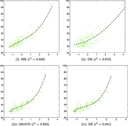
Figure 1: The scatter plot of $Y$ versus $\widehat{\bolds{\beta}}^{\mathrm{T}}\mathbf{x}$, with $\widehat{\bolds{\beta}}$ obtained from SIR, DR, dMAVE and Eff, respectively. The fitted cubic regression curves (–) and the adjusted $\mathrm{r}^{2}$ values are shown.

We calculated the Pearson correlation coefficients and found the current job level ($X_{1}$) has the largest correlation with his/her annual salary ($Y$) [$\operatorname{corr}(X_{1},Y)=0.614$]. This implies that the current job level is possibly an important factor and thus we fix the coefficient of $X_{1}$ to be 1 in our subsequent analysis. We applied SIR, DR, dMAVE and Eff methods to estimate the remaining coefficients. In Figure 1 we present the scatter plots of $Y$ versus a single linear combination $\widehat{\bolds{\beta}}^{\mathrm{T}}\mathbf{x}$, where $\mathbf{x}=(X_{1},\ldots,X_{6})^{\mathrm{T}}$ and $\widehat{\bolds{\beta}}$ denote the estimate obtained from the four estimation procedures. The scatter plots exhibit similar monotone patterns in that the annual salary increases with the value of $\widehat{\bolds{\beta}}^{\mathrm{T}}\mathbf{x}$. Except for DR, the data cloud of all other three proposals looks very compact. To quantify this visual difference, we fit a cubic model by regressing $Y$ on 1, $(\widehat{\bolds{\beta}}^{\mathrm{T}}\mathbf{x}),(\widehat{\bolds{\beta}}^{\mathrm{T}}\mathbf{x})^{2}$ and $(\widehat{\bolds{\beta}}^{\mathrm{T}}\mathbf{x})^{3}$. The adjusted $\mathrm{r}^{2}$ values are also reported in Figure 1. The $\mathrm{r}^{2}$ value of DR is much smaller than that of the other estimators, which suggests worse performance of DR. This is not a surprise because DR requires the most stringent conditions on the covariate vector $\mathbf{x}$, which are violated here because of the categorical covariates. The $\mathrm{r}^{2}$ values of all other estimators including Eff are satisfactory, indicating that $\mathcal{S}_{Y|\mathbf{x}}$ is possibly one dimensional. We would also like to point out that because the $\mathrm{r}^{2}$ value factors in the goodness-of-fit of the cubic model, hence it only provides a reference.

Table 4: The estimated coefficients and standard errors obtained by Eff

		$\bolds{\widehat{\beta}_{2}}$	$\bolds{\widehat{\beta}_{3}}$	$\bolds{\widehat{\beta}_{4}}$	$\bolds{\widehat{\beta}_{5}}$	$\bolds{\widehat{\beta}_{6}}$
Eff	coef.	0.477	0.265	0.024	0.050	0.146
	std.	0.021	0.031	0.030	0.037	0.031
	$p$-value	$<\!10^{-4}$	$<\!10^{-4}$	0.427	0.176	$<\!10^{-4}$

Table 4 contains the estimated coefficients $\widehat{\beta}_{i}$’s, the standard errors and $p$-values obtained through Eff. It can be seen that in addition to the current job level ($X_{1}$), working experience at the current bank ($X_{2}$), age ($X_{3}$) and whether or not the job is computer related ($X_{6}$) are also important factors on salary. While it is not difficult to understand the importance of most of these factors, we believe the age effect is probably caused by its high correlation with the working experience [$\operatorname{corr}(X_{2},X_{3})=0.676$].

6 Discussion

We have derived both locally efficient and efficient estimators which exhaust the entire central subspace without imposing any distributional assumptions. We point out here that if the linearity condition holds, the efficiency bound does not change. However, the linearity condition will enable a simplification of the computation because we can simply plug $E(\mathbf{x}|\bolds{\beta}^{\mathrm{T}}\mathbf{x})=\bolds{\beta}(\bolds{\beta}^{\mathrm{T}}\bolds{\beta})^{-1}\bolds{\beta}^{\mathrm{T}}\mathbf{x}$ into the estimation equation instead of estimating it nonparametrically. However, the constant variance condition does not seem to contribute to the efficiency bound or to the computational simplicity. It is therefore a redundant condition in the efficient estimation of the central subspace.

In this paper we did not discuss how to determine $d$, the structural dimension of $\mathcal{S}_{Y|\mathbf{x}}$ when an efficient estimation procedure is used, although we agree that this is an important issue in the area of dimension reduction. In the real-data example, we infer the structural dimension through the adjusted $\mathrm{r}^{2}$ values. This seems a reasonable choice, but the turnout may depend on how to recover the underlying model structure. How to prescribe a rigorous data-driven procedure is needed in future works.

Various model extensions have been considered in the dimensional reduction literature. For example, in partial dimension reduction problems ChiaromonteCookLi2002 , it is assumed that $F(Y|\mathbf{x})=F(Y|\bolds{\beta}^{\mathrm{T}}\mathbf{x}_{1},\mathbf{x}_{2})$. Here, $\mathbf{x}_{1}$ is a covariate sub-vector of $\mathbf{x}$ that the dimension reduction procedure focuses on, while $\mathbf{x}_{2}$ is a covariate sub-vector that is known to directly enter the model based on scientific understanding or convention. We can see that the semiparametric analysis and the efficient estimation results derived here can be adapted to these models, through changing $\bolds{\beta}^{\mathrm{T}}\mathbf{x}$ to $(\bolds{\beta}^{\mathrm{T}}\mathbf{x}_{1},\mathbf{x}_{2})$ in all the corresponding functions and expectations while everything else remains unchanged. Another extension is the group-wise dimension reduction LiLiZhu2010 , where the model $E(Y|\mathbf{x})=\sum_{i=1}^{k}m_{i}(Y,\mathbf{x}_{i}^{\mathrm{T}}\bolds{\beta}_{i})$ is considered. The semiparametric analysis in such models requires separate investigation, and it will be interesting to study the efficient estimation.

[id=suppA] Supplement to “Efficient estimation in sufficient dimension reduction” [doi]10.1214/12-AOS1072SUPP .pdf aos1072_supp.pdf The supplement file aos1072_supp.pdf is available upon request. It contains derivations of the efficient score for model (1) and an outline of proof for Theorems 1 and 2.

References

- (1) {bbook}[auto:STB—2013/01/23—16:20:06] \bauthor\bsnmAlbright, \bfnmS. C.\binitsS. C., \bauthor\bsnmWinston, \bfnmW. L.\binitsW. L. and \bauthor\bsnmZappe, \bfnmC. J.\binitsC. J. (\byear1999). \btitleData Analysis and Decision Making with Microsoft Excel. \bpublisherDuxbury, \blocationPacific Grove, CA. \bptokimsref \endbibitem
- (2) {bbook}[mr] \bauthor\bsnmBickel, \bfnmPeter J.\binitsP. J., \bauthor\bsnmKlaassen, \bfnmChris A. J.\binitsC. A. J., \bauthor\bsnmRitov, \bfnmYa’acov\binitsY. and \bauthor\bsnmWellner, \bfnmJon A.\binitsJ. A. (\byear1993). \btitleEfficient and Adaptive Estimation for Semiparametric Models. \bpublisherJohns Hopkins Univ. Press, \blocationBaltimore, MD. \bidmr=1245941 \bptokimsref \endbibitem
- (3) {barticle}[mr] \bauthor\bsnmChiaromonte, \bfnmFrancesca\binitsF., \bauthor\bsnmCook, \bfnmR. Dennis\binitsR. D. and \bauthor\bsnmLi, \bfnmBing\binitsB. (\byear2002). \btitleSufficient dimension reduction in regressions with categorical predictors. \bjournalAnn. Statist. \bvolume30 \bpages475–497. \biddoi=10.1214/aos/1021379862, issn=0090-5364, mr=1902896 \bptokimsref \endbibitem
- (4) {barticle}[mr] \bauthor\bsnmCook, \bfnmR. Dennis\binitsR. D. (\byear1994). \btitleOn the interpretation of regression plots. \bjournalJ. Amer. Statist. Assoc. \bvolume89 \bpages177–189. \bidissn=0162-1459, mr=1266295 \bptokimsref \endbibitem
- (5) {bbook}[mr] \bauthor\bsnmCook, \bfnmR. Dennis\binitsR. D. (\byear1998). \btitleRegression Graphics. \bpublisherWiley, \blocationNew York. \biddoi=10.1002/9780470316931, mr=1645673 \bptokimsref \endbibitem
- (6) {barticle}[mr] \bauthor\bsnmCook, \bfnmR. D.\binitsR. D. and \bauthor\bsnmWeisberg, \bfnmS.\binitsS. (\byear1991). \btitleComment on “Sliced inverse regression for dimension reduction,” by K.-C. Li. \bjournalJ. Amer. Statist. Assoc. \bvolume86 \bpages328–332. \bptokimsref \endbibitem
- (7) {barticle}[mr] \bauthor\bsnmDong, \bfnmYuexiao\binitsY. and \bauthor\bsnmLi, \bfnmBing\binitsB. (\byear2010). \btitleDimension reduction for non-elliptically distributed predictors: Second-order methods. \bjournalBiometrika \bvolume97 \bpages279–294. \biddoi=10.1093/biomet/asq016, issn=0006-3444, mr=2650738 \bptokimsref \endbibitem
- (8) {barticle}[mr] \bauthor\bsnmFan, \bfnmJianqing\binitsJ., \bauthor\bsnmYao, \bfnmQiwei\binitsQ. and \bauthor\bsnmTong, \bfnmHowell\binitsH. (\byear1996). \btitleEstimation of conditional densities and sensitivity measures in nonlinear dynamical systems. \bjournalBiometrika \bvolume83 \bpages189–206. \biddoi=10.1093/biomet/83.1.189, issn=0006-3444, mr=1399164 \bptokimsref \endbibitem
- (9) {barticle}[mr] \bauthor\bsnmLi, \bfnmBing\binitsB. and \bauthor\bsnmDong, \bfnmYuexiao\binitsY. (\byear2009). \btitleDimension reduction for nonelliptically distributed predictors. \bjournalAnn. Statist. \bvolume37 \bpages1272–1298. \biddoi=10.1214/08-AOS598, issn=0090-5364, mr=2509074 \bptokimsref \endbibitem
- (10) {barticle}[mr] \bauthor\bsnmLi, \bfnmBing\binitsB. and \bauthor\bsnmWang, \bfnmShaoli\binitsS. (\byear2007). \btitleOn directional regression for dimension reduction. \bjournalJ. Amer. Statist. Assoc. \bvolume102 \bpages997–1008. \biddoi=10.1198/016214507000000536, issn=0162-1459, mr=2354409 \bptokimsref \endbibitem
- (11) {barticle}[mr] \bauthor\bsnmLi, \bfnmBing\binitsB., \bauthor\bsnmZha, \bfnmHongyuan\binitsH. and \bauthor\bsnmChiaromonte, \bfnmFrancesca\binitsF. (\byear2005). \btitleContour regression: A general approach to dimension reduction. \bjournalAnn. Statist. \bvolume33 \bpages1580–1616. \biddoi=10.1214/009053605000000192, issn=0090-5364, mr=2166556 \bptokimsref \endbibitem
- (12) {barticle}[mr] \bauthor\bsnmLi, \bfnmKer-Chau\binitsK.-C. (\byear1991). \btitleSliced inverse regression for dimension reduction (with discussion). \bjournalJ. Amer. Statist. Assoc. \bvolume86 \bpages316–342. \bidissn=0162-1459, mr=1137117 \bptokimsref \endbibitem
- (13) {barticle}[mr] \bauthor\bsnmLi, \bfnmKer-Chau\binitsK.-C. and \bauthor\bsnmDuan, \bfnmNaihua\binitsN. (\byear1989). \btitleRegression analysis under link violation. \bjournalAnn. Statist. \bvolume17 \bpages1009–1052. \biddoi=10.1214/aos/1176347254, issn=0090-5364, mr=1015136 \bptnotecheck year\bptokimsref \endbibitem
- (14) {barticle}[mr] \bauthor\bsnmLi, \bfnmLexin\binitsL., \bauthor\bsnmLi, \bfnmBing\binitsB. and \bauthor\bsnmZhu, \bfnmLi-Xing\binitsL.-X. (\byear2010). \btitleGroupwise dimension reduction. \bjournalJ. Amer. Statist. Assoc. \bvolume105 \bpages1188–1201. \biddoi=10.1198/jasa.2010.tm09643, issn=0162-1459, mr=2752614 \bptokimsref \endbibitem
- (15) {barticle}[mr] \bauthor\bsnmMa, \bfnmYanyuan\binitsY. and \bauthor\bsnmCarroll, \bfnmRaymond J.\binitsR. J. (\byear2006). \btitleLocally efficient estimators for semiparametric models with measurement error. \bjournalJ. Amer. Statist. Assoc. \bvolume101 \bpages1465–1474. \biddoi=10.1198/016214506000000519, issn=0162-1459, mr=2279472 \bptokimsref \endbibitem
- (16) {barticle}[mr] \bauthor\bsnmMa, \bfnmYanyuan\binitsY., \bauthor\bsnmChiou, \bfnmJeng-Min\binitsJ.-M. and \bauthor\bsnmWang, \bfnmNaisyin\binitsN. (\byear2006). \btitleEfficient semiparametric estimator for heteroscedastic partially linear models. \bjournalBiometrika \bvolume93 \bpages75–84. \biddoi=10.1093/biomet/93.1.75, issn=0006-3444, mr=2277741 \bptokimsref \endbibitem
- (17) {barticle}[mr] \bauthor\bsnmMa, \bfnmYanyuan\binitsY. and \bauthor\bsnmGenton, \bfnmMarc G.\binitsM. G. (\byear2010). \btitleExplicit estimating equations for semiparametric generalized linear latent variable models. \bjournalJ. R. Stat. Soc. Ser. B Stat. Methodol. \bvolume72 \bpages475–495. \biddoi=10.1111/j.1467-9868.2010.00741.x, issn=1369-7412, mr=2758524 \bptokimsref \endbibitem
- (18) {barticle}[mr] \bauthor\bsnmMa, \bfnmYanyuan\binitsY., \bauthor\bsnmGenton, \bfnmMarc G.\binitsM. G. and \bauthor\bsnmTsiatis, \bfnmAnastasios A.\binitsA. A. (\byear2005). \btitleLocally efficient semiparametric estimators for generalized skew-elliptical distributions. \bjournalJ. Amer. Statist. Assoc. \bvolume100 \bpages980–989. \biddoi=10.1198/016214505000000079, issn=0162-1459, mr=2201024 \bptokimsref \endbibitem
- (19) {barticle}[mr] \bauthor\bsnmMa, \bfnmYanyuan\binitsY. and \bauthor\bsnmHart, \bfnmJeffrey D.\binitsJ. D. (\byear2007). \btitleConstrained local likelihood estimators for semiparametric skew-normal distributions. \bjournalBiometrika \bvolume94 \bpages119–134. \biddoi=10.1093/biomet/asm020, issn=0006-3444, mr=2307902 \bptokimsref \endbibitem
- (20) {barticle}[mr] \bauthor\bsnmMa, \bfnmYanyuan\binitsY. and \bauthor\bsnmZhu, \bfnmLiping\binitsL. (\byear2012). \btitleA semiparametric approach to dimension reduction. \bjournalJ. Amer. Statist. Assoc. \bvolume107 \bpages168–179. \biddoi=10.1080/01621459.2011.646925, issn=0162-1459, mr=2949349 \bptokimsref \endbibitem
- (21) {bmisc}[auto] \bauthor\bsnmMa, \bfnmYanyuan\binitsY. and \bauthor\bsnmZhu, \bfnmLiping\binitsL. (\byear2013). \bhowpublishedSupplement to “Efficient estimation in sufficient dimension reduction.” DOI:\doiurl10.1214/12-AOS1072SUPP. \bptokimsref \endbibitem
- (22) {barticle}[auto:STB—2013/01/23—16:20:06] \bauthor\bsnmNewey, \bfnmW.\binitsW. (\byear1990). \btitleSemiparametric efficiency bounds. \bjournalJ. Appl. Econometrics \bvolume5 \bpages99–135. \bptokimsref \endbibitem
- (23) {barticle}[mr] \bauthor\bsnmRobins, \bfnmJames M.\binitsJ. M., \bauthor\bsnmRotnitzky, \bfnmAndrea\binitsA. and \bauthor\bsnmZhao, \bfnmLue Ping\binitsL. P. (\byear1994). \btitleEstimation of regression coefficients when some regressors are not always observed. \bjournalJ. Amer. Statist. Assoc. \bvolume89 \bpages846–866. \bidissn=0162-1459, mr=1294730 \bptokimsref \endbibitem
- (24) {bbook}[mr] \bauthor\bsnmTsiatis, \bfnmAnastasios A.\binitsA. A. (\byear2006). \btitleSemiparametric Theory and Missing Data. \bpublisherSpringer, \blocationNew York. \bidmr=2233926 \bptokimsref \endbibitem
- (25) {barticle}[mr] \bauthor\bsnmTsiatis, \bfnmAnastasios A.\binitsA. A. and \bauthor\bsnmMa, \bfnmYanyuan\binitsY. (\byear2004). \btitleLocally efficient semiparametric estimators for functional measurement error models. \bjournalBiometrika \bvolume91 \bpages835–848. \biddoi=10.1093/biomet/91.4.835, issn=0006-3444, mr=2126036 \bptokimsref \endbibitem
- (26) {barticle}[mr] \bauthor\bsnmXia, \bfnmYingcun\binitsY. (\byear2007). \btitleA constructive approach to the estimation of dimension reduction directions. \bjournalAnn. Statist. \bvolume35 \bpages2654–2690. \biddoi=10.1214/009053607000000352, issn=0090-5364, mr=2382662 \bptokimsref \endbibitem
- (27) {barticle}[auto:STB—2013/01/23—16:20:06] \bauthor\bsnmZeng, \bfnmD.\binitsD. and \bauthor\bsnmLin, \bfnmD. Y.\binitsD. Y. (\byear2007). \btitleEfficient estimation in the accelerated failure time model. \bjournalJ. Amer. Statist. Assoc. \bvolume102 \bpages1387–1396. \bptokimsref \endbibitem
- (28) {barticle}[auto:STB—2013/01/23—16:20:06] \bauthor\bsnmZeng, \bfnmD.\binitsD. and \bauthor\bsnmLin, \bfnmD. Y.\binitsD. Y. (\byear2007). \btitleMaximum likelihood estimation in semiparametric models with censored data (with discussion). \bjournalJ. Roy. Statist. Soc. Ser. B \bvolume69 \bpages507–564. \bptokimsref \endbibitem
- (29) {barticle}[mr] \bauthor\bsnmZhu, \bfnmLi-Ping\binitsL.-P., \bauthor\bsnmZhu, \bfnmLi-Xing\binitsL.-X. and \bauthor\bsnmFeng, \bfnmZheng-Hui\binitsZ.-H. (\byear2010). \btitleDimension reduction in regressions through cumulative slicing estimation. \bjournalJ. Amer. Statist. Assoc. \bvolume105 \bpages1455–1466. \biddoi=10.1198/jasa.2010.tm09666, issn=0162-1459, mr=2796563 \bptokimsref \endbibitem
- (30) {barticle}[mr] \bauthor\bsnmZhu, \bfnmYu\binitsY. and \bauthor\bsnmZeng, \bfnmPeng\binitsP. (\byear2006). \btitleFourier methods for estimating the central subspace and the central mean subspace in regression. \bjournalJ. Amer. Statist. Assoc. \bvolume101 \bpages1638–1651. \biddoi=10.1198/016214506000000140, issn=0162-1459, mr=2279485 \bptokimsref \endbibitem