Non-specular reflections in a macroscopic system with wave-particle duality: spiral waves in bounded media.

Abstract

Spiral waves in excitable media possess both wave-like and particle-like properties. When resonantly forced (forced at the spiral rotation frequency) spiral cores travel along straight trajectories, but may reflect from medium boundaries. Here, numerical simulations are used to study reflections from two types of boundaries. The first is a no-flux boundary which waves cannot cross, while the second is a step change in the medium excitability which waves do cross. Both small-core and large-core spirals are investigated. The predominant feature in all cases is that the reflected angle varies very little with incident angle for large ranges of incident angles. Comparisons are made to the theory of Biktashev and Holden. Large-core spirals exhibit other phenomena such as binding to boundaries. The dynamics of multiple reflections is briefly considered.

Wave-particle duality is typically associated with quantum mechanical systems. However, in recent years it has been observed that some macroscopic systems commonly studied in the context of pattern formation also exhibit wave-particle duality. Two systems in particular have attracted considerable attention in this regard: drops bouncing on the surface of a vibrated liquid layer Couder et al. (2005a, b); Protière, Boudaoud, and Couder (2006); Couder and Fort (2006); Eddi et al. (2009a, b) and waves in chemical media Biktasheva and Biktashev (2003); Biktashev (2007); Sakurai et al. (2002); Steele, Tinsley, and Showalter (2008); Biktasheva et al. (2010); Biktashev, Barkley, and Biktasheva (2010). The second case is the focus of this paper. We explore non-specular reflections associated with spiral waves in excitable media – reflections not of the waves themselves, but of the particle-like trajectories tied to these waves.

I Introduction

Rotating spirals are a pervasive feature of two-dimensional excitable media, such as the Belousov-Zhabotinsky reaction Belousov (1959); Zhabotinsky (1964); Zaikin and Zhabotinsky (1970); Winfree (1984). Figure 1(a) illustrates a spiral wave from a standard model of excitable media discussed below. The wave character of the system is evident. As the spiral rotates, a periodic train of excitation is generated which propagates outward from the center, or core, of the spiral. Much of the historical study of excitable media has focused on the wave character of the problem, as illustrated by efforts to determine the selection of the spiral shape and rotation frequency Tyson and Keener (1988); Karma (1991); Bernoff (1991); Margerit and Barkley (2001, 2002).

However, it is now understood that these spiral waves also have particle-like properties. This was first brought to the forefront by Biktasheva and Biktashev Biktasheva and Biktashev (2003) and has been developed in more recent years Biktashev (2007); Biktasheva et al. (2010); Biktashev, Barkley, and Biktasheva (2010); Biktasheva et al. (2009); Biktashev, Biktasheva, and Sarvazyan (2011). One of the more striking illustrations of a particle-like property is resonant drift Agladze, Davydov, and Mikhailov (1987); Davydov et al. (1988); Biktashev and Holden (1993, 1995); Steinbock, Zykov, and Müller (1993); Schrader, Braune, and Engel (1995); Mantel and Barkley (1996); Zhang et al. (2004); Biktashev (2007); Biktasheva et al. (2010), shown in Fig. 1(b)-(d). Resonant drift can occur spontaneously through instability, or due to spatial inhomogeneity, or as here, by means of resonant parametric forcing (periodically varying the medium parameters in resonance with the spiral rotation frequency). As is seen, the core of the spiral drifts along a straight line. The speed is dictated by the forcing amplitude while the direction is set by the phase of the forcing, or equivalently the initial spiral orientation.

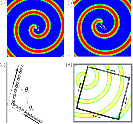
Figure 1: Illustration of resonant drift and reflection for spiral waves in excitable media. (a) Periodically rotating spiral wave in the unforced regime. The wave rotates around a fixed core and the path of the spiral tip (white) is a circle. (b) Resonant drift. The medium is parametrically forced at the spiral rotation frequency. The core moves along a straight path and the spiral tip traces out a cycloid (white). (c) Reflection of drifting spiral from a no-flux boundary. The incident and reflected angles, $\theta_{i}$ and $\theta_{r}$, are indicated. (d) Path of a drifting spiral in a square box. The underlying spiral wave at one instant in time is shown faintly. In all cases the plotted fields are the excitation variable, $u$, of the reaction diffusion model. Details are given later in the text.

The trajectories of drifting spirals are unaffected by the domain boundaries (or other spirals should they be present) except on close approach, where often the result is a reflection of the drifting core Biktashev and Holden (1993, 1995); Olmos and Shizgal (2008), as illustrated in Fig. 1(c). Reflections are not specular – the reflected angle $\theta_{r}$ is not in general equal to the incident angle $\theta_{i}$. When placed in a square box, the drift trajectory typically will ricochet off each boundary in such a way to eventually be attracted to a unique square path where $\theta_{i}+\theta_{r}=90^{\circ}$, as shown in figure 1(d). (This is the more common case, but others are considered herein.)

The primary goal of this paper is firstly to determine accurately, through numerical simulations, the relationship between reflected and incident angles for some representative cases of spiral waves in excitable media, and secondly to explore the qualitative features of reflections in excitable media, particularly multiple reflections in square domains. While the numerical and theoretical study of reflecting trajectories was undertaken by Biktashev and Holden many years ago Biktashev and Holden (1993, 1995), much more extensive results are now possible and desirable, especially since phenomena strikingly similar to that seen in Figs. 1(c) and (d) have been observed in other macroscopic systems with both wave-like and particle-like properties Protière, Boudaoud, and Couder (2006); Eddi et al. (2009b); Sakurai et al. (2002); Steele, Tinsley, and Showalter (2008); Prati et al. (2011); Showalter (2012).

II Model and Methods

Our study is based on the standard Barkley model describing a generic excitable medium Barkley (1991). In the simplest form the model is given by the reaction-diffusion equations

$$\frac{\partial u}{\partial t}=\nabla^{2}u+\frac{1}{\epsilon}u(1-u)\left(u-\frac{v+b}{a}\right),$$ (1)

$$\frac{\partial v}{\partial t}=u-v,$$ (2)

where $u(x,y)$ is the excitation field (plotted in Fig. 1) and $v(x,y)$ is the recovery field; $a$, $b$, and $\epsilon$ are parameters. The parameters $a$ and $b$ collectively control the threshold for and duration of excitation while the parameter $\epsilon$ controls the excitability of the medium by setting the fast timescale of excitation relative to the timescale of recovery.

We consider two parameter regimes – known commonly as the small-core and large-core regimes. The small-core case is shown in Fig. 1. As the name implies, the core region of the spiral, where the medium remains unexcited over one rotation period, is small. This is the more generic case for the Barkley model and similar models and occupies a relatively large region of parameter space in which waves rotate periodically. Small-core spirals are found in the lower right part of the standard two-parameter phase diagram for the Barkley model (see figure 4 of Ref. Barkley, 2008). Large-core spirals rotate around relatively large regions [see Fig. 8(a) discussed below]. Such spirals occur in a narrow region of parameter space Barkley (2008, 1994) near the boundary for propagation failure. The core size diverges to infinity near propagation failure.

Parametric forcing is introduced through periodic variation in the excitability. Specifically we vary $\epsilon$ according to

$$\epsilon(t)=\epsilon_{0}\left(1+A\sin(\omega_{f}t+\phi)\right),$$ (3)

where $A$ and $\omega_{f}$ are the forcing amplitude and frequency. The phase $\phi$ is used to control the direction of resonant drift. The forcing frequency producing resonant drift will be close to the natural, unforced, spiral frequency. However, due to nonlinearity, there is a change in the spiral rotation frequency under forcing and so $\omega_{f}$ must be adjusted with $A$ to produce resonant drift along a straight line.

We have studied reflections in two situations. The first is reflection from a no-flux boundary. This type of boundary condition corresponds to the wall of a container containing the medium. We set the reflection boundary to be at $x=0$ and impose a homogeneous Neumann boundary condition there:

$$\frac{\partial u}{\partial x}(0,y)=0.$$ (4)

Since there is no diffusion of the slow variable, no boundary condition is required on $v$. The medium does not exist for $x<0$.

The second situation we have studied is reflections from a step change in excitability across a line within the medium. We locate step change on the line $x=0$. We vary the threshold for excitation across this line by having the parameter $b$ vary according to

$$b(x,y)=\begin{cases}b_{0}&\text{if $x\geq 0$}\\ b_{0}-\triangle b&\text{if $x<0$}\end{cases}$$ (5)

Unlike for the no-flux boundary, in this case waves may cross the line $x=0$ and so there is no boundary to wave propagation. Nevertheless, drifting spirals may reflect from this step change in the medium and we refer to this a step boundary.

The numerical methods for solving the reaction-diffusion equations are standard and are covered elsewhere Barkley (1991); Dowle, Mantel, and Barkley (1997). Some relevant computational details particular to this study of spiral reflections are as follows. A converged spiral for the unforced system is used as the initial condition. Simulations are started with parametric forcing and the spiral drifts in a particular direction dictated by the phase $\phi$ in Eq. (3). The position of the spiral tip is sampled once per forcing period and from this the direction of drift, i.e. the incident angle $\theta_{i}$, is determined by a least-squares fit over an appropriate range of drift (after the initial spiral has equilibrated to a state of constant drift, both in speed and direction, but before the spiral core encounters a boundary). Likewise, from a fit to the sampled tip path after the interaction with the boundary, we determine the reflected angle $\theta_{r}$. By varying $\phi$ we are able to scan over incident angles.

The simulations are carried out in a large rectangular domain with no-flux boundary conditions on all sides. For reflections from a Neumann boundary (4), we simply direct waves to the computational domain boundary corresponding to $x=0$. We also study reflections more globally from all sides of a square domain with Neumann boundary conditions, such as in Fig. 1(d). In the study of reflections from the step boundary (5), the computational domain extends past the step change in parameter. We have run cases with the left computational boundary both at $x=-7.5$ and $x=-15$ and these are sufficiently far from $x=0$ that trajectory reflection is not affected by the computational domain boundary. The dimensions of the rectangular computational domain are varied depending on the angle of incidence. For $\theta_{i}\simeq\pm 90^{\circ}$ we require a long domain in the $y$-direction, whereas for $\theta_{i}\simeq 0^{\circ}$ a much smaller domain may be used. In all cases we use a grid spacing of $h=1/4$. The time step is varied to evenly divide the forcing period, but $\triangle t\simeq 0.019$ is typical. Except where stated otherwise, the model parameters for the small-core case are: $a=0.8,b=0.05$, and $\epsilon_{0}=0.02$. For the large-core case they are $a=0.6,b=0.07$, and $\epsilon_{0}=0.02$. For the step boundary $b_{0}=0.05$ and $\triangle b=0.025$. Different values of the forcing amplitude and period, $A$ and $\omega_{f}$, are considered. Given the desire to measure incident and reflected angles precisely, we have required drift be along straight lines to high precision and in turn this has required high accuracy in the imposed forcing amplitude and period. In the appendix we report the exact values for the forcing parameters used in the quantitative incidence-reflection studies.

III Results

Before presenting results from our study of reflections, it is important to be precise about the meaning of incident and reflected angles. As is standard, angles are measured with respect to the boundary normal. This is illustrated in Fig. 1(c). What needs to be stressed here is that spirals have a chirality – right or left handedness – and this implies that we need to work with angles potentially in the range $[-90^{\circ},90^{\circ}]$, rather than simply $[0^{\circ},90^{\circ}]$.

Specifically, we consider clockwise rotating spirals and define $\theta_{i}$ to be positive in the clockwise direction from the normal. We define $\theta_{r}$ to be positive in the counterclockwise direction from the normal. Both $\theta_{i}$ and $\theta_{r}$ are positive in Fig. 1(c) and for specular reflections $\theta_{r}=\theta_{i}$.

III.1 Small-core case

We begin with the small-core case already shown in Fig. 1. Figures 2 and 3 illustrate the typical behavior we find in reflections from both types of boundaries. In both figures the upper plot shows measured reflected angle $\theta_{r}$ as a function of incident angle $\theta_{i}$ over the full range of incident angles. The lower plots show representative trajectories for specific incident angles indicated. Here and throughout, the no-flux nature of the Neumann boundary is indicated with shading ($x=0$ is the at the rightmost edge of the shading), while the step in excitability at a step boundary is indicated with sharp lines. All parameters are the same for the two cases; they differ only in the type of boundary that trajectories reflect from.

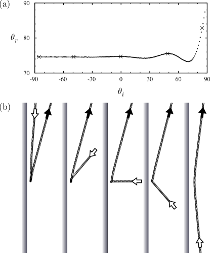
Figure 2: Illustrative results for reflection from a no-flux boundary, i.e. Neumann boundary condition. (a) Reflected angle $\theta_{r}$ versus incident angle $\theta_{i}$. (b) Representative tip trajectories showing reflections at the incident angles marked with crosses in (a). The reflected angle is nearly constant for the full range of incident angles. The forcing amplitude is $A=0.072$.

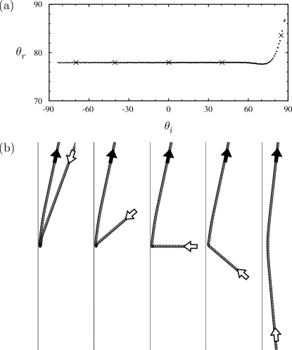
Figure 3: Illustrative results for reflection from a step boundary, i.e. a step change in the excitability of the medium. (a) Reflected angle $\theta_{r}$ versus incident angle $\theta_{i}$. (b) Representative tip trajectories showing reflections at the incident angles marked with crosses in (a). The reflected angle is nearly constant for the full range of incident angles. The forcing amplitude is $A=0.072$.

The reflections are far from specular. This is particularly striking for $\theta_{i}<0$ where the incoming and outgoing trajectories lie on the same side of the normal. The reflected angle is nearly constant, independent of the incident angle, except for incident angles close to $\theta_{i}=90^{\circ}$. There is a slight variation in the reflected angle, seen as undulation in the upper plots, but the amplitude of the variation is small.

One can also observe in the lower plots that the point of closest approach is also essentially independent of incident angle, except close to $\theta_{i}=90^{\circ}$ where the distance grows. Spiral trajectories come much closer to the step boundary than to the Neumann boundary.

It is worth emphasizing that there is no effect of forcing phase in the results presented in Figs. 2 and 3. As the incident angle is scanned, the phase of the spiral as it comes into interaction with the boundaries will be different for different incident angles. While this could have an effect on the reflected angle, we have verified that there is no such effect for the small-core cases we have studied, except at large forcing amplitudes near where spirals annihilate at the boundary (discussed later).

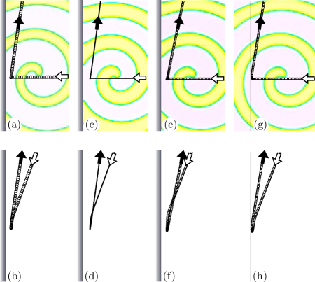
Figure 4: Illustration of the insensitivity of reflections throughout the small-core region of parameter space. Upper plots show $\theta_{i}\approx 0^{\circ}$, including faint visualization of the $u$-field at a particular time instance, while lower plots show $\theta_{i}\approx-70^{\circ}$. The reflected angle is nearly constant independently of incident angle, parameter values, and boundary type. Model parameters span a substantial range of the non-meandering small-core region: in (a) and (b) $a=0.7,b=0.01$; in (c) and (d) $a=0.95,b=0.01$; in (e)-(h) $a=0.95,b=0.08$. Cases (g) and (h) are step boundary, the others are all Neumann boundaries. $A=0.072$ throughout.

While we have not conducted detailed studies at other parameter values, we have explored the small-core region of parameter space. Figure 4 shows representative results at distant points within the small-core region. The figure indicates not only a qualitative robustness, but also a quantitative insensitivity to model parameter values throughout the small-core region. In each case the upper plot shows $\theta_{i}\approx 0^{\circ}$ while the lower plot shows $\theta_{i}\approx-70^{\circ}$. The reflected angle varies by only a few degrees throughout all cases shown in the figure. Case (a)-(b) is close to the meander boundary while (c)-(d) is far from the meander boundary and corresponds to a very small core. Cases (e)-(h) are relatively large values of parameters $a$ and $b$, both with Neumann and step boundary conditions.

In the step boundary case, there is also the effect of $\triangle b$ to consider. Across a number of representative incident angles, we observed that as $\triangle b$ is incremented from $0.025$ up to $0.05$, the closest approaches of the spiral tips occur further from the boundary. We also find a slight reduction in the angle of reflection. Decrementing $\triangle b$ has the opposite effect. However, if $\triangle b$ is too small then the repulsive effect at the boundary will be too small and spiral cores will cross the boundary.

We have examined the effect of forcing amplitude $A$. Figures 5 and 6 show reflected angle as a function of incident angle for various values $A$ as indicated. There is a decrease in the reflected angle with increasing forcing amplitude, or equivalently increasing drift speed. Generally there is also an increase in the oscillations seen in the dependence of reflected angle on incident angle. The solid curves are from the Biktashev-Holden theory discussed in Sec. IV.1.

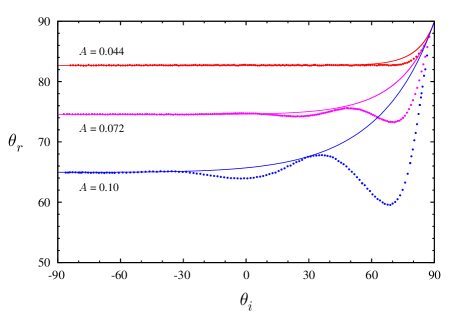
Figure 5: Effect of forcing amplitude on reflection of small-core spirals for the case of a Neumann boundary. Points are measured reflected angle as function of incident angle at forcing amplitudes $A$ indicated. Solid curves are from Biktashev-Holden theory discussed in Sec. IV.1.

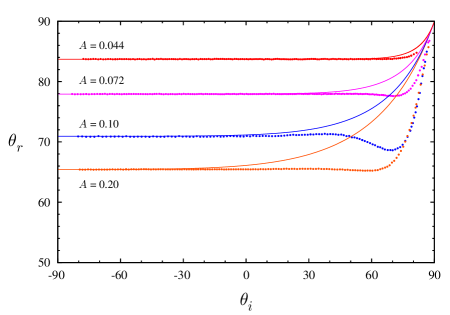
Figure 6: Effect of forcing amplitude on reflection of small-core spirals for the case of a step boundary. Points are measured reflected angle as function of incident angle at forcing amplitudes $A$ indicated. Solid curves are from Biktashev-Holden theory discussed in Sec. IV.1.

For sufficiently large forcing amplitudes small-core spirals may be annihilated as they drift into Neumann boundaries. In such cases no reflection occurs. We have not investigated this in detail as it is outside the main focus of our study on reflections. Nevertheless, we have examined the effect of increasing the forcing amplitude through the point of annihilation for the case of a fixed incident angle $\theta_{i}=0^{\circ}$. The results are summarized in figure 7. The reflected angle reaches a minimum for $A\simeq 0.11$, and thereafter increases slightly, but does not vary by more than $4^{\circ}$ up to the amplitude where annihilation occurs, $A\approx 0.225$, as indicated in figure 7(a). The forcing amplitude at which annihilation first occurs is rather large in that it corresponds to displacing the spiral considerably more than one unforced core diameter per forcing period. Figure 7(b) shows tip trajectories on either side of the amplitude where annihilation occurs, while figure 7(c) shows annihilation at much larger forcing amplitude. We note that the exact amplitude at which annihilation first occurs depends slightly on the rotational phase of the spiral as it approaches the boundary. (Annihilation first occurs in the range $0.22\lesssim A\lesssim 0.23$ depending on phase.) Likewise, the spiral phase can affect the reflected angle by nearly $1^{\circ}$ for $A\gtrsim 0.16$. The influence of phase is nevertheless small for the small-core spirals. It is, however, more pronounced in the large-core case which we shall now discuss.

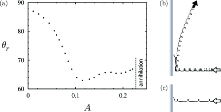
Figure 7: (a) Reflected angle as a function of forcing amplitude $A$ up to the point of annihilation at a Neumann boundary for small-core spirals. The incident angle is fixed at $\theta_{i}=0^{\circ}$. (b) Tip trajectories a little below ($A=0.215$) and a little above ($A=0.235$) the forcing amplitude resulting in annihilation of the spiral at the boundary. (c) Tip trajectory at $A=0.05$ showing annihilation at very large forcing amplitude.

III.2 Large-core case

We now turn to the case where unforced spirals rotate around a relatively large core region of unexcited medium. This case is illustrated in Fig. 8(a) where a rotating spiral wave and corresponding tip trajectory are shown in a region of space the same size as in Fig. 1. The larger tip orbit and unexcited core, as well as the longer spiral wavelength, in comparison with those of Fig. 1(a) are clearly evident. While such spirals occupy a relatively narrow region of parameter space, they are nevertheless of some interest because asymptotic treatments have some success in this region Mikhailov, Davydov, and Zykov (1994); Hakim and Karma (1999) and because this is nearly the same region of parameter space where wave-segments studies are performed Sakurai et al. (2002); Zykov and Showalter (2005); Steele, Tinsley, and Showalter (2008).

Figure 8(b) shows a typical case of non-specular reflection for a large-core spiral compared with a small-core spiral forced at the same amplitude. While many features are the same for the two cases, large-core spirals are found often to reflect at smaller $\theta_{r}$ and moreover, they can exhibit different qualitative phenomena.

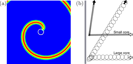
Figure 8: Illustration of a large-core spiral wave. (a) A portion of a rotating spiral and corresponding tip trajectory in a square region $40\times 40$ space units [same size as Fig. 1(a)]. (b) Resonant forcing and reflection for a large-core spiral shown in comparison to that of a small-core spiral. The forcing amplitude is $A=0.05$ in both cases.

Figures 9 and 10 summarize our findings for large-core spirals. Reflected angle as a function of incident angle for three forcing amplitudes is shown in Fig. 9. One sees the overall feature, as with the small-core case, that reflected angle is approximately constant over a large range of incident angles. This is particularly true of low-amplitude forcing, $A=0.022$. However, there are also considerable differences with the small-core case.

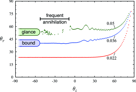
Figure 9: Summary of results for large-core spirals. Reflected angle is plotted versus incident angle for three forcing amplitudes as labeled. Neumann boundary conditions are used. For $A=0.05$ spirals are frequently annihilated at the boundary, [Fig. 10(d)], over the range of incident angles indicated. For $A=0.05$ and $\theta_{i}\lesssim-52^{\circ}$ trajectories glance from the boundary [Fig. 10(a)]. For $A=0.036$ and $\theta_{i}\lesssim-52^{\circ}$ trajectories become bound to the boundary. [See text and Fig. 10(b).] Wiggles are the effect of incident phase.

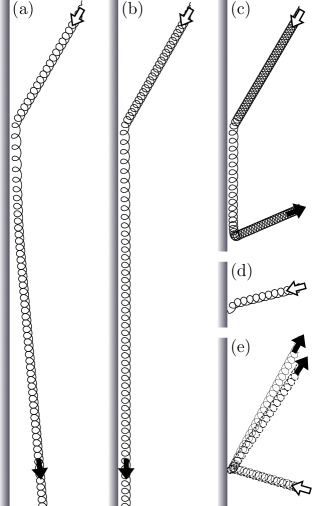
Figure 10: Catalog of interesting trajectories for large-core spirals. (a)-(c) show impacts with $\theta_{i}\approx-60^{\circ}$ at different forcing amplitudes. (a) With $A=0.05$ the trajectory glances from the boundary and moves off nearly parallel to it ($\theta_{r}\approx-85^{\circ}$). (b) With lower amplitude $A=0.036$, the trajectory becomes bound to the boundary. (c) With yet lower amplitude $A=0.022$, the trajectory hugs the boundary for a while then leaves abruptly at an oblique angle ($\theta_{r}\approx 23^{\circ}$). In (d) the incoming spiral with large forcing, $A=0.05$, is annihilated at the boundary. In (e) the effect of phase is seen with two approaching trajectories shifted by half a core diameter. Otherwise the conditions are identical, $A=0.05$. The resulting reflected angles differ slightly.

For large-core spirals the reflected angle increases with forcing amplitude. This is opposite to what is found for small-core spirals in Figs. 5 and 6. Moreover, the reflected angles are noticeably smaller than for the small-core case, as was already observed in Fig. 8(b).

We now focus in more detail on what happens in various circumstances. The left portion of Fig. 9 indicates the different dynamics we observe, depending on forcing amplitude, at large negative incident angles ($\theta_{i}\lesssim-52^{\circ}$), and Figs. 10(a)-10(c) show representative trajectories with $\theta_{i}\approx-60^{\circ}$. At $A=0.05$ trajectories glance off the boundary. That is, they remain close for short while before moving off with a well defined large negative reflected angle. The reflected angle is nearly constant at $\theta_{r}\approx-85^{\circ}$ for incident angles $\theta_{i}\lesssim-52^{\circ}$. At $A=0.036$, $\theta_{i}\lesssim-52^{\circ}$, trajectories become bound to the boundary and move parallel to it indefinitely. In Fig. 10(c), with $A=0.022$, one observes the trajectory moving along the boundary for a distance before abruptly leaving the boundary at a well-defined, relatively small positive reflected angle. This behavior is not restricted to $\theta_{i}\lesssim-52^{\circ}$ and is observed until $\theta_{i}\approx+20^{\circ}$. In fact, this type of reflection is also observed for the other two forcing amplitudes studied for $\theta_{i}$ in a range above $-52^{\circ}$. For $A=0.036$ this occurs until $\theta_{i}$ is approximately $-15^{\circ}$, while for $A=0.05$ this is seen only until $\theta_{i}$ is about $-45^{\circ}$.

At the higher forcing amplitudes, as indicated for the case $A=0.05$ in Fig. 9, large-core spirals are frequently annihilated when they come into contact with the boundary. Figure 10(d) shows a typical example. Whether or not a spiral is annihilated depends very much on the spiral phase on close approach to the boundary. The points shown in Fig. 9 with $A=0.05$ are those where the trajectory reflected; the absence of points indicates annihilation. However, these results are for spirals all initiated a certain distance from the boundary. Changing that distance would affect the spiral phase at close approach and hence a different set of points would be obtained. Nevertheless, the marked range of frequent annihilation is indicative of what occurs at this forcing amplitude.

Finally, we address the wiggles in the reflected angle curves in Fig. 9, most evident at large forcing amplitudes. These wiggles are also due to the fact that the phase of spirals on close approach varies with incident angle. Figure 10(e) illustrates how the reflected angle depends on phase by showing two trajectories shifted by half a core diameter. This shifts the spiral phase upon approach to the boundary and results in slightly different reflected angles. Rather than eliminating these wiggles by averaging over various initial spiral distances, we leave them in as an indication of the variability due to this effect. In general, reflections of large-core spirals are much more sensitive to phase than reflections of small-core spirals, and one should understand that the data in Fig. 9 will vary slightly if similar cases are run with spirals initiated at different distances from the boundary.

While we have not studied the step boundary in detail for large-core spirals, we have carried out a cursory investigation for such a boundary with $\triangle b=0.035$. With the exception that there is no annihilation at the step boundary, we observe qualitatively similar behavior to that just presented for the Neumann case. Most notably we find both glancing and bound trajectories.

IV Discussion

IV.1 Biktashev-Holden theory

Many years ago Biktashev and Holden Biktashev and Holden (1993, 1995) carried out a study very similar in spirit to that presented here. Moreover, they understood that a primary cause for the reflection from boundaries was the small changes in spiral rotation frequency occurring as spiral cores came into interaction with boundaries. Based on this they proposed an appealing simple model to describe spiral reflections. The model is based on the assumption that both the instantaneous drift speed normal to the boundary and spiral rotation frequency are affected by interactions with a boundary, with the interactions decreasing exponentially with distance from the boundary. While the actual interactions between spiral and boundaries are now known to be more complex (see below), it is worth investigating what these simple assumptions give. The beauty of the simple model is that it can be solved to obtain a relationship between reflected and incident angles, depending on only a single combination of phenomenological parameters. (They called this combination $\theta$, but we shall call it $p$. They also used different definitions for incident and reflected angles.)

The model naturally predicts large ranges of approximately constant reflected angle depending on the value of $p$. What is nice is that while fitting the individual phenomenological parameters in their model would be difficult, it is also unnecessary. The value of $p$ can be selected to match the plateau value of $\theta_{r}$ observed in numerical simulations. Then the entire relationship between $\theta_{r}$ and $\theta_{i}$ from the theory is uniquely determined.

Curves from the Biktashev-Holden theory are included in Figs. 5 and 6. While there are obvious limitations to the theory, it is nevertheless interesting to see that some of the features are reproduced just from simple considerations. The theory would be expected to work best where the drift speed is small: low amplitude forcing. For the large-core spirals the theory does not apply and so the corresponding curves are not shown in Fig. 9.

We do not intend here to propose a more accurate theory for the reflection of drift trajectories. It is worth emphasizing, however, that in recent years much has been understood about the interaction between spiral waves and various symmetry breaking inhomogeneities Biktasheva et al. (2010); Biktashev, Barkley, and Biktasheva (2010). The key to this understanding has been response functions, which are adjoint fields corresponding to symmetry modes for spirals in homogeneous media Biktasheva and Biktashev (2003); Biktasheva et al. (2009). In principle, one could now obtain rather accurate description of reflections using this approach, at least for cases in which the boundary could be treated as a weak perturbation of a homogeneous medium. This is beyond the scope of the present study and we leave this for future research.

IV.2 Multiple reflections

As noted in the introduction, Fig. 1(d), when placed within a square domain the trajectory of a drifting spiral will typically approach a square, reflecting from each domain boundary such that $\theta_{i}+\theta_{r}=90^{\circ}$. The reasons for this are simple (see for example Prati, et al.Prati et al. (2011)), but a brief analysis is useful, particularly for understanding when square orbits become unstable.

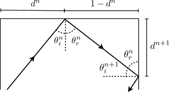
Figure 11: Sketch showing the geometry of multiple reflections in a portion of a square box of normalised length. $d^{n}$ is the location, relative to the length of a side, of the $n^{th}$ reflection.

Figure 11 shows the geometry of a consecutive pair of reflections in the case where the reflected angle is larger than $45^{\circ}$. In this case the path will necessarily strike consecutive sides of the domain. Consider first the path in terms of angles and let $\theta_{i}^{n}$ and $\theta_{r}^{n}$ denote, respectively, the $n^{th}$ incident and reflected angles, starting from the initial reflection $\theta_{i}^{0},\theta_{r}^{0}$. Trivially, the geometry of the square domain dictates that $\theta_{i}^{n+1}+\theta_{r}^{n}=90^{\circ}$. Then, if the trajectory approaches an attracting path with constant angles, $\lim_{n\to\infty}\theta_{i}^{n}=\theta_{i}^{*}$, $\lim_{n\to\infty}\theta_{r}^{n}=\theta_{r}^{*}$, it must be that this path satisfies $\theta_{i}^{*}+\theta_{r}^{*}=90^{\circ}$. That is, it must be a square or a rectangle. Denoting the relationship between incident and reflected angle by $\theta_{r}=\Theta(\theta_{i})$, then a necessary condition for the square path to be attracting is that $|\Theta^{\prime}(\theta_{i}^{*})|<1$. For the cases we have studied this is true since $|\Theta^{\prime}(\theta_{i}^{*})|\simeq 0$.

Turning now to the points at which the path strikes the edge of the domain, we let $d^{n}$ denote the position of the $n^{th}$ reflection along a given side, relative to the length of a side. One can easily see from the geometry that $d^{n+1}=(1-d^{n})\cot\theta_{r}^{n}$. Now, since $\theta_{r}\to\theta_{r}^{*}$, the fixed point $d^{*}$ is given by $d^{*}=(1-d^{*})\cot\theta_{r}^{*}$, or $d^{*}=1/(1+\tan\theta_{r}^{*})$. This corresponds to a square trajectory. For example, from Fig. 5 with a forcing amplitude $A=0.072$ one can see that $\theta_{r}^{*}$ will necessarily be about $74^{\circ}$, giving $d^{*}\approx 0.22$. These are the values seen in the simulation in Fig. 1(d). A necessary condition for this fixed point to be stable is $|\cot\theta_{r}^{*}|<1$. For small-core spirals $\theta_{r}^{*}>45^{\circ}$, so $\cot\theta_{r}^{*}<1$, and hence their square paths are stable.

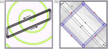
Figure 12: Examples of non-square paths for large-core spirals. (a) $A=0.022$. The reflected angle is considerably smaller than $45^{\circ}$ and the resulting trajectory bounces between opposite sides of the domain. The spiral is shown faintly at one time instance. (b) $A=0.034$. The square trajectory is unstable. For the first circuit around the nearly square path the full tip trajectory is plotted. Subsequently, for clarity only, the tip path sampled once per forcing period is shown. The trajectory collapses towards the diagonal. The final portion of the trajectory before the spiral approaches the corners is shown in bold. The spiral undergoes a complicated reflection from the corner (gray, dotted).

While square trajectories occur for small-core spirals, for large-core spirals other trajectories are possible. Examples are shown in Fig. 12. These occur when the reflected angle is smaller than $45^{\circ}$. (It is possible that $\theta_{r}<45^{\circ}$ might occur for small-core spirals in some regimes, although we have not observed them.) When $\theta_{r}<45^{\circ}$ it is not necessarily the case that trajectories will strike consecutive sides of a square box. This is seen in Fig. 12(a) where the spiral in reflects between opposite sides of the domain. The reflections satisfy $\theta_{r}=-\theta_{i}$.

The more interesting case is when $\theta_{r}$ is only slightly less than $45^{\circ}$ as is seen in Fig. 12(b). The square trajectory is unstable. While $|\Theta^{\prime}(\theta_{i}^{*})|<1$ and the angles converge quickly to $\theta_{i}^{n}+\theta_{r}^{n}\simeq 90^{\circ}$, the equation $d^{n+1}=(1-d^{n})\cot\theta_{r}^{n}$ exhibits growing period-two oscillations for $\cot\theta_{r}^{n}$ slightly larger than 1. Period-two oscillations in $d^{n}$ with $\theta_{i}^{n}+\theta_{r}^{n}\simeq 90^{\circ}$ correspond to approximately rectangular trajectories that approach a diagonal. This ultimately leads the spiral into a corner of the domain where it may reflect in complicated manner.

The analysis just presented should not be viewed as a model for spiral trajectories. Rather it just shows what global dynamics can be deduced simply from a measured relationship between incident and reflected angles. Essentially this same analysis appears as part of a study of cavity solitions Prati et al. (2011) which also undergo non-specular reflections from walls and hence exhibit square orbits similar to figure 1(d). Our simple analysis should be contrasted with the situation for drops bouncing on the surface of an oscillating liquid, so called walkers. Here physical models of the liquid surface and drop bounces account for many varied features of the system Protière, Boudaoud, and Couder (2006); Couder and Fort (2006); Protière, Bohn, and Couder (2008); Fort et al. (2010); Eddi et al. (2011); Shirokoff (2012). The corresponding theory for spiral waves would be that based on response functions in which many details of drift trajectories can be predicted Biktasheva et al. (2010); Biktashev, Barkley, and Biktasheva (2010), although as of yet not reflections from boundaries. Memory effects are important for walkers because bouncing drops interact with surface waves generated many oscillations in the past, and models necessarily take this into account Couder and Fort (2006); Fort et al. (2010); Eddi et al. (2011); Shirokoff (2012). However, path memory is absent from spiral waves in excitable media and this constitutes a significant difference between the two systems.

IV.3 Concluding remarks

We have reported some quantitative and some qualitative features of resonant-drift trajectories in excitable media. The main message is that reflections are far from specular – the reflected angle generally depends only weakly on the incident angle and typically is nearly constant over a substantial range of incident angles (particularly negative incident angles). Biktashev-Holden theory Biktashev and Holden (1993, 1995) accounts for some of the observed features, but a more detailed theory based on response functions Biktasheva and Biktashev (2003); Biktasheva et al. (2010); Biktashev, Barkley, and Biktasheva (2010) is needed. We have seen that the behavior of large-core spirals is more varied than that for small-core ones. Rather than simply reflecting from a boundary, large-core spirals may sometimes become bound to, or glance from, or be annihilated at a boundary, even at moderate forcing amplitudes. Finally we have considered what can occur as spirals undergo multiple reflections within a square domain, and in particular have shown that while small-core spirals are observed to meet the conditions of stable square trajectories, large-core spirals may fail to meet these conditions and exhibit more interesting dynamics.

We motivated this study with a broader discussion of macroscopic systems with wave-particle duality. A large number of analogues to quantum mechanical systems have been reported for walkers on the surface of a vibrated liquid layer Couder et al. (2005a, b); Protière, Boudaoud, and Couder (2006); Couder and Fort (2006); Eddi et al. (2009a, b). As far as we are aware, this is less the case for the propagating wave segments studied by Showalter et al.Sakurai et al. (2002); Zykov and Showalter (2005); Steele, Tinsley, and Showalter (2008) or the drifting spirals in excitable media considered here. (We examined briefly small-core drift trajectories through a single slit, but did not observe diffraction-like behavior.) Nevertheless, for the reflection problem, spiral trajectories, propagating wave segments, cavity solitons, and walkers all share the feature of non-specular reflections Protière, Boudaoud, and Couder (2006); Steele, Tinsley, and Showalter (2008); Prati et al. (2011); Couder and Fort (2012) and as a result these systems can show similar dynamics when undergoing multiple reflections within a bounded region Protière, Boudaoud, and Couder (2006); Eddi et al. (2009b); Steele, Tinsley, and Showalter (2008); Prati et al. (2011); Showalter (2012). It will be of interest to make further quantitative comparisons between these different systems in the future and to explore theoretical basis of this behavior.

Appendix: Forcing parameter values

In the appendix we report the exact values for the forcing parameters used in the detailed quantitative incidence-reflection studies, since obtaining high-precision values for resonant drift can be time consuming. The values stated in the body of the paper are reported only to two significant figures.

Table 1: Parameter values used to produce resonant (straight line) drift in the small-core case ($a=0.8$, $b=0.05$).

$A$	$\omega_{f}$	$\triangle t$
0.044462	1.82	0.0187625
0.071868	1.792	0.0188508
0.102609	1.75	0.0188968
0.196132	1.63	0.0188957

Table 2: Parameter values used to produce resonant (straight line) drift in the large-core case ($a=0.6$, $b=0.07$).

$A$	$\omega_{f}$	$\triangle t$
0.022	1.025	0.0188035
0.035863	1.003	0.0187557
0.050144	0.989	0.0187961