On the development of the Papaloizou-Pringle instability of the black hole-torus systems and quasi-periodic oscillations

Abstract

We present the numerical study of dynamical instability of a pressure-supported relativistic torus, rotating around the black hole with a constant specific angular momentum on a fixed space-time background, in case of perturbation by a matter coming from the outer boundary. Two dimensional hydrodynamical equations are solved at equatorial plane using the HRSCS to study the effect of perturbation on the stable systems. We have found that the perturbed torus creates an instability which causes the gas falling into the black hole in a certain dynamical time. All the models indicate an oscillating torus with certain frequency around their instant equilibrium. The dynamic of the accreted torus varies with the size of initial stable torus, black hole spin and other variables, such as Mach number, sound speed, cusp location of the torus, etc. The mass accretion rate is slightly proportional to the torus-to-hole mass ratio in the black hole-torus system, but it strongly depends on the cusp location of the torus. The cusp located in the equipotential surfaces of the effective potential moves outwards into the torus. The dynamical change of the torus increases the mass accretion rate and triggers the Papaloizou-Pringle instability. It is also observed that the growth of the $m=1$ mode of the Papaloizou-Pringle instability occurs for a wide range of fluid and hydrodynamical parameters and a black hole spin. We have also computed the QPOs from the oscillating relativistic torus.

1 Introduction

The coalescing of compact binaries and their interactions with accretion discs are important issues in astrophysics. The recent review about the black hole accretion disc theory given by Abramowicz & Fragile (2013) explains how the interaction of accretion disc with a black hole reveals predictions of emission, signature of strong gravity, black hole mass, and spin. The merging of BH-BH, BH-NS or NS-NS, or accreting a hot matter rotating around compact objects may cause a torus to be formed which might be responsible for oscillation and emission of BH-torus systems. The hot torus around the black hole is thought to be a mechanism gather the particles and form a jet. The internal shocks inside the jets can create high energy particles and lead to the emission of gamma-ray photons(Meszaros, 2006). It is important to understand the dynamics, formation, and stability properties of a torus to show how the gamma rays are formed.

The rapid destruction of an accretion disc due to high accretion rate, which is larger than the Eddington rate, was first suggested by Abramowicz et.al. (1983). They pointed out that the cusp located in the equipotential surfaces of the effective potential moves outwards into the torus. This physical change in the black hole-torus system can increase the mass accretion rate and mass of the black hole, and it causes a runaway instability. The runaway instability was firstly discovered by (Abramowicz et.al., 1983) using a pseudo-Newtonian potential and studied in relativity by Font & Daigne (2002). The comprehensive study of relativistic thick disk which has a non-constant angular momentum around the black holes has been done by Daigne & Font (2004). They found that the disk is dramatically stabilized in case of very small values of angular momentum slopes. The non-constant angular momentum disk displays more unstable behavior and it causes to grow the mode of the runaway instability more fast. The instability of accreting torus orbiting around the non-rotating black hole was studied by Montero et.al. (2010), and their numerical simulations showed that axisymmetric oscillation of torus was exhibited without the appearance of the runaway instability. It is also indicated that the self gravity of the torus does not play an important role for the occurring of the instability in a few dynamical time steps. Recently, Korobkin et.al. (2013), for the first time, demonstrated the runaway instability for a constant distribution of the specific angular momentum by using the fully self-consistent general relativistic hydrodynamical evolution. They have confirmed that the runaway instability occurred in a few dynamical times.

The Papaloizou-Pringle instability represents the instability of the torus around the compact objects. The origin of the Papaloizou-Pringle instability is mostly related with the interaction between the propagation of waves across the co-rotation radius (Papaloizou & Pringle, 1984). The waves inside the co-rotation radius carry negative energy while the waves outside of this radius carry positive energy. When the waves inside the co-rotation radius lose energy to the waves outside the co-rotation radius, the instability occurs (Blaes & Glatzel, 1986). The Papaloizou-Pringle instability on the torus was studied by a number of authors in literature. The number of physical parameters play a dominant role emerging from the hydrodynamical instabilities occurred as a result of interaction between perturbation and the black hole-torus system. Three-dimensional space parameter of the torus size, the torus angular momentum and angular momentum of the black hole was studied by De Villiers & Hawley (2002). The growth of the Papaloizou-Pringle instability was observed for a range of initial configuration of the black hole-torus system. The effect of magnetic field on the Papaloizou-Pringle instability in the torus was revealed by Fu & Lai (2011) using the various magnetic structures and strengths. They have found that the toroidal magnetic fields affect the Papaloizou-Pringle instability. The self-gravity of the relativistic torus orbiting around the black hole may be thought as a central engine of GRBs. So it is important to understand its dynamic, formation and stability properties. The instabilities of the self-gravitating torus were studied by Kiuchi et.al. (2011); Korobkin et.al. (2013) using the general relativistic hydrodynamics code and they showed that the Papaloizou-Pringle instability grows for a self-gravitating relativistic torus around the black hole.

The interacting matter with a black hole or falling matter into a black hole is a source of gravitation radiation. Perturbation of the torus by matter modifies the fluid around the black hole and shock may be formed. The rotating shock can cause a matter to have a non-linear behavior and its energy heats the gas. So the electromagnetic flares would be produced and these flayers continue to occur for a long time (Schnittman & Krolik, 2008). Interacting particles with shock waves in the equatorial plane produce a continues emission ranging from Ultra-Viole to X-rays if they freely drive away from the black hole-torus system (Rees & Meszaros, 1994).

It is known that the central region of the black hole-disc system, which produces the Gamma Ray Burst (GRB), is not significantly bigger than the size of the black hole. So the torus is a possible physical mechanism to produce GRB and gravitational waves which are used to identify the nature of the inner region that may be observed from GRB system (Kiuchi et.al., 2011). The small perturbations on the torus create a hydrodynamical instability which is responsible for gravitational waves. Its contribution to the gravitational wave background was estimated by Coward et.al. (2002). The gravitational wave radiation from the center of GRB, which consists of a black hole and torus, was studied by Lee (2004). It was found that the gravitational wave is a natural phenomenon in the wobbling system.

Oscillation properties of the black hole-torus system have been studied for numbers of astrophysical systems. Investigating the oscillating system can allow us to expose disco-seismic classes which are dominant in relativistic geometrically thin disc. Some numerical studies revealed the oscillatory modes of the perturbed torus (Zanotti et.al., 2003; Rezzolla et.al., 2003; Montero et.al., 2007). Oscillation properties of the pressure-supported torus were also examined by Schnittman & Rezzolla (2006). They had found a strong correlation between intrinsic frequency of the torus, which is also called the relative frequency and the frequency of oscillation computed from data that is dumped from the mean wind, and extrinsic frequency, which is a frequency recorded by an observer moving with the flow, shown in observed light curve power spectrum. The analysis of Quasi-Periodic Oscillations (QPOs) was motivated by observed data coming from the galactic center, low-mass $X-$ ray binaries (van der Klis, 2004) and high frequency phenomena, testing the strong gravity (Bursa et.al., 2004) in the innermost region of accretion disc around the black hole.

The Observations with X-ray telescopes have uncovered the existing of QPOs of matter around the black holes (Remillard et.al., 1999; Strohmayer, 2001). The QPOs can be used to test the strong gravity and the properties of the black hole since they are originated close to the black hole (Dönmez et.al., 2011; Abramowicz & Fragile, 2013). In order to understand these physical properties, the perturbed pressure-supported torus is examined in a close-binary system. In this paper, our main goal is to study the instability of a stable torus on the equatorial plane based on perturbation, which is coming from the outer boundary of computational domain. In order to do that we solve hydrodynamical equations on a curved fixed space-time for the non-rotating and rotating black holes at the equatorial plane. Thus, we investigate the effects of perturbation and thermodynamical parameters onto the tori’s instability. It is astrophysically possible that a stable black hole-torus system might be perturbed by a blob of gas like observed in $SgrA^{*}$. We have perturbed the torus in a different way from the those used in Montero et.al. (2007); Schnittman & Rezzolla (2006); Zanotti & Rezzolla (2003) in which it was performed by applying a perturbation to the radial velocity of the torus and Zanotti et.al. (2005) in which three different types of perturbations, such as the perturbation of the radial velocity, a small variation of the density of the torus and a linear perturbation of the density and radial velocity, were used.

In this work, we study the effect of perturbation onto the torus-black hole system by solving the hydrodynamical equations on a fixed background space-time. The paper is organized as follows: in section 2, we briefly explain the formulation, numerical setup, boundary and initial condition and introduce the initial setup of the relativistic torus. The numerical results are described in 3. The outcomes of interaction of the torus-black hole system with matter as a result of perturbation coming from the outer boundary and QPOs due to oscillation of the torus are presented Finally, Section 4 concludes our findings. Throughout the paper, we use geometrized unit, $G=c=1$ and space-time signature $(-,+,+,+)$.

2 Equations, Numerical Setups, Boundary and Initial Conditions

2.1 Equations

We consider a non-self gravitating a torus with an equation of state of a perfect fluid in a hydrostatics equilibrium around the non-rotating and rotating black holes. In order to model the instability of the torus due to perturbation, we have solved the hydrodynamical equations on a curved fixed space-time using the equation of state of a perfect fluid. The hydrodynamical equations are

$$\bigtriangledown_{\mu}T^{\mu\nu}=0,\;\;\;\bigtriangledown_{\mu}J^{\mu}=0,$$ (1)

where $T^{\mu\nu}=\rho hu^{\mu}u^{\nu}+Pg^{\mu\nu}$ is a stress-energy tensor for a perfect fluid and $J^{\mu}=\rho u^{\mu}$ is a current density. To preserve and use the conservative properties of hydrodynamical equations, Eq.1 is written in a conservative form using the $3+1$ formalism, and we have (Font et.al., 2000)

$$\frac{\partial{\bf{U}}}{\partial t}+\frac{\partial{\bf{F}}^{r}}{\partial r}+\frac{\partial{\bf{F}}^{\phi}}{\partial\phi}={\bf{S}}\ ,$$ (2)

where $\bf{U}$ is a conserved variable and, $\bf{F}^{r}$ and $\bf{F}^{\phi}$ are fluxes in radial and angular direction at equatorial plane, respectively. These quantities depend on fluid and thermodynamical variables which are written explicitly in detail in Dönmez (2004); Font et.al. (2000). $\bf{S}$ represents the source term which depends on space-time metric $g^{\mu\nu}$, Christoffel symbol $\Gamma^{\alpha}_{\mu\nu}$, lapse function $\alpha$, determinant of three metric $\gamma_{ij}$ and stress-energy tensor $T^{\mu\nu}$. The conserved variables and fluxes also depend on the velocity of fluid and Lorenz factor. The covariant components of three-velocity $v^{i}$ can be defined in terms of four-velocity $u^{\mu}$ as $v^{i}=u^{i}/(\alpha u^{t})$ and Lorenz factor $W=\alpha u^{0}=(1-\gamma_{ij}v^{i}v^{j})^{-1/2}$. The explicit representation of hydrodynamical equations on a curved fixed background space-time and their numerical solutions at equatorial plane are given in Dönmez (2004); Yildiran & Dönmez (2010).

2.2 Numerical Setups and Boundary Conditions

We have solved the hydrodynamics (GRH) equations at the equatorial plane to model the perturbed torus around the black hole. The code used in this paper, which carries out the numerical simulation, was explained in detail by Dönmez (2004); Dönmez et.al. (2011); Yildiran & Dönmez (2010), which gives the solutions of the GRH equations using Marquina method with MUSCL left and right states. Marquina method with MUSCL scheme guarantees higher order accuracy and gives better solution at discontinuities mostly seen close to the black hole. The pressure of the gas is computed by using the standard $\Gamma$ law equation of state for a perfect fluid which defines how the pressure changes with the rest-mass density and internal energy of the gas, $P=(\Gamma-1)\rho\epsilon$ with $\Gamma=4/3$. After setting up the stable torus with a constant specific angular momentum inside the region, $r_{in}<r<r_{max}$, we have to also define the vacuum, the region outside of the $r_{in}<r<r_{max}$ at where all the variables set to some negligible values. We have used the low density atmosphere, $\rho_{atm}=10^{-8}\rho_{c}$, outside of the torus in the computational domain. The other variables of atmosphere are $p_{atm}=10^{-8}p_{c}$, $V^{r}=0.0$ and $V^{\phi}=0.0$. The numerical evolution of torus showed that the dynamic of steady-state torus was unaffected by the presence of the given atmosphere. The Kerr metric in Boyer-Lindquist coordinates is used to set up the black hole at the center of computational domain using an uniformly spaced grid in $r$ and $\phi$ directions. The $r$ goes from $2.8M$ to $200M$ for non-rotating, and $1.7M$ to $200M$ for rotating black holes while $\phi$ varies between $0$ and $2\pi$. Typically, we use $N_{r}$ $X$ $N_{\phi}$ $=$ $3072$ $X$ $256$ zones in radial and angular directions at the equatorial plane.

The boundaries must have been correctly resolved to avoid unwanted oscillations. So we set up an outflow boundary condition at physical boundaries of computation domain in radial direction. All the variables are filled with values using zeroth-order extrapolation. While the velocity of matter, $v^{r}$, must be less than zero at close to the black hole, it should be bigger than zero at the outer boundary of computation domain. The positive radial velocity at the outer boundary lets the gas to fall out from computational domain. So the unwanted oscillations which may arise at the outer boundary can not propagate into the computational domain. The periodic boundary condition is used in angular direction.

2.3 Initial Torus Dynamics

The analytic representation of the non-self-gravitating relativistic torus for a test fluid was first examined by Abramowicz et.al. (1978). They found a sharp cusp for marginally stable accreting disc which was located at an equatorial plane. Later, the torus with an equation of state of a perfect fluid was discussed in detail in Zanotti & Rezzolla (2003); Zanotti et.al. (2003, 2005); Nagar et.al. (2005), numerically. The matter of torus is rotating at a circular orbit with non-geodesic flow between $r_{in}$ and $r_{max}$, and the polytropic equation of state, $P=K\rho^{\Gamma}$, is used to build an initial torus in hydrodynamical equilibrium with the values of variables given in Table 1. Using the $\Gamma=4/3$ , it mimics a degenerate relativistic electron gas. The significant internal pressure in the torus can balance the centrifugal and gravitational forces to maintain the system in hydrodynamical equilibrium.

Some of the astrophysical systems, which have a torus type structure, may be formed as a consequence of the merger of two black holes, two neutron stars, their mixed combination or form in the core collapse of the massive stars. These phenomena suggest that the torus might be in non-equilibrium state after it is formed. In order to understand the physical phenomena of a non-stable black hole torus system and perturbation of the torus by a matter which is coming from the outer boundary of computational domain, we build the initial conditions for a non-self gravitating perfect-fluid torus orbiting around a black hole using the formulations given by Zanotti & Rezzolla (2003); Zanotti et.al. (2003) that assumes to be a non-geodesic motion of the flow . We have considered different initial conditions and perturbations given in Table 1.

Table 1: Initial models of the perturbed torus around the black hole at the equatorial plane. From left to right: $P$ shows the model name, $a$ is the spin parameter of the black hole, $M_{t}/M_{BH}$ is the torus-to-hole mass ratio, $K(geo)$ is the polytropic constant in geometrized unit, $\ell_{0}$ is the constant specific angular momentum, $r_{in}$ and $r_{out}$ are the inner and the outer edges of the torus, $r_{cusp}(M)$ is the cusp location, $\rho_{c}(geo)$ is the density at the center of the torus, $r_{c}(M)$ represents the location at where density is maximum, $t_{orb}(M)$ is the orbital period at $r=r_{c}$, $C_{s}$ and $\mathcal{M}$ are the speed of sound and the Mach number of perturbation, respectively. The total time of the simulations varies depending on models.

											$\bf{Param.}$ $\bf{of}$	$\bf{Perturb.}$
Model	$\frac{a}{M}$	$\frac{M_{t}}{M_{BH}}$	$K(geo)$	$\rho_{c}(geo)$	$\ell_{0}$	$r_{in}$	$r_{out}$	$r_{cusp}(M)$	$r_{c}(M)$	$t_{orb}(M)$	$C_{s}(c)$	$\mathcal{M}$
$P_{1}$	$0.0$	$0.1$	$4.969$ x $10^{-2}$	$7.329$ x $10^{-5}$	$5.44$	$15.0$	$72.99$	$2.91$	$25$	$785.3$	$0.001$	$2$
$P_{2}$	$0.0$	$0.1$	$4.969$ x $10^{-2}$	$7.329$ x $10^{-5}$	$5.44$	$15.0$	$72.99$	$2.91$	$25$	$785.3$	$0.001$	$2$
$P_{3}$	$0.0$	$0.1$	$4.969$ x $10^{-2}$	$1.140$ x $10^{-4}$	$3.80$	$4.57$	$15.889$	$4.57$	$8.35$	$151.6$	$0.001$	$2$
$P_{4}$	$0.0$	$0.1$	$4.969$ x $10^{-2}$	$1.140$ x $10^{-4}$	$3.80$	$4.57$	$15.889$	$4.57$	$8.35$	$151.6$	$0.01$	$2$
$P_{5}$	$0.0$	$0.01$	$3.184$ x $10^{-2}$	$2.863$ x $10^{-6}$	$3.95$	$5.49$	$29.08$	$4.107$	$9.97$	$197.7$	$0.001$	$2$
$P_{6}$	$0.0$	$1$	$2.294$ x $10^{-2}$	$1.153$ x $10^{-3}$	$3.80$	$4.57$	$15.889$	$4.57$	$8.35$	$151.6$	$0.001$	$2$
$P_{7}$	$0.0$	$0.1$	$3.601$ x $10^{-2}$	$1.628$ x $10^{-4}$	$3.784$	$4.64$	$14.367$	$4.64$	$8.16$	$146.4$	$0.001$	$2$
$P_{8}$	$0.0$	$1$	$2.294$ x $10^{-2}$	$1.153$ x $10^{-3}$	$3.80$	$4.57$	$15.889$	$4.57$	$8.35$	$151.6$	$0.001$	$200$
$P_{9}$	$0.0$	$0.1$	$3.601$ x $10^{-2}$	$1.628$ x $10^{-4}$	$3.784$	$4.64$	$14.367$	$4.64$	$8.16$	$146.4$	$0.001$	$0.1$
$P_{10}$	$0.9$	$0.1$	$4.969$ x $10^{-2}$	$1.140$ x $10^{-4}$	$2.60$	$1.78$	$19.25$	$1.78$	$3.40$	$39.4$	$--$	$--$
$P_{11}$	$0.9$	$0.1$	$4.969$ x $10^{-2}$	$1.140$ x $10^{-4}$	$2.60$	$1.78$	$19.25$	$1.78$	$3.40$	$39.4$	$0.001$	$2$
$P_{12}$	$0.9$	$0.05$	$4.969$ x $10^{-2}$	$1.999$ x $10^{-5}$	$3.303$	$-$	$21.23$	$1.41$	$7.40$	$126.5$	$0.001$	$2$

2.4 Astrophysical Motivation

The numerical simulations of the astrophysical systems are getting more popular to understand the dynamics of the systems and to explain the physical phenomena in the results obtained from the observational data. One of the interesting problems in astrophysics is the torus around the black hole. The interaction of torus with a black hole may create instability as a consequence of perturbation. It is believed that the central engine for GRBs is the black hole-torus system. Microquasars also consist of the black holes which are surrounded by the tori (Levinson & Blandford, 1996). The perturbation is one of the mechanism of the evolution triggering the instability in the black hole-torus system to consider the observational and physical results of the torus and the black hole. Upcoming and lunched ground- and space-base detectors will detect high energetic astrophysical phenomena that may be the product of interaction of the black hole-torus system. The possible applications of our results can be used in the phenomena which are offered by a source in microquasars and GRBs. The perturbations of these systems could be consequence of a matter coming from the outer boundary like reported for $Sgr$ $A^{*}$. The component of the gas cloud, falling toward to $Sgr$ $A^{*}$, has been reported by Burkert et.al. (2012). It is seen from this report that the gas cloud is captured and will accreate on $Sgr$ $A^{*}$ and perturb the possible accretion disk, which could be a shock cone (Dönmez et.al., 2011) or torus (Moscibrodzka et.al., 2006), around the black hole in our galactic center. Such a perturbation may explain the properties of the flare emission observed in the innermost part of accretion disk in the center of our galaxy. In addition, the perturbation which has a localized density and is similar to those of a dense stellar wind may help us to understand the internal structure of super-giant fast X-ray transient outbursts.

3 Numerical Results

The numerical results given in this paper are classified depending on the torus-to-black hole mass ratio and black hole spin as well as the size of the pressure-supported stable torus around the black hole. The perturbation will cause to the oscillation and dynamical change of the torus during the evolution.

We adopt the perturbation from the outer boundary at $3.1<\phi<3.18$ between $t=0M$ and $t=80M$ for all models except model $P_{2}$, which has a continues injection during the evolution, with different parameters given in Table 1 and the rest-mass density of perturbation is $\rho_{p}=0.9\rho_{c}$ for all models. The perturbation-to-torus mass ratio is $M_{p}/M_{t}\sim 0.00001$. The matter is injected toward the torus-black hole system with radial velocities, $V^{r}=0.002$, $V^{r}=0.02$, $V^{r}=0.2$, and $V^{r}=0.0001$ and with an angular velocity, $V^{\phi}=0.00001$ for all $V^{r}$, accelerated radially and reached the torus around $t=3000M$. The ratio of angular velocity of the perturbed matter to Keplerian angular velocity is $V^{\phi}/\Omega_{K}=1/35$ at the outer boundary, $r=200M$. We use such a small angular velocity for perturbation due to the technical difficulties. If the perturbing stream carries significant angular momentum, the code crashes due to low values of atmosphere’s parameters. The perturbation which is rotating with a high angular velocity and has a very strong shock could crush the code. While the period of matter at the center of torus is around $T_{c}=151M$ for models $P_{3}$, $P_{4}$, $P_{6}$ and $P_{8}$, it is $T_{c}=785M$ for models $P_{1}$ and $P_{2}$. The perturbation starts to influence the torus after $\sim 16$ orbital period of the torus which has highest density around $r\approx 9M$ for models $P_{3}$, $P_{4}$, $P_{6}$ and $P_{8}$. But it is $\sim 4$ orbital period for models $P_{1}$ and $P_{2}$ given in in Table 1. These orbital periods are measured at the location where the rest-mass density is maximum in the unperturbed torus.

3.1 Perturbed Torus Around the Non-Rotating Black Hole

To analyze the dynamics of the torus and its instability after the perturbation, we plot the density of the torus for the inner region at different snapshots for model $P_{1}$ seen in Fig.1. The torus, initially stable, is perturbed by matter coming from the outer boundary. In the color scheme while the red is representing the highest density, the blue shows the lowest value of the density of torus. At $t\sim 3000M$, perturbation hits the pressure-supported stable torus and then the spiral structure with a quasi-steady state case is developed as time progresses. Once the perturbed torus reaches the quasi-steady state, the non-axisymmetric dynamical features are introduced in the accreted torus. This quasi-steady state structure rotates around the black hole and produces quasi-periodic oscillation. The rotating gas represents wave-like behavior and it travels inward or outward. From Fig.1, we conclude that the torus stays in steady state and the inner radius is located around $r=15M$ before it interacts with perturbation. After the perturbation, the inner radius of the torus gets closer to the black hole and, at the same time, the cusp located in the equipotential surfaces of the effective potential moves outwards into the torus. As a result, the inner radius and cusp location of the newly developed quasi-steady-state torus equal to each other and oscillate among the points, $r_{cusp}=r_{in}=4.71M$, $3.48M$, $6.2M$, $3.63M$ and $4M$ which can be seen in the zoomed part of Fig.2, during the evolution. The specific angular momentum corresponding to these cusp locations are $\ell=3.77M$, $4.36M$, $3.67M$, $4.23M$ and $4M$, respectively. The location of the cusp of the perturbed torus moves out from the black hole and hence, the accreted torus reaches to a new quasi-equilibrium state. In addition to evidence supplied by Fig. 1 and the right panel of Fig.2, Fig.5 also shows that the angular momentum distribution of the torus increases outwards from $r\sim 5.25M$, which represents the location of the cusp at a fixed time, to the larger radii. After all, the distribution of density is non-axisymmetric. It is also seen in the color plots that the perturbed torus has an oscillatory behavior, and the oscillation amplitude stays almost constant during the compression and expansion of the torus.

The rotating torus has centrifugal forces which pull out gas outwardly around the black and causes less the gas accreted than the Bondi rate during the perturbation. The angular velocity of the torus is larger than Keplerian one, and it exponentially decays for the larger r. The distribution of angular momentum is maintained by the disc pressure. The angular momentum of the torus close to the horizon may be transferred to the black hole after the torus is perturbed. This transformation can be used to explain the spin up of the black hole.

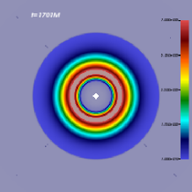
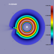
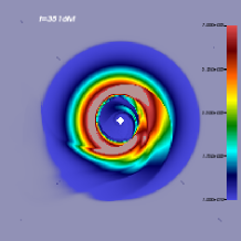
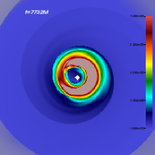
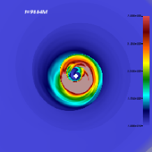
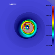
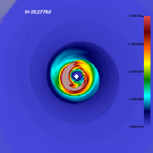
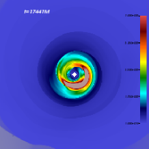
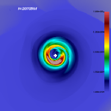
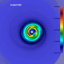
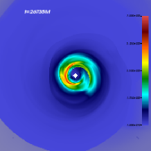
Figure 1: The rest-mass density of the perturbed torus during the time evolution for Model $P_{1}$, given in a linear color scale. The torus is perturbed by a matter coming from the outer boundary. The matter interacts with the torus around $t=3034M$ and distorts it. The local Papaloizou-Pringle instability is formed around $t=4540M$ and it is suppressed during the evolution. The structure of the torus is highly turbulent and makes quasi-periodic oscillation. The domain is $[X_{min},Y_{min}]\rightarrow[X_{max},Y_{max})]=[-120M,-120M)]\rightarrow[120M,120M]$.

In order to reveal the effect of the size of torus and inner radius onto the instability and dynamics of the torus, we consider the perturbations of the tori for the same mass, but with different sizes. The time evolution of the central rest-mass density of torus, each of them plotted along $r$ at $\phi=0$, are shown for models $P_{1}$ and $P_{3}$ in Fig.2 . For these models, we have applied a perturbation, which is $\rho_{p}=0.9\rho_{c}$, from the outer boundary between $t=0M$ and $t=80M$ to evolute the influence of perturbation to the overall dynamics of torus. The perturbation destroys the torus, triggers the Papaloizou-Pringle instability and can cause the location which has the maximum density to approach the horizon. Such perturbation induces the matter to fall into the black hole or out from computational domain. While the maximum rest-mass density of torus slightly oscillates for model $P_{1}$, seen in the right panel of Fig.2, the rest-mass density for model $P_{3}$ significantly decreases, seen in the left panel of the same graph, during the time evolution.

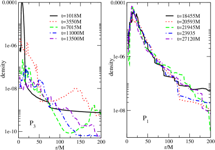
Figure 2: Time evolution of the rest-mass density along the r for model $P_{3}$ (left panel) and model $P_{1}$ (right panel). The portion of the density around the cusp location is also given for model $P_{1}$.

Accretion rate shows time variation in a great amplitude similar to one happening in low or hard X-ray time variation. Computing the accreting and the mass accretion rate are important indicators to understand the disc behavior and its instability around the black holes. The non-axisymmetric perturbation onto the steady-state torus, which has a constant specific angular momentum, around the black hole can describe the Papaloizou-Pringle instability. Instability of the accreted torus can be subject to perturbation coming from the outer boundary in a number of circumstances which may cause unstable mass accretion rates (Papaloizou & Pringle, 1984, 1985). We have confirmed that the accretion rate is governed by some physical parameters: the torus-to-hole mass ratio, the location of cusp, initial specific angular momentum of the torus, Mach number of the perturbed matter and the angular momentum of the black hole. The mass accretion rate computed from $P_{1}$, $P_{3}$, and $P_{4}$ are depicted in the left part of Fig.3. We have noticed that the mass accretion rate for the models are the same at early times of simulations, but later the mass accretion rate for models, $P_{3}$ and $P_{4}$, drop exponentially as a function of time and the Papaloizou-Pringle instability is developed. Interestingly, the mass accretion rate for only model $P_{1}$ does not increase in amplitude, and it oscillates around $dM/dt=5$ x $10^{-5}$.

The mass accretion rate of the perturbed torus produces luminosity associated with the central engine of gamma ray burst. The expected maximum accretion rate from the gamma ray burst is as high as $dM/dt\approx 0.01-1M_{\odot}/s$ (Chen & Beloborodov, 2007). Fig.3 indicates that the computed mass accretion rate from our numerical simulations, $\frac{dM}{dt}\sim$ 2 x $10^{5}(\frac{M_{\odot}}{s})\frac{dM}{dt}(geo)$ where $\frac{dM}{dt}(geo)$ is the mass accretion rate in geometrized unit, is in order of or slightly higher than the expected maximum accretion rate. It is also shown in the left panel of Fig.3 that the mass accretion rate suddenly increases after perturbation reaches to the torus and shortly after the Papaloizou-Pringle instability is developed. All the models in Fig.3 exhibit the Papaloizou-Pringle instability which grows exponentially with time and present a non-linear growth rate. After long time later (it is approximately $t=15000M$ for models $P_{5}$ and $P_{7}$), it reaches a saturation point and finally reaches a new quasi-equilibrium point. Before the saturation point, the torus looses mass and then it relaxes to the quasi-stationary accretion state.

It is obvious from the right part of Fig.3 that the accretion rates exponentially decay during the time and is always bigger when the mass ratio of the torus-to-black hole is larger. Decaying a mass accretion rate reaches a constant value $dM/dt\approx 0.1M_{\odot}/s$ around $t=14000M(t=82t_{orb})$. It is in good agreement with the expected accretion rates for accreting disc with the GRBs. As it can be seen in Fig.3, the amplitude of mass accretion rate and its behavior manifest a dependence on the mass ratio of the torus-to-black hole. While the mass accretion rates for all models decay with time due to the strong gravity which overcomes angular momentum of the torus, it oscillates around a certain rate for model $P_{1}$, shown in Fig.3. The oscillation behaviors of all models are seen during the time evolution. When the accreted torus gets close to the black hole and cusp moves outwards into the torus, model $P_{1}$ reaches persistent phase of quasi-periodic oscillation without the appearance of the Papaloizou-Pringle instability.

The continuous perturbation of the black hole-torus system can lead not only instability of the torus but also oscillates of its dynamics around the certain points, seen in Fig.4. The left panel in Fig.4 exhibits the time variation of mass accretion rate for model $P_{4}$ computed for $r=8M$ which is true for the perturbed matter injecting from the outer boundary continuously. The density of the torus at a fixed time $t=17200M$ and $\phi=0$ along $r$ is shown in the right panel. It is seen in this plot that the perturbation starts to interact with a torus around $t\sim 3000M$, and then nonlinear oscillation is developed. It is noted that the continuous perturbation can create different types of dynamical structures, accretion rates and shock wave on the disk.

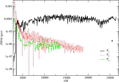
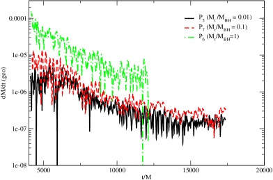
Figure 3: Left panel: the mass accretion rates for models $P_{1}$, $P_{3}$, and $P_{4}$ computed at $r=6M$ in geometrized unit. Three different models, the torus with different $r_{in}-r_{c}$ while keeping the same sound velocity or vice verse, are considered to show the effect of perturbation on the torus. Right panel: mass accretion rate for models $P_{5}$, $P_{6}$, and $P_{7}$.

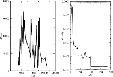
Figure 4: The mass accretion rate (left panel) and the rest-mass density of torus along r (right panel) are plotted for model $P_{2}$ .

Accretion into the black hole or out from the computational domain is driven by a transport of angular momentum via spiral shock waves created on the torus. The higher specific angular momentum of the torus outwards can allow the torus to become more stable. Fig.5 shows the specific angular momentum of the torus along the radial coordinate for models $P_{1}$, $P_{5}$, $P_{6}$, and $P_{7}$. The Keplerian specific angular momentum is also plotted at the top of these models to compare them. The specific angular momentum changes drastically depending on the radius. It becomes apparent that the increasing of the specific angular momentum outwards leads to stabilize the torus and suppresses the Papaloizou-Pringle instability, seen in Fig.1. The Papaloizou-Pringle instability visible immediately after the perturbation starts to influence of the stable torus. The Papaloizou-Pringle instability performs a torque on the torus and the angular momentum of the torus is redistributed. So it amplifies the mass accretion rate (Zurek & Benz, 1986). The rotating quasi-steady-state torus can only be seen in model $P_{1}$. Because the substantial amount of the specific angular momentum is kept inside the region $r<50M$. Meanwhile, it is seen in Fig.5 that specific angular momentum is sub-Keplerian which indicates that the gas pressure creates a pressure force and it supplies a radial support to the torus.

The newly developed angular momentum distribution of the black hole-torus system, after the non-axisymmetric perturbation, might have the local Rayleigh stability condition depending on the slopes and its signs. As you can see in Fig.5, the slope of the specific angular momentum is bigger than zero ($d\ell/dr>0$), which is the limit of the Rayleigh-stable torus, in model $P_{1}$ for $r<50M$, but it is $d\ell/dr<0$ and produces the Rayleigh-unstable torus for $50M<r<75M$. Any increase of the specific angular momentum in the radial direction stabilizes the torus.

Figure 5: The specific angular momentum for models $P_{1}$, $P_{5}$, $P_{6}$, and $P_{7}$ and for Keplerian are plotted as a function of radial coordinate a long time later that the disc is perturbed and instability is developed.

Fig.6 represents the time evolution of the maximum rest-mass density at the center of the torus, each of them normalized to their initial values, for models $P_{5}$, $P_{6}$, $P_{7}$, $P_{8}$, and $P_{9}$. For these models, we have applied the same perturbation with different densities ($\rho_{p}=0.9\rho_{c}$), giving the first kick to the black hole-torus system. The matter begins to influence the torus around $t=3120M$. The perturbation triggers the non-stable oscillation of the torus for models given in Fig.6 except the model $P_{8}$. These models exponentially decay and produce sharp peaks after perturbation reaches the torus. Thus, these results imply that subsonic or mildly supersonic perturbation produces the pressure-supported oscillating torus around the black hole, and amplitude of the oscillation gradually decreases while the Mach number of perturbation increases. Such oscillations can cause the matter to fall into the black hole or outward from the computational domain. These physical phenomena can significantly reduce the rest-mass density of the torus during the time evolution seen in Fig.6. Depending on the initial configurations, such as, mass ratio of the torus-to-hole and inner radius of the last stable orbit of the torus, the reducing rate of the rest-mass density is defined at the end of simulation. The density of the stable initial torus having an initial radius $r_{in}=5.49M$ given in model $P_{5}$ decreases slower than the one with the smaller inner radius given in models $P_{6}$, $P_{7}$, $P_{8}$, and $P_{9}$. This result is also confirmed by model $P_{1}$. The matter of the torus close to the black hole would fall into the black hole due to the strong gravity after the torus is triggered by perturbation. Therefore, the mass of the black hole and its spin would increase with time significantly. We also note that the reduction of the rest-mass density for model $P_{6}$ is slightly slower than the model $P_{7}$. So the lower the torus-to-hole mass ratio looses the faster the matter during the evolution. But it needs a further consideration to reveal a global conclusion.

Figure 6: The variation of the maximum density of torus in logarithmic scale as a function of time, each of them normalized to its initial value $\rho_{o}\equiv\rho_{c}$, for the models, $P_{5}$, $P_{6}$, $P_{7}$, $P_{8}$, and $P_{9}$. The torus loses the matter during the time evolution for all cases while it is almost stable before the perturbed matter reaches the torus.

3.2 Perturbed Torus Around the Rotating Black Hole

In order to put forth the effect of the rotating black hole onto the perturbed torus, we have perturbed the stable torus orbiting around the rotating black hole using the initial parameters given in models, $P_{10}$, $P_{11}$, and $P_{12}$ in Table 1. We have analyzed the time evolution of the rest-mass density of the torus with/without perturbation and found that perturbed torus given in model $P_{12}$ become unstable before the perturbation reaches to it but it is stable for model $P_{11}$. The period of fluid at the location of the highest density for model $P_{11}$ is $T_{c}=39.4M$. The structure of unperturbed torus on a fixed space-time metric background, called a Cowling approximation, never changes during the evolution shown in Fig.7. The top row of Fig.7 clearly shows that the torus in the Cowling simulation does not develop a Papaloizou-Pringle instability where steady state structure of torus remains almost constant during the evolution (i.e. at least $t\sim 11t_{orb}$). Because the negligible mass accretion rates through the cusp freeze the growth of the Papaloizou-Pringle instability modes in Cowling approximation (Hawley, 1991).

The perturbations on the torus having different inner radii and total mass produce diverse dynamics. As it can be seen in Fig.8 that the spiral pattern is produced around the rotating black hole, and it causes the gas falling into the black hole during the simulations. At the same time, it also creates regular oscillation seen in the second and third rows of Fig.7 and model $P_{11}$ in Fig.8. It is seen from the model $P_{12}$ in Fig.8 and, last two rows of Fig.7 that the torus responds somewhat differently to the applied perturbation, and the torus with a low mass, which is far away from the black hole, has a non-oscillatory behavior. Both of these models indicate that at the end of the simulation, the rest-mass density of the torus is reduced substantially. On the other hand, it is shown that the torus, which does not have a cusp point, is unstable even before the perturbation, and has a non-linear dynamic during the evolution as seen in the last two rows of Fig.7.

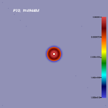
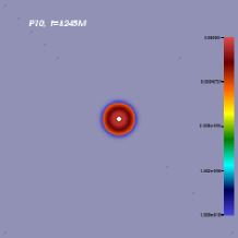
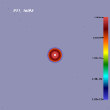
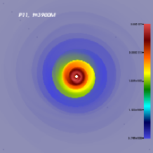
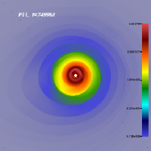
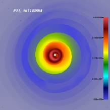
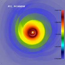
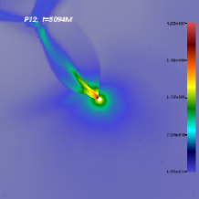
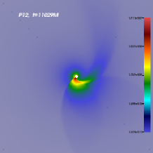
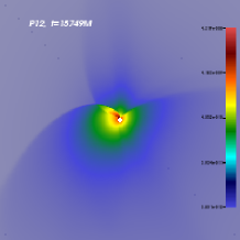
Figure 7: Density $\rho$ of the torus at the equatorial plane for different models, $P_{10}$, $P_{11}$, and $P_{12}$ with a black hole rotation parameter, $a=0.9$, given in a linear color scale. While the top row shows the unperturbed torus around the rotating black hole, the others indicate the perturbation of torus having different size and density. The domain is $[X_{min},Y_{min}]\rightarrow[X_{max},Y_{max})]=[-100M,-100M)]\rightarrow[100M,100M]$.

Figure 8: The time evolution of the rest-mass density at a fixed point on the torus for models, $P_{11}$ and $P_{12}$, for $a=0.9$. The inner radii of the models are different, but the same perturbation is applied to the both models.

3.3 Low-Density Perturbation

The dynamical respond of the black hole-torus system to perturbations presents incredible evidences about how the high-energetic phenomena occur close to the compact objects. In order to extract the information from these phenomena and to compare them with the observation, we need to understand the dynamics of the torus-black hole system in detail. In the previous subsections we have discussed the dynamical respond of this system to the high-density perturbation (i.e. $\rho_{p}=0.9\rho_{c}$). In addition to high-density perturbation we also perform a perturbative analysis with a low density (i.e. $\rho_{p}=10^{-4}\rho_{c}$), which is more realistic in the astrophysical system, to black hole-torus system. The all numerical results from high-density perturbation, low-density perturbation and non-perturbation are plotted and given in Figs. 9 and 10 for models $P_{3}$ and $P_{1}$, respectively.

The initial torus given in model $P_{3}$ in Table 1 is stable and its size is $r_{out}-r_{in}=11.319M$. The evolution of the rest-mass density of this torus without a perturbation is not exactly constant and slightly decay during the evolution due to the small amount of matter accreted onto the black hole (c.f. Fig.9). The similar trend was also found by Zanotti et.al. (2003). On the other hand, the instability is triggered by perturbation and the interaction of the size of the torus with a low- or high-density perturbation produces Papaloizou-Pringle instability, but the time of the formation of the instability for low-density perturbation is slightly larger than the high-density one. It is apparent from Fig.9 that the instability is fully developed and the highest rest-mass density of the torus reaches $\sim 50\%$ of its initial value in case of the low-density perturbation during the less than one orbital period ($t\sim 120M$ which equals to $\sim 0.79$ orbital period) just after the interaction, but it is $\sim 6\%$ in case of the high-density perturbation. A considerable amount of matter falls onto the black hole after the instability is developed and it oscillates during the time. And, the high-density perturbation causes the faster loss of matter if we compare with the low density perturbation. It is also noted that the oscillation properties of the black hole-torus system for both cases prominently different and they exponentially decrease over time. But the high-density perturbation case goes rapidly toward to zero. The development of the non-axisymmetric modes and comparison of the different physical parameters in the instabilities are explained in the next Subsection 3.4 in detail.

Revealing the impacts of the size of the torus, location of the inner radius of the torus and the severity of the density of the substance used as a perturbation is important to understand the physical mechanism in the astrophysical phenomena. Fig.10 represents how the different values of the rest-mass densities of perturbations affect the bigger size of the torus with a inner radius located at $r_{min}=15M$. The initial torus given in Fig.10 has size $57.99M$, which is almost $\sim 5$ times larger than the model $P_{3}$ and it is perturbed by low- and high-rest-mass density. It is observed that if the density of the perturbation is larger, accretion toward to the torus has a considerable amount and therefore a high amplitude quasi-periodic oscillation is developed very rapidly. On the other hand, if the magnitude of the rest-mass density of the perturbation is small, less mass accreates during the evolution. Hence more time will be needed to produce the instability and the quasi-periodic oscillation as shown in Fig10. In this case, oscillation grows slowly for a smaller accretion rate. In addition to these, it is also noted that the normalized rest-mass density in the case of the non-perturbation is almost constant.

We conclude this subsection by comparing Figs.9 and 10 that the size of torus, the location of the inner radius of the torus and the amount of the perturbation play an important role to determine the time of the formation of the Papaloizou-Pringle instability and the quasi-periodic oscillation in the black hole-torus system.

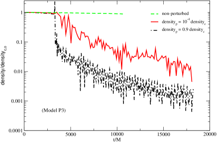
Figure 9: The evolution of the rest-mass density of the torus at the point, where the rest-mass density is maximum, for model $P_{3}$ with no-perturbation and with different values of densities of the perturbation in logarithmic scale. It is normalized to its initial value using the density at the computed point.

Figure 10: Same as Fig.9 but it is for model $P_{1}$ and linear scale is used.

3.4 Fourier Mode Analysis of the Instability of the Torus

The non-axisymmetric instabilities can be identified and characterized by using the linear perturbative studies of the black hole-torus system. The characterization of the instability, which is carried out by defining the azimuthal wave number $m$ and computing the saturation point, is performed from the simulation data by computing Fourier power in density. The Fourier modes $m=1$ and $m=2$ and growth rate are obtained at the equatorial plane (i.e. $\theta=\pi/2$) using the following equations given in De Villiers & Hawley (2002),

$$Im(w_{m}(r))=\int_{0}^{2\pi}\rho(r,\phi)sin(m\phi)d\phi,$$ (3)

$$Re(w_{m}(r))=\int_{0}^{2\pi}\rho(r,\phi)cos(m\phi)d\phi,$$ (4)

From the Eqs.3 and 4, the mode power is defined as

$$P_{m}=\frac{1}{r_{out}-r_{in}}\int_{r_{in}}^{r_{out}}ln\left([Re(w_{m}(r))]^{2}+[Im(w_{m}(r))]^{2}\right)dr,$$ (5)

where $r_{in}$ and $r_{out}$ are the inner and outer radii of the initially formed stable torus. The values of these radii are given in Table 1 for all models.

The growth of the main Papaloizou-Pringle instability modes in case of high- and low-density perturbations, and without any perturbation for model $P_{3}$ is given in Fig.11. The mode powers of $m=1$ and $m=2$ are shown as a function of time. It is shown that the modes grow significantly for torus. As expected, non-perturbed black hole-torus system does not present any mode growing during the evolution. After about $t=502M$ times which is equal to $t=3.3t_{orb}$ orbital period, the torus starts to develop $m=1$ and $m=2$ non-axisymmetric modes and these modes undergo exponential growth until $t=757M$ strongly. Both modes grow together until about $t=1741M$. They diverge at this time and converge again at the saturation point. The saturation point represents the largest value of the mode amplitude which is reached at $t_{sat}=3351M$ (i.e. $t_{sat}=22t_{orb}$) for modes $m=1$ and $m=2$. It is important to note that the non-axisymmetric dynamics survives with an remarkable amplitude even after the saturation of the Papaloizou-Pringle instability. Meanwhile, the $m=2$ mode shows more erratic behavior between $t=1741M$ and $t=3351M$. The $m=1$ deformation for the low-density perturbation, $\rho_{p}=10^{-4}\rho_{c}$, is slightly different than the high-density perturbation. The exponential growth in the high-density perturbation stars at later time (i.e. $t=990M$) and reaches its peak value at $t=4542M$ which is called the saturation point.

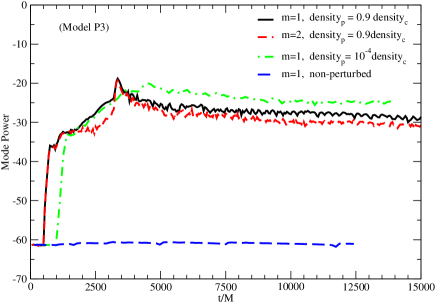
Figure 11: Evolution of the modes growth for perturbed and non-perturbed torus around the black hole for an initial data given in model $P_{3}$.

Unlike the model $P_{3}$, the amplitudes at the saturation points of $m=1$ and $m=2$ modes do not coincide for model $P_{1}$. The maximum amplitude of the $m=1$ mode is always larger, but the saturation times for both modes almost equal to each other, $t_{sat}=5681M$ ($t_{sat}=7.2t_{orb}$) for $\rho_{p}=0.9\rho_{c}$ and $t_{sat}=13889M$ ($t_{sat}=17.7t_{orb}$) for $\rho_{p}=10^{-4}\rho_{c}$ as shown in Fig.12. The $m=1$ and $m=2$ modes grow rapidly regardless of the initial values of the perturbations. But the mode in the high-density perturbation starts to grow early than the low-density one. After they reach to the saturation point, the behaviors of the mode powers almost remain the same during the rest of the simulation (c.f. the inset of Fig.12.) The difference between the saturation points of the high- and low-density perturbations is $t=8232M$ $(t=10.5t_{orb})$.

The mode power given in Figs.11 and 12 and the mass accretion rate given in the left panel of the Fig.3 clearly show that the significant mass accretion appears when the growing mode of the Papaloizou-Pringle instability reaches to the saturation point. It happens due to the spiral wave generated as a consequence of interaction between black hole-torus system and matter used as a perturbation. The spiral wave, and therefore, Papaloizou-Pringle instability transports the angular momentum of the torus through the co-rotation radius.

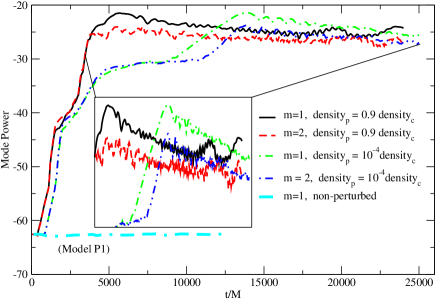
Figure 12: Same as Fig.11 but for model $P_{1}$.

Mode powers of $m=1$ deformations for non-rotating black hole with a small (model $P_{3}$) and bigger (model $P_{1}$) sizes of an initial tori, and for a rotating black hole (model $P_{11}$) are computed and given in Fig.13. As it is displayed in Fig.13, the growing times, maximum amplitude and developed saturation points of the m=1 non-axisymmetric mode are modified by the size of the torus, the black hole spin and the density of the perturbation. The interaction of the non-axisymmetric $m=1$ deformation with a black hole spin leads to the formation of a high-amplitude in the growth rate and it reaches to the saturation point. While the maximum mode power of the Papaloizou-Pringle instability is weak for the bigger size of the torus, it has vigorous one for small size of torus and torus around the rotating black hole. It is hard to define the exact definition of the saturation time because of the weak-maximum power mode.

Figure 13: The m=1 growing mode amplitude for different models, $P_{1}$, $P_{3}$ and $P_{11}$. Models $P_{1}$, $P_{3}$ are for the different size of the torus around the non-rotating black hole but $P_{11}$ represents the $m=1$ mode for the perturbed torus around the rotating black hole.

3.5 QPOs from the oscillating Torus

We have performed the simulations using different values of $\ell_{0}$, $r_{cusp}$, $r_{in}$ and $r_{c}$ of the initial torus with a perturbation given in Table 1. For these initial perturbed discs, the global oscillations are seen at various frequencies. The frequencies of oscillating torus are computed by using the proper time. The unit of the computed frequency is in the geometrized unit and it is translated to Hertz of frequency using the following equation,

$$f(Hz)=f(M)\times 2.03027\times 10^{5}\times\left(\frac{M_{\odot}}{M}\right),$$ (6)

where $M$ is the mass of black hole, $f(M)$ is the frequency in the geometrized unit, $M_{\odot}$ is the solar mass and $f(Hz)$ is the frequency in $Hz$. Applying a perturbation to a perfectly stable torus gives rise to an epicyclic motion in radial direction due to the oscillation mode. The radial epicyclic frequency is the frequency of the displaced matter oscillating in radial direction. Fig.14 consists of a fundamental frequency at $\sim 199Hz$ and number of overtones, which are the results of the non-linear couplings, $\sim 399Hz$, $\sim 600Hz$ , $\sim 800Hz$ etc. that they can determine the ratios 1:2:3:…. It suggests that the non-linear oscillation of the torus due to the perturbation is a consequence of fundamental modes of the torus. The power law distribution given in the right panel of Fig. 14 indicates how the peaks appear as a function of $\phi$ at fixed $r=8.12M$ which almost represents the point of maximum density of the torus. The amplitudes for the corresponding peaks are almost the same for all $\phi$ at the same frequencies. In both graphs, two strong narrow peaks locate at $\sim 199Hz$ and $\sim 399Hz$. Fig. 14 also indicates that QPO frequencies are global and just confined within the torus. We note from a long history of experience in our numerical models that the computed QPO frequencies do not depend on the excision radius defined in Boyer-Lindquist coordinate. The QPO behavior of the oscillating torus found in our work might be used to explain commensurability frequencies observed in the sources, $H1743−322$, $XTE$ $J1550–564$, and $GRS$ $1915+105$ (McClintock & Remillard, 2004).

The QPO’s frequencies from our simulation for the black hole $M=2.5\,M_{\odot}$ are approximately the same as found in Zanotti & Rezzolla (2003); Zanotti et.al. (2003). They computed the power spectrum of the $L_{2}$ norm error of the rest-mass density for different $\eta$ after the long time evolution. The fundamental frequencies, which are seen around $200Hz$, and the series of overtones for both cases are observed. Our study indicates that the perturbed torus, which is caused either by the introduction of a suitable parametrized perturbation to the radial velocity done by Zanotti & Rezzolla (2003); Zanotti et.al. (2003) or by a matter coming from the outer boundary toward the torus (our simulations), produces regular oscillatory behavior. The modes observed from both perturbations are called the pressure $(p)$ mode of oscillation of the torus. The small size of accretion torus orbiting around the black hole can be used to explain $p$ mode in high frequency quasi-periodic oscillations (Rezzolla et.al., 2003). The $p$ mode represents the oscillation of matter in the horizontal direction at the equatorial plane and is trapped inside the torus. As shown in Figs.1 and 3, the structure of the torus changes significantly due to the angular momentum transport of the torus. So the $p$ mode is able to survive during the evolution. Due to the two-dimensional structure of the system, the magnetic field did not create a strong effect on the wave properties of $p$ mode(Fu & Lai, 2011).

It is known from previous discussion that the torus loses matter during time evolution, and it has chaotic behavior seen in models $P_{3}$ and $P_{4}$. Due to this irregular non-linear oscillation, only a fundamental mode appears, but their overtones are absent in the power spectrum when the torus is initially more close to the black hole. We suggest that the variation of the torus’s matter results from the non-spherically symmetric perturbation of the inner accreted torus.

We have also analyzed the time evolution of mass accretion rate for the model, $P_{11}$ reported in Table 1 to compute Fourier spectra of the perturbed torus around the rotating black hole. After the perturbation starts to influence the torus dynamics, mass accretion rate oscillates around its quasi-equilibrium point. Due to a distinctive quasi-periodic oscillation of the unstable torus, the periodic character of the spiral structure becomes more evident after perturbation reaches to the torus a long time later. After the torus relaxes to regular oscillation, it loses the mass, and the oscillation amplitude decreases during the evolution. The computing QPO frequencies from the mass accretion rate might not give definite information, but we may approximately predict it. The power spectra of mass accretion rate shows a fundamental mode with a strong amplitude at $500Hz$ and series of overtones, as a consequence of the non-linear couplings, located at $1001Hz$, $1491Hz$, and $1998Hz$ for $a=0.9$ and $M=2.5\,M_{\odot}$. It is worth emphasizing that a fundamental frequency from the torus around the rotating black hole is much larger than the non-rotating case seen in Table 2. This is an acceptable result because the torus is more closer, and gravity is more stronger in case of the rotating black hole. Table 2 also suggests that a linear scaling is presented for the black hole spin.

The observed high frequency QPOs around the black holes and neutron stars were described by Kluzniak & Abramowicz (2001); Abramowicz & Kluzniak (2001); Blaes et.al. (2007); Mukhopadhyay (2009); Mukhopadhyay et.al. (2012) using a single model which has addressed the variation of QPO frequencies. Based on the proposed model, they had predicted the spin of the black hole using the observed QPO pairs which seem to appear at a $3:2$ ratio. The lower and higher frequencies of pairs for any system are $\nu_{l}=\nu_{\perp}-\nu_{s}/2$ and $\nu_{h}=\nu_{r}+\nu_{s}$, respectively. Here, $\nu_{\perp}$, $\nu_{r}$ and $\nu_{s}$ are theoretical values of radial, vertical epicyclic frequencies (Dönmez, 2007) and spin frequency of the black hole, respectively. Using the above model we find that the computed commensurable frequency, $600:399$, is exposed at $\sim 8.1M$. The estimated value of location of resonance from numerical computation, which is $\sim 9M$, is in the suitable range of theoretical calculation.

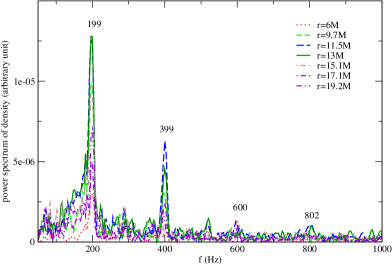
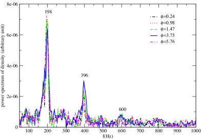
Figure 14: Power spectrum of the rest-mass density at a single point (any $\phi$ or $r$) for $M=2.5\,M_{\odot}$ for model $P_{1}$ shown in Table 1. A fundamental frequency appears at far left of the both graphs. The others are the consequence of overtones. The computed frequencies at any $r$ or $\phi$ overlap.

Table 2: The frequencies of genuine mode and its series of overtones, due to the nonlinear coupling, inside the torus from the evolution of mass accretion rate. It is computed for different black hole spins while the mass of the black hole is assumed to be $M=2.5\,M_{\odot}$.

Model	$a/M$	$f_{1}[Hz]$	$o_{1}[Hz]$	$o_{2}[Hz]$	$o_{3}[Hz]$
$P_{1}$	$0.0$	$199$	$399$	$600$	$800$
$P_{11}$	$0.9$	$500$	$1001$	$1491$	$1998$

4 Conclusion

We have performed the numerical simulation of the perturbed accreted torus around the black hole and uncovered the oscillation properties to compute QPOs. Instead of giving a perturbation to the radial velocity or to the density of the stable torus studied by different authors in literature, the matter is sent from the outer boundary toward the torus-black hole system to perturb it. We have initially considered the different sizes of the stable tori and torus-to-hole mass ratios to expose oscillations of the tori, and computed the fundamental modes and their overtones which results from the excitation of frequencies due to perturbation.

We have confirmed that the torus around the black hole might have a quasi-periodic oscillation only if we choose a suitable initial data for a stable accretion torus. There are a number of different physical parameters which may affect the oscillation properties of the torus. It is seen from our numerical simulations that the size of torus and its initial radius affect the frequencies of oscillating torus and their overtones. The size of torus and its rest-mass density also influence the time of onset of the instability and the power of oscillations and, this oscillation creates radiation of hotter photons. The similar conclusion has been also confirmed by Bursa (2005). The oscillation and mass losing rate of the perturbed torus strongly depend on the Mach number of perturbing matter. Upon the given appropriate parameters of perturbation, the subsonic or mildly supersonic flow produces the pressure-supported oscillating torus around the black hole and the amplitude of oscillation gradually decreases while the Mach number of perturbation increases. For the most of the models given in Table 1, we have found that the rest-mass density of the torus substantially decreases due to the Papaloizou-Pringle instability which is developed as a consequence of interaction between the propagation of waves across the co-rotation radius. The mode powers of $m=1$ and $m=2$ grow as a function of time. It is depicted that the modes grow significantly for torus. On the other hand, a torus which has a bigger inner radius and size, develops a new inner radius and cusp location after a perturbation. During this progress, a Papaloizou-Pringle instability is developed. Later, the black hole-torus system reaches a new quasi-steady state and does not present a Papaloizou-Pringle instability. Thus, the inner radius, the specific angular momentum of torus, size of the torus, and Mach number and density of the perturbation play a critical role in the onset of the Papaloizou-Pringle instability.

Our studies also indicate that QPOs are common phenomena on the disc around the black holes. If the accretion disc or torus have a quasi-periodic behavior, it emits continuous radiation during the computation. The amplitude of oscillation is excited by nonlinear physical phenomena. It has been explained in terms of the excitation of pressure gradients on the torus and it is called $p$ mode. It is shown that the power law distribution of oscillating stable torus includes a fundamental frequency at $\sim 199Hz$ and their number of overtones, $\sim 399Hz$, $\sim 600Hz$, and $\sim 800Hz$ that they can determine the ratios $1:2:3:4$. These frequencies are observed at any radial and angular directions of the torus. The computed QPO frequencies are almost the same as the ones given by Zanotti & Rezzolla (2003); Zanotti et.al. (2003) even though they apply a perturbation to the radial velocity or to the density of the stable torus in order to have an oscillation. The mode called as p is also the same in both simulations. We have also confirmed that the fundamental QPO frequencies and their overtones for a rotating black hole are much higher than the non-rotating case due to strong gravity and location of the inner radius of the accreted torus. The strong gravity plays a dominant role in the high frequency modulation of observed X-ray flux in the binary system (Bursa et.al., 2004). It is consistent with the computation from our simulations seen in Table 2.

Finally, we have performed the numerical simulation using $2D$ code on the equatorial plane. Clearly, to investigate the effects of forces in the vertical direction on the torus instability that may play an important role on the dynamics of the whole system, $3D$ numerical simulations are required. The mode coupling in the vertical direction is likely to affect the instability of a perturbed torus-black hole system. Therefore, we plan to model the same perturbed system by using $3D$ code in the future.

References

- Abramowicz & Fragile (2013) Abramowicz, M. A. & Fragile, P. C. 2013, Living Rev. Relativity, 16, arXiv:1104.5499.
- Abramowicz et.al. (1983) Abramowicz, M. A., Calvani, M. & Nobili, L. 1983, Nature, 302, 597-599.
- Abramowicz & Kluzniak (2001) Abramowicz, M. A., & Kluzniak, W. 2001, A&A, 374, L19-L20.
- Abramowicz et.al. (1978) Abramowicz, M. A., Jaroszynski, M. & Sikora, M. 1978, A&A, 63, 221-224.
- Blaes et.al. (2007) Blaes, O. M., Sramkova, E., Abramowicz, M. A., Kluzniak, W. & Torkelsson, U. 2007, ApJ, 665, 642-653.
- Blaes & Glatzel (1986) Blaes, O. M. & Glatzel W. 1986, MNRAS, 220, 253.
- Burkert et.al. (2012) Burkert, A., Schartmann, M., Alig, C., Gillessen, S., Genzel, R., Fritz, T. K. & Eisenhauer, F. 2012, ApJ, 750, 58B.
- Bursa (2005) Bursa, M. 2005, Astron.Nachr. 326, 849-855.
- Bursa et.al. (2004) Bursa, M., Abramowicz, M. A., Karas, V. & Kluzniak, W. 2004, ApJ, 617, L45-L48.
- Chen & Beloborodov (2007) Chen, W. & Beloborodov, A. M. 2007, ApJ, 657, 383.
- Coward et.al. (2002) Coward, D. M., van Putten, M. H. P. M., & Burman, R., R. 2002, ApJ, 580, 1024.
- Daigne & Font (2004) Daigne, F. & Font, J. A. 2004, MNRAS, 349, 841.
- De Villiers & Hawley (2002) De Villiers, J.-P. & Hawley, J. 2002, ApJ, 577, 866.
- Dönmez et.al. (2011) Dönmez O., Zanotti, O., & Rezzolla, L. 2011, MNRAS, 412, 1659.
- Dönmez (2004) Dönmez O. 2004, Astrophys. Spac. Sci., 293, 323.
- Dönmez (2007) Donmez O. 2007, MPLA, 22, 141-157.
- Font & Daigne (2002) Font, J. A. & Daigne, F. 2002, MNRAS, 334, 383.
- Font et.al. (2000) Font, J.A., Miller, M., Suen, W.-M. & Tobias, M. 2000, Phys. Rev. D, 61, 044011.
- Fu & Lai (2009) Fu, W. & Lai, D. 2009, ApJ, 690, 1386.
- Hawley (1991) Hawley J. F. 1991, ApJ, 381, 496.
- Kluzniak & Abramowicz (2001) Kluzniak, W. & Abramowicz, M. A. 2001, astro-ph/0105057.
- Korobkin et.al. (2013) Korobkin, O., Abdikamalov, E., Stergioulas, N., Schnetter, E., Zink, B., Rosswog, S. & Ott, C. 2013, MNRAS, 431, 349-354.
- Kiuchi et.al. (2011) Kiuchi, K., Shibata, M., Montero, P. & Font, J., A. 2011, Physical Review Letters, 106, 251102
- Lee (2004) Lee, H., K. 2004, Journal of Korean Physical Society, 45, 1746.
- Levinson & Blandford (1996) Levinson, A. & Blandford, R. 1996, ApJ, 456L, 29L.
- McClintock & Remillard (2004) McClintock J. E. & Remillard R. 2004, in LewinW. H. G., van der Klis M., eds, Compact Stellar X-Ray Sources. Cambridge University Press, Cambridge.
- Meszaros (2006) Meszaros, P. 2006, Rep. Prog. Phys., 69, 2259.
- Montero et.al. (2010) Montero, P. J., Font, J. A. & Shibata, M. 2010, PRL, 104, 191101.
- Montero et.al. (2007) Montero, P. J., Zanotti, O., Font, J. A. & Rezzolla, L 2007, MNRAS, 378, 1101.
- Moscibrodzka et.al. (2006) Moscibrodzka, M., Das, T. K. and Czerny, B. 2006, MNRAS, 370, 219.
- Mukhopadhyay (2009) Mukhopadhyay, B. 2009, ApJ, 694, 387-395.
- Mukhopadhyay et.al. (2012) Mukhopadhyay, B., Bhattacharya, D. & Sreekumar, P. 2012, IJMPD, 21, 1250086.
- Nagar et.al. (2005) Nagar, A., Font, J. A., Zanotti, O. & de Pietri, R. 2005, PRD, 72, 024007.
- Papaloizou & Pringle (1984) Papaloizou, J. C. M. & Pringle, J. E. 1984, MNRAS, 208 721.
- Papaloizou & Pringle (1985) Papaloizou, J. C. M. & Pringle, J. E. 1985, MNRAS, 213 799.
- Rees & Meszaros (1994) Rees M. J. & Meszaros P. 1994, ApJL, 430, L93.
- Remillard et.al. (1999) Remillard, R. A., Morgan, E. H., McClintock, J. E., Bailyn, C. D. & Orosz, J. A. 1999, ApJ, 522, 397-412.
- Rezzolla et.al. (2003) Rezzolla L, Yoshida S and Zanotti O 2003a, MNRAS, 344, 978.
- Schnittman & Krolik (2008) Schnittman, J. D. & Krolik, J. H. 2008, 684, 835.
- Schnittman & Rezzolla (2006) Schnittman, J & Rezzolla, L. 2006, ApJ, 637L, 113S.
- Strohmayer (2001) Strohmayer, T. E. 2001, ApJ, 552, L49.
- van der Klis (2004) van der Klis M 2004, eprint arXiv:astro-ph/0410551.
- Fu & Lai (2011) Fu, W., & Lai, D. 2011, MNRAS, 410, 1617.
- Yildiran & Dönmez (2010) Yildiran, D. & Dönmez O. 2010, IJMPD, 19, 2111-2133.
- Zanotti et.al. (2003) Zanotti O, Rezzolla L and Font J A 2003, MNRAS, 341, 832.
- Zanotti et.al. (2005) Zanotti, O., Font, J. A., Rezzolla, L. & Montero, P. J. 2005, MNRAS, 356, 1371.
- Zanotti & Rezzolla (2003) Zanotti, O & Rezzolla, L. 2003 MSAIS, 1, 192.
- Zurek & Benz (1986) Zurek, W., H. & Benz, W. 1986, ApJ 308, 123.