Awaking the vacuum with spheroidal shells

Abstract

It has been shown that well-behaved spacetimes may induce the vacuum fluctuations of some nonminimally coupled free scalar fields to go through a phase of exponential growth. Here, we discuss this mechanism in the context of spheroidal thin shells emphasizing the consequences of deviations from spherical symmetry.

I Introduction

In a recent paper, it was shown that certain well-behaved spacetimes are able to induce an exponential enhancement of the vacuum fluctuations of some nonminimally coupled free scalar fields lv . This “vacuum awakening mechanism” may have consequences, in particular, to astrophysics, since the vacuum energy density of the scalar field can grow as large as the nuclear density of neutron stars in few milliseconds once the effect is triggered lmv . As a result, the system must evolve into a new equilibrium configuration and eventually it should induce a burst of free scalar particles llmv (see also Ref. novak98 -rdans12 for related classical analyses reaching similar conclusions). Conversely, the existence of classes of nonminimally coupled scalar fields can be unfavored by the determination of the mass-radius ratio of relativistic stars with known equations of state.

It is, thus, interesting to know if the main features described in Ref. lmv are preserved when assumptions as staticity and spherical symmetry are relaxed. In this paper, we investigate the vacuum awakening mechanism in the context of thin static spheroidal shells. This will allow us to explore the consequences of deviations from sphericity, while avoiding complications concerning uncertainties about the interior spacetime of nonspherical compact sources.

The paper is organized as follows. In Sec. II, we follow Ref. mccrea and present the general properties of the shell spacetime, emphasizing the assumptions which were made in order to obtain the particular class of solutions that we investigate. In Sec. III, we consider the quantization of a real scalar field in this background and proceed to discuss the vacuum awakening effect in nonspherical configurations. We show, in particular, that in the limit where spherical symmetry is recovered our results can be expressed in terms of known functions. In Sec. IV, we discuss the exponential growth of the vacuum energy density in the context of spherically-symmetric shells. Section V is dedicated to conclusions. We assume natural units in which $c=\hbar=G=1$ and metric signature $(-+++)$ throughout the paper.

II Thin spheroidal shells

Let us consider a static and axially-symmetric thin shell surrounded by vacuum thinshell1 -poisson . The most general line element describing the external- and internal-to-the-shell portions of the spacetime complying with the assumptions above can be written as synge

$$ds^{2}=-e^{2\lambda}dt^{2}+e^{2(\nu-\lambda)}(d\rho^{2}+dz^{2})+\rho^{2}e^{-2\lambda}d\varphi^{2},$$ (1)

where $\lambda=\lambda(\rho,z)$ and $\nu=\nu(\rho,z)$ satisfy

$$\frac{\partial^{2}\lambda}{\partial\rho^{2}}+\frac{\partial^{2}\lambda}{\partial z^{2}}+\frac{1}{\rho}\frac{\partial\lambda}{\partial\rho}=0,$$ (2)

$$\frac{\partial\nu}{\partial\rho}=\rho\left[\left(\frac{\partial\lambda}{\partial\rho}\right)^{2}-\left(\frac{\partial\lambda}{\partial z}\right)^{2}\right],$$ (3)

and

$$\frac{\partial\nu}{\partial z}=2\rho\frac{\partial\lambda}{\partial\rho}\frac{\partial\lambda}{\partial z}.$$ (4)

The external- and internal-to-the-shell regions will be covered with coordinates $(t,\rho,z,\varphi)$ and $(\bar{t},\bar{\rho},\bar{z},\bar{\varphi})$, respectively, where we will denote by $\cal{S}$ the 3-dimensional timelike boundary between them. It is worth to note that by using the spacetime symmetries one can choose the time and angular coordinates on $\cal{S}$ such that $\bar{t}=t$ and $\bar{\varphi}=\varphi$. As a result, we will denote the internal coordinates simply as $(t,\bar{\rho},\bar{z},\varphi)$ and the shell is identified with $t={\rm const}$ sections of $\cal{S}$. Let us assume, moreover, that the shell lies on a $\lambda={\rm const}$ surface:

$$\lambda(\rho,z)|_{\cal{S}}=\lambda(\bar{\rho},\bar{z})|_{\cal{S}}=\lambda_{0}=\textrm{const}.$$ (5)

This choice leads the spacetime inside the shell to be flat with the corresponding line element being cast as mccrea

$$ds^{2}_{-}=-e^{2\lambda_{0}}dt^{2}+e^{-2\lambda_{0}}(d\bar{\rho}^{2}+d\bar{z}^{2}+\bar{\rho}^{2}d\varphi^{2}).$$ (6)

In order to analyze the external metric, it is convenient to perform the coordinate transformation $\{\rho,z\}\to\{x,y\}$ defined by

$$\rho\equiv a(x^{2}-1)^{1/2}(1-y^{2})^{1/2},\;\;\;z\equiv axy,$$ (7)

where $x\in[1,\infty)$, $y\in[-1,1]$, and $a={\rm const}>0$. In terms of the $x$ and $y$ coordinates, Eq. (2) reads

$$\frac{\partial}{\partial x}\left[(x^{2}-1)\frac{\partial\lambda}{\partial x}\right]+\frac{\partial}{\partial y}\left[(1-y^{2})\frac{\partial\lambda}{\partial y}\right]=0.$$ (8)

The most general solution of Eq. (8) which is regular on $y=\pm 1$ (symmetry axis) and well behaved at $x\to\infty$ (spatial infinity) can be cast as

$$\lambda=\sum_{j=0}^{\infty}{A_{j}Q_{j}(x)P_{j}(y)},\;\;\;A_{j}={\rm const},$$ (9)

where $P_{j}(z)$ and $Q_{j}(z)$ are the zero-order associated Legendre functions of first and second kinds abramowitz , respectively. For the sake of simplicity, we will restrict ourselves to the particular class of spheroidal shells obtained by imposing $A_{j}=0$ for $j=1,2,\ldots$ in Eq. (9). As a result, we have

$$\lambda=-\frac{\beta}{2}\ln\frac{x+1}{x-1},$$ (10)

where $\beta=-A_{0}>0$ will play the role of a geometric parameter linked to the shell shape. It is worthwhile to note that condition (5) combined with the $A_{1}=A_{2}=\ldots=0$ choice restrict the possible shapes and stress-energy-momentum distributions of the shells considered here (see, e.g., Ref. quevedo for more general shells). Still, this class of shells is general enough for our purposes.

Equation (10) implies that the shells which we consider will lie on

$$x=x_{0}={\rm const}>1$$

surfaces. The corresponding $\nu$ solution can be directly obtained from Eqs. (3)-(4):

$$\nu=\frac{\beta^{2}}{2}\ln\frac{x^{2}-1}{x^{2}-y^{2}}.$$ (11)

By combining these results, the exterior metric will read

$$ds^{2}_{+} =-\left(\frac{x-1}{x+1}\right)^{\beta}dt^{2}+a^{2}\left(\frac{x+1}{x-1}\right)^{\beta}\left(\frac{x^{2}-1}{x^{2}-y^{2}}\right)^{\beta^{2}}$$

$$\times(x^{2}-y^{2})\left(\frac{dx^{2}}{x^{2}-1}+\frac{dy^{2}}{1-y^{2}}\right)$$

$$+a^{2}\left(\frac{x+1}{x-1}\right)^{\beta}(x^{2}-1)(1-y^{2})d\varphi^{2}.$$ (12)

One can see that the spacetime is asymptotically flat by taking the $x\to+\infty$ limit in Eq. (12). It will be shown later that $0<\beta<1$, $\beta=1$, and $\beta>1$ are associated with prolate, spherical, and oblate configurations, respectively.

Next, we must impose continuity of the internal and external induced metrics, $h_{ab}$, on $\cal{S}$. It is convenient to cover $\cal{S}$ with coordinates $\zeta^{a}=(t,y,\varphi)$, $a=0,2,3$, since the shell lies at $x=x_{0}={\rm const}$. The continuity condition establishes a relationship between the internal, $\bar{\rho},\bar{z},$ and external, $y$, coordinates on $\cal{S}$. For further convenience, however, let us replace coordinates $\bar{\rho},\bar{z}$ by $\tilde{r},\theta$ as defined below:

$$\bar{\rho}\equiv a\tilde{r}\sin\theta,\;\;\;\bar{z}\equiv a\tilde{r}\cos\theta.$$

By doing so, Eq. (6) reads

$$ds^{2}_{-} =-\left(\frac{x_{0}-1}{x_{0}+1}\right)^{\beta}dt^{2}+a^{2}\left(\frac{x_{0}+1}{x_{0}-1}\right)^{\beta}$$

$$\times\left(d\tilde{r}^{2}+\tilde{r}^{2}d\theta^{2}+\tilde{r}^{2}\sin^{2}\theta d\varphi^{2}\right),$$ (13)

where we have used $\lambda_{0}=-(\beta/2)\ln[(x_{0}+1)/(x_{0}-1)]$. Then, in order to join the metrics given by Eqs. (12) and (13) on $\cal{S}$, we impose $\tilde{r}|_{\cal S}=f(y)$ and $\cos\theta|_{\cal S}=g(y)$, where

$$f(y)=\left[\frac{(x_{0}^{2}-1)(1-y^{2})}{1-g(y)^{2}}\right]^{1/2}$$ (14)

and

$$\frac{g^{\prime}(y)(1-y^{2})}{1-g(y)^{2}} =g(y)y+(1-g(y)^{2})^{1/2}$$

$$\times\left[\left(\frac{x_{0}^{2}-1}{x_{0}^{2}-y^{2}}\right)^{\beta^{2}-1}-y^{2}\right]^{1/2}$$ (15)

with $``\;^{\prime}\;"\equiv d/dy$. The $f(y)$ function follows immediately after $g(y)$ is determined from Eq. (15) through a numerical calculation, where we fix $g(0)=0$ (to harmonize with the solution $g(y)=y$ for $\beta=1$). In order to guarantee that $g(y)$ is real, an extra restriction on $x_{0}$ must be imposed when $\beta>1$:

$$\beta>1 \Rightarrow x_{0}\geq\beta,$$ (16)

$$0<\beta\leq 1 \Rightarrow x_{0}>1.$$ (17)

For $\beta=1$, Eq. (17) just reflects the fact that the radius of a spherical shell must be larger than the Schwarzschild one.

In order to investigate the dependence of the shell shape on $\beta$ and $x_{0}$, we calculate

$$n \equiv L_{\textrm{equatorial}}/L_{\textrm{meridional}}$$

$$=\frac{(1-1/x_{0}^{2})^{(1-\beta^{2})/2}}{{}_{2}F_{1}(1/2,(\beta^{2}-1)/2,1;x_{0}^{-2})},$$ (18)

where $L_{\textrm{meridional}}$ and $L_{\textrm{equatorial}}$ are the meridional ($\varphi=\textrm{const}$) and equatorial ($y=0$) proper lengths, respectively, taken on some $t={\rm const}$ hypersurface and ${}_{2}F_{1}(a,b,c;z)$ is the hypergeometric function. We note that the shell will be prolate ($0<n<1$), spherical ($n=1$), and oblate ($n>1$) for $0<\beta<1$, $\beta=1$, and $\beta>1$, respectively (see Fig. 1). The maximum oblateness (associated with the maximum $n$ value) can be obtained from Eq. (18) combined with Eq. (16):

$$n_{\textrm{max}}\equiv\lim_{x_{0}=\beta\to\infty}{n}={e^{1/4}}/{I_{0}(1/4)}\approx 1.3,$$ (19)

where $I_{\nu}(z)$ is the modified Bessel function of first kind. This limit should not be viewed as a general restriction to arbitrary oblate shells but rather a consequence of the assumptions discussed below Eq. (10). There is no similar restriction for prolate configurations, since $n$ may take arbitrarily small (positive) values. For the sake of further convenience, it is also useful to calculate, at this point, the shell proper area as a function of $\beta$ and $x_{0}$:

$$A =4\pi x_{0}^{2}a^{2}\left(\frac{x_{0}+1}{x_{0}-1}\right)^{\beta}\left(1-\frac{1}{x_{0}^{2}}\right)^{(\beta^{2}+1)/2}$$

$$\times{}_{2}F_{1}\left(\frac{1}{2},\frac{\beta^{2}-1}{2},\frac{3}{2};\frac{1}{x_{0}^{2}}\right).$$ (20)

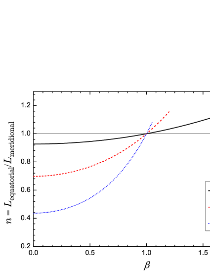
Figure 1: The ratio $n\equiv L_{\textrm{equatorial}}/L_{\textrm{meridional}}$ is plotted as a function of $\beta$ for shells lying at different values of $x_{0}={\rm const}$. For $0<\beta<1$, $\beta=1$, and $\beta>1$ we have prolate ($0<n<1$), spherical ($n=1$), and oblate ($n>1$) shells, respectively. The maximum value of $n$, $n_{\rm max}\approx 1.3$, corresponds to an oblate configuration lying at $x=x_{0}=\beta\to\infty$ for which the equatorial diameter is about twice as large as the polar one. Shells with $n\to 0$ correspond to infinitely thin and long rods, $0<\beta<1$, lying at $x=x_{0}\to 1$.

By establishing the interior and exterior metrics, the shell stress-energy-momentum tensor is also fixed:

$$T^{\mu\nu}=S^{ab}e^{\mu}_{a}e^{\nu}_{b}\delta(\ell),$$ (21)

where $\ell$ is the proper distance along geodesics intercepting orthogonally $\cal{S}$ (such that $\ell<0$, $\ell=0$, and $\ell>0$ inside, on, and outside $\cal{S}$, respectively), $e_{a}^{\mu}\equiv\partial x^{\mu}/\partial\zeta^{a}$ are the components of the coordinate vectors $\partial/\partial\zeta^{a}$ defined on $\cal{S}$ (with $\{x^{\mu}\}$ being some smooth coordinate system covering a neighborhood of $\cal{S}$ poisson ), and

$$S^{ab}=-\frac{1}{8\pi}(\Delta K^{ab}-h^{ab}\Delta K).$$ (22)

Here, $K_{ab}$ is the extrinsic curvature, $K\equiv K_{ab}h^{ab}$, and $\Delta A^{abc\ldots}_{\;\;\;mno\ldots}$ gives the discontinuity of $A^{abc\ldots}_{\;\;\;mno\ldots}$ across $\cal{S}$. A straightforward calculation leads to mccrea

$$8\pi S^{0}_{\;0} =A(y)[B(y)+C(y)-2\beta(x_{0}^{2}-y^{2})],$$ (23)

$$8\pi S^{2}_{\;2} =A(y)C(y),$$ (24)

$$8\pi S^{3}_{\;3} =A(y)B(y),$$ (25)

where

$$A(y)\equiv\frac{(x_{0}^{2}-1)^{-1}}{a(x_{0}^{2}-y^{2})}\left(\frac{x_{0}-1}{x_{0}+1}\right)^{{\beta}/{2}}\left(\frac{x_{0}^{2}-y^{2}}{x_{0}^{2}-1}\right)^{{(\beta^{2}-1)}/{2}},$$

$$B(y) \equiv\beta^{2}x_{0}(1-y^{2})-U(y)^{-1}(x_{0}^{2}-\beta^{2}y^{2})(x_{0}^{2}-1)$$

$$+x_{0}(x_{0}^{2}-1),$$

$$C(y)\equiv(x_{0}^{2}-y^{2})[x_{0}-U(y)],$$

and

$$U(y)\equiv\left(\frac{x_{0}^{2}-1}{1-y^{2}}\right)^{1/2}\left[\left(\frac{x_{0}^{2}-1}{x_{0}^{2}-y^{2}}\right)^{\beta^{2}-1}-y^{2}\right]^{1/2}.$$ (26)

Then, by using Eq. (21) combined with Eqs. (23)-(25), we obtain that the gravitational mass formula wald

$$M=2\int_{\Sigma_{t}}\left(T^{\mu}_{\;\;\nu}-\frac{1}{2}g^{\mu}_{\;\;\nu}T\right)\varsigma^{\nu}d\Sigma_{\mu}$$ (27)

yields

$$M=\beta a.$$ (28)

Here, $\varsigma^{\nu}\equiv(\partial/\partial t)^{\nu}$ is a global timelike Killing field, the integral is taken on a $t={\rm const}$ Cauchy surface $\Sigma_{t}$, and $d\Sigma_{\mu}\equiv n_{\mu}d\Sigma$ with $n^{\mu}$ being the pointing-to-the-future unit vector field orthogonal to $\Sigma_{t}$.

It can be verified that the weak and strong energy conditions are always satisfied by the stress-energy-momentum tensor (21). As for the dominant-energy condition, it will be satisfied for $0<\beta<1$ and $\beta\geq 1$ provided that

$$2\beta x_{0} \geq-1+\beta^{2}+3x_{0}^{2}-x_{0}^{\beta^{2}}(x_{0}^{2}-1)^{1-\beta^{2}/2}$$

$$-2x_{0}^{2-\beta^{2}}(x_{0}^{2}-1)^{\beta^{2}/2}$$ (29)

and

$$x_{0}\geq({13}/{12})\beta,$$ (30)

respectively (see Fig. 2). (One can see that for $\beta=1$ Eqs. (29) and (30) agree with each other.) Therefore, the matter composing this class of shells has reasonable physical properties for a significant range of parameters.

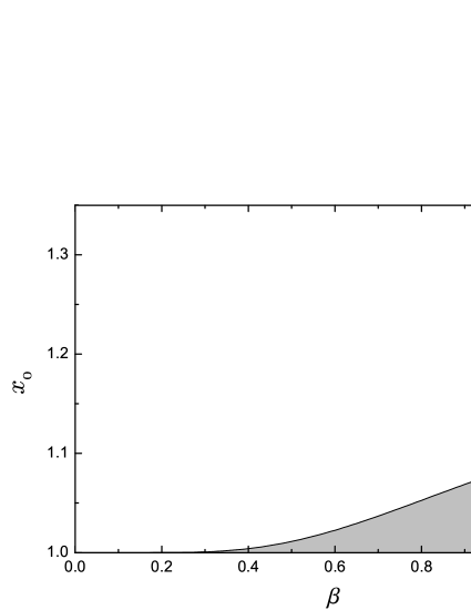
Figure 2: The light gray region corresponds to values of $(\beta,x_{0})$ which do not satisfy the dominant-energy condition, while the dark gray region is excluded by the constraint (16). The blank area corresponds to shell configurations satisfying the weak, strong and dominant energy conditions.

III Quantizing the field and awaking the vacuum

Now, let us consider a nonminimally coupled real scalar field $\Phi$ with null mass defined over a spacetime of a spheroidal shell as discussed in Sec. II (see Sec. III of Ref. llmv for a discussion about the physical reasonableness of the null-mass assumption). It will satisfy the Klein-Gordon equation

$$-\nabla_{\mu}\nabla^{\mu}\Phi+\xi R\Phi=0,$$ (31)

where $R$ is the scalar curvature and $\xi={\rm const}$ is a dimensionless parameter.

We follow the canonical quantization procedure and expand the corresponding field operator as usually:

$$\hat{\Phi}=\int d\vartheta(\eta)[\hat{a}_{\eta}u_{\eta}+\hat{a}_{\eta}^{\dagger}u_{\eta}^{*}],$$ (32)

where $\vartheta$ is a measure defined on the set of quantum numbers $\eta$. Here, $u_{\eta}$ and $u_{\eta}^{*}$ are positive and negative norm modes with respect to the Klein-Gordon inner product birrell_and_davies , respectively, satisfying Eq. (31). Then, the annihilation $\hat{a}_{\eta}$ and creation $\hat{a}_{\eta}^{\dagger}$ operators satisfy the usual commutation relations $[\hat{a}_{\alpha},\hat{a}_{\beta}^{\dagger}]=\delta(\alpha,\beta)$, $[\hat{a}_{\alpha},\hat{a}_{\beta}]=0$ and the vacuum state $|0\rangle$ is defined by requiring $\hat{a}_{\eta}|0\rangle=0$ for all $\eta$.

Since the spacetime is static and axially symmetric, it is natural to look for positive-norm modes in the form

$$u_{\eta}(t,\vec{\chi},\varphi)=T_{\sigma}(t)F_{\sigma\mu}(\vec{\chi})e^{i\mu\varphi},$$ (33)

where $\vec{\chi}=(\tilde{r},\theta)$ and $\vec{\chi}=(x,y)$ inside and outside the shell, respectively, $\mu\in\mathbb{Z}$ is the azimuthal quantum number, and $\sigma={\rm const}$. By using Eq. (33) in Eq. (31), we see that $T_{\sigma}(t)$ obeys

$$\frac{d^{2}}{dt^{2}}T_{\sigma}+\sigma T_{\sigma}=0,$$ (34)

while $F_{\sigma\mu}(\chi)$ satisfies

$$-\frac{1}{a^{2}}\left(\frac{x_{0}-1}{x_{0}+1}\right)^{2\beta}\left[\frac{1}{\tilde{r}^{2}}\partial_{\tilde{r}}(\tilde{r}^{2}\partial_{\tilde{r}})+\frac{1}{\tilde{r}^{2}\sin\theta}\partial_{\theta}(\sin\theta\partial_{\theta})\right.$$

$$-\left.\frac{\mu^{2}}{\tilde{r}^{2}\sin^{2}\theta}\right]F^{-}_{\sigma\mu}=\sigma F^{-}_{\sigma\mu}$$ (35)

and

$$-\frac{1}{a^{2}}\left(\frac{x-1}{x+1}\right)^{2\beta}\left\{\frac{(x^{2}-y^{2})^{\beta^{2}-1}}{(x^{2}-1)^{\beta^{2}}}\left\{\partial_{x}\left[(x^{2}-1)\partial_{x}\right]\right.\right.$$

$$+\left.\left.\partial_{y}\left[(1-y^{2})\partial_{y}\right]\right\}-\frac{\mu^{2}}{(x^{2}-1)(1-y^{2})}\right\}F^{+}_{\sigma\mu}=\sigma F^{+}_{\sigma\mu}.$$ (36)

Here, we have assigned labels “$-$” and “$+$” to $F_{\sigma\mu}$ in order to denote solutions valid inside and outside the shell, respectively.

The solutions of Eq. (34) will assume the following general forms:

$$T_{\sigma}(t)\to T_{\omega}(t)\propto\exp(-i\omega t),\;\;\;\omega>0,$$ (37)

for $\sigma\equiv\omega^{2}>0$ and

$$T_{\sigma}(t)\to T_{\Omega}(t)\propto e^{\Omega t-i\pi/12}+e^{-\Omega t+i\pi/12},\;\;\;\Omega>0,$$ (38)

for $\sigma\equiv-\Omega^{2}<0$, where the latter is one of the possible combinations which guarantee that $u_{\sigma}$ with $\sigma<0$ is indeed a positive-norm mode lv . Equation (37) is connected with the usual time-oscillating modes while Eq. (38) is associated with the so-called “tachyonic” modes. Tachyonic modes are responsible for an exponential growth of quantum fluctuations and, consequently, of the expectation value of the stress-energy-momentum tensor lv . (We address to Ref. llmv for more details on the canonical quantization procedure in the presence of unstable modes but it is worthwhile to emphasize at this point that tachyonic modes do not violate any causality canon.) The requirement that these modes be normalizable determines the possible negative values of $\sigma$ (if any) and, thus, the existence (or nonexistence) of tachyonic modes. One sees from Eq. (III) that tachyonic modes vanish exponentially at infinity:

$$F_{\sigma\mu}^{+}(x,y)\to F_{\Omega\mu}^{+}(x,y)\stackrel{{\scriptstyle x\to\infty}}{{\propto}}\exp(-\Omega ax).$$ (39)

Next, let us analyze Eqs. (III)-(III) in more detail. On account of Eq. (21), we have that

$$R=-8\pi T=-2\Delta K\delta(\ell).$$

Then, one sees from Eq. (31) that $F^{\pm}_{\sigma\mu}$ should join each other continuously on $\cal{S}$:

$$F^{-}_{\sigma\mu}(\tilde{r},\theta)|_{\cal{S}}=F^{+}_{\sigma\mu}(x,y)|_{\cal{S}},$$ (40)

while the first derivative of $F_{\sigma\mu}$ along the direction orthogonal to the shell will be discontinuous:

$$\Delta(dF_{\sigma\mu}/d\ell)|_{\cal{S}}=\xi\gamma(y)F_{\sigma\mu}|_{\cal{S}}.$$ (41)

Here, $\gamma(y)\equiv-2\Delta K$ and we recall that $\Delta K=4\pi(S^{0}_{\;0}+S^{2}_{\;2}+S^{3}_{\;3})$. By using Eqs. (23)-(25), we obtain

$$\gamma(y) =-\frac{2}{a}\left(\frac{x_{0}-1}{x_{0}+1}\right)^{\frac{\beta}{2}}\left(\frac{x_{0}^{2}-y^{2}}{x_{0}^{2}-1}\right)^{\frac{\beta^{2}-1}{2}}\left[\frac{\beta^{2}x_{0}-\beta+x_{0}}{x_{0}^{2}-1}\right.$$

$$+\left.\frac{x_{0}(1-\beta^{2})}{x_{0}^{2}-y^{2}}-\frac{1}{U(y)}\left(1-\frac{y^{2}(\beta^{2}-1)}{x_{0}^{2}-y^{2}}\right)-\frac{U(y)}{x_{0}^{2}-1}\right],$$ (42)

where we recall that $U(y)$ is given by Eq. (26). For the sake of convenience, we cast Eq. (41) in a more explicit form:

$$\left.\left(\frac{dx}{d\ell}\frac{\partial F^{+}_{\sigma\mu}}{\partial x}\right)\right|_{\cal{S}}-\left.\left(\frac{d\tilde{r}}{d\ell}\frac{\partial F^{-}_{\sigma\mu}}{\partial\tilde{r}}+\frac{d\theta}{d\ell}\frac{\partial F^{-}_{\sigma\mu}}{\partial\theta}\right)\right|_{\cal{S}}=\xi\gamma(y)F_{\sigma\mu}|_{\cal{S}},$$ (43)

where

$$\left.\frac{dx}{d\ell}\right|_{\cal{S}}=\frac{1}{a}\left(\frac{x_{0}-1}{x_{0}+1}\right)^{\beta/2}\left(\frac{x_{0}^{2}-y^{2}}{x_{0}^{2}-1}\right)^{(\beta^{2}-1)/2},$$ (44)

$$\left.\frac{d\tilde{r}}{d\ell}\right|_{\cal{S}}=\frac{D(y)g^{\prime}(y)}{\sqrt{1-g(y)^{2}}},$$ (45)

and

$$\left.\frac{d\theta}{d\ell}\right|_{\cal{S}}=\frac{D(y)f^{\prime}(y)}{f(y)^{2}}$$ (46)

with

$$D(y)\equiv\frac{1}{a}\left(\frac{x_{0}-1}{x_{0}+1}\right)^{\beta/2}\left[\frac{g^{\prime}(y)^{2}}{1-g(y)^{2}}+\frac{f^{\prime}(y)^{2}}{f(y)^{2}}\right]^{-1/2}.$$ (47)

In what follows, we search for the $\xi$ parameters which give rise to tachyonic modes and, hence, to the vacuum awakening effect, once the spacetime, characterized by the values of $x_{0}$, $\beta$ and $M$, is fixed. For this purpose, we must look for regular $F^{\pm}_{\sigma\mu}(\vec{\chi})$ functions with $\sigma<0$ satisfying Eqs. (III) and (III) inside and outside the shell, respectively, while respecting Eqs. (40) and (41) on the shell and vanishing exponentially at infinity [see Eq. (39)].

III.1 Spherical shells

Let us start with an analytical investigation of the conditions required by spherically-symmetric shells to allow the existence of tachyonic modes. It will be interesting in its own right and useful as a test for the reliability of the numerical code which will be used to treat more general axially-symmetric shells further.

First, we note from Eq. (28) that $a=M$ for $\beta=1$. Hence, by using the definitions $x\equiv r/M-1$ and $y\equiv\cos\theta$ in Eq. (12) and $x_{0}\equiv\mathsf{R}/M-1$ in Eq. (13), we write the external- and internal-to-the-shell line elements as

$$ds^{2}_{+}=-(1-2M/r)dt^{2}+(1-2M/r)^{-1}dr^{2}+r^{2}ds^{2}_{S}$$ (48)

and

$$ds^{2}_{-}=-(1-2M/\mathsf{R})dt^{2}+(1-2M/\mathsf{R})^{-1}M^{2}(d\tilde{r}^{2}+\tilde{r}^{2}ds^{2}_{S}),$$ (49)

respectively, where $ds^{2}_{S}=d\theta^{2}+\sin^{2}\theta d\varphi^{2}$. In terms of the internal and external coordinates, the shell is at

$$\tilde{r}=(1-2M/\mathsf{R})^{1/2}\mathsf{R}/M\;\;{\rm and}\;\;r=\mathsf{R},$$

respectively, from which we see that $\mathsf{R}$ is indeed the shell proper radius. In order to define a continuous radial coordinate on the shell, we introduce

$$r_{-}\equiv{M\tilde{r}}/{(1-2M/\mathsf{R})^{1/2}},\;\;\;r_{+}\equiv r$$

with respect to which the shell will be at $r_{\pm}=\mathsf{R}$.

Now, we note that the general solutions of Eqs. (III)-(III) can be cast in the form

$$F^{\pm}_{\sigma\mu}(r_{\pm},\theta)=\sum_{l=0}^{\infty}a_{l\mu}({\psi^{\pm}_{\sigma l}(r_{\pm})}/{r_{\pm}})P_{l}^{\mu}(\cos\theta),$$ (50)

where $a_{l\mu}={\rm const}$ and $P_{l}^{\mu}(\cos\theta)$ are associated Legendre functions of the first kind, degree $l=0,1,2\ldots$, and order $\mu=-l,-l+1,\ldots,l$. For the sake of convenience, we define the coordinates

$$\chi_{-}\equiv r_{-}/(1-2M/\mathsf{R})^{1/2},\;\;\;\chi_{+}\equiv r_{+}+2M\ln[r_{+}/(2M)-1]+D,$$

where $D={\rm const}$ is chosen such that $\chi_{-}$ and $\chi_{+}$ fit each other continuously on the shell. By using $\chi_{\pm}$, the functions $\psi_{\sigma l}^{\pm}$ will satisfy the “Schrödinger-like” equation

$$-d^{2}\psi_{\sigma l}^{\pm}/d\chi^{2}_{\pm}+V_{\textrm{eff}}^{(l,\pm)}\psi_{\sigma l}^{\pm}=\sigma\psi_{\sigma l}^{\pm}$$ (51)

with

$$V_{\textrm{eff}}^{(l,-)}=(1-2M/\mathsf{R})l(l+1)/r_{-}^{2},$$ (52)

$$V_{\textrm{eff}}^{(l,+)}=(1-2M/r_{+})(l(l+1)/r_{+}^{2}+2M/r_{+}^{3}).$$ (53)

The discontinuity of the potential across the shell is $\Delta V_{\textrm{eff}}=2M(1-2M/\mathsf{R})/\mathsf{R}^{3}.$ Although $V_{\rm eff}^{(l,\pm)}$ is positive everywhere off shell, the existence of tachyonic modes is still possible because the potential on the shell contains a delta distribution. Thus, depending on $\mathsf{R}/M,\xi$ and $l$, the effective potential will be “negative enough” to allow solutions of Eq. (51) for $\sigma<0$. This is codified in the discontinuity condition (41), which will be used later.

As a result of Eq. (50), the field-operator expansion (32) can be written in this case as

$$\hat{\Phi} =\sum_{l\mu}\int d\omega[\hat{b}_{\omega l\mu}v_{\omega l\mu}+\hat{b}_{\omega l\mu}^{\dagger}v^{*}_{\omega l\mu}]$$

$$+\sum_{l\mu\Omega}[\hat{c}_{\Omega l\mu}w_{\Omega l\mu}+\hat{c}_{\Omega l\mu}^{\dagger}w^{*}_{\Omega l\mu}],$$ (54)

where the only nonzero commutation relations between the creation and annihilation operators are

$$[\hat{b}_{\omega l\mu},\hat{b}^{\dagger}_{\omega^{\prime}l^{\prime}\mu^{\prime}}] =\delta_{ll^{\prime}}\delta_{\mu\mu^{\prime}}\delta(\omega-\omega^{\prime}),$$ (55)

$$[\hat{c}_{\Omega l\mu},\hat{c}^{\dagger}_{\Omega^{\prime}l^{\prime}\mu^{\prime}}] =\delta_{ll^{\prime}}\delta_{\mu\mu^{\prime}}\delta_{\Omega\Omega^{\prime}},$$ (56)

the modes read

$$v^{\pm}_{\omega l\mu}=T_{\omega}(t)(\psi^{\pm}_{\omega l}(r_{\pm})/r_{\pm})Y_{l\mu}(\theta,\varphi),$$ (57)

$$w^{\pm}_{\Omega l\mu}=T_{\Omega}(t)(\psi^{\pm}_{\Omega l}(r_{\pm})/r_{\pm})Y_{l\mu}(\theta,\varphi)$$ (58)

with

$$Y_{l\mu}(\theta,\varphi)\equiv\sqrt{\frac{(2l+1)(l-\mu)!}{4\pi(l+\mu)!}}P_{l}^{\mu}(\cos\theta)e^{i\mu\varphi},$$

and we have assigned labels “$\pm$” to $v_{\omega l\mu}$ and $w_{\Omega l\mu}$ to denote solutions valid inside and outside the shell, following our previous notation.

Our search for tachyonic modes equals, thus, the search for solutions $\psi^{\pm}_{\Omega l}$ of Eq. (51) with $\sigma=-\Omega^{2}<0$. The regularity requirement for the normal modes implies that at the origin

$$\lim_{\chi_{-}\to 0}\psi^{-}_{\Omega l}=0^{+},$$ (59)

where we have assumed that it approaches zero from positive values, since the Klein-Gordon inner product fixes the mode normalization up to an arbitrary multiplicative phase (which can be chosen at our convenience). By using Eq. (51) with Eq. (59), we conclude that

$$0<\psi^{-}_{\Omega l}(r_{-})|_{\cal S}=\psi^{+}_{\Omega l}(r_{+})|_{\cal S},$$ (60)

where the equality is a consequence of Eq. (40).

On the other hand, Eq. (41) implies that the first derivative of the radial function will be discontinuous on ${\cal S}$:

$$\left[\left(1-\frac{2M}{\mathsf{R}}\right)^{1/2}\frac{d(\psi^{+}_{\Omega l}(r_{+})/r_{+})}{dr_{+}}-\frac{d(\psi^{-}_{\Omega l}(r_{-})/r_{-})}{dr_{-}}\right]_{\cal S}=-2\frac{\xi}{\mathsf{R}}$$

$$\times\left(1-\frac{2M}{\mathsf{R}}\right)^{-1/2}\left(2-\frac{3M}{\mathsf{R}}-2\left(1-\frac{2M}{\mathsf{R}}\right)^{1/2}\right)\left.\frac{\psi^{-}_{\Omega l}(r_{-})}{r_{-}}\right|_{\cal S}.$$ (61)

Then, $d\psi^{+}_{\Omega l}/d\chi_{+}|_{\cal S}$ will be, in general, a nontrivial function of the field and shell parameters. Now, by noting from Eq. (51) that

$$\psi^{\pm}_{\Omega l}\gtrless 0\Rightarrow d^{2}\psi^{\pm}_{\Omega l}/d\chi_{\pm}^{2}\gtrless 0,$$

we conclude that either $\psi^{+}_{\Omega l}$ changes sign once, diverging negatively at infinity, or it remains always positive. Tachyonic modes (with $\Omega>0$) will be associated with $\psi^{\pm}_{\Omega l}>0$ with the additional requirement that

$$\lim_{\chi_{+}\to+\infty}\psi^{+}_{\Omega l}=0^{+}.$$ (62)

It follows, then, from Eq. (51) that for a given shell configuration there will exist up to one tachyonic mode for each fixed $l$.

In order to investigate which shell configurations give rise to tachyonic modes, let us first note that there always exist a negative enough $\sigma=-\Omega_{0}^{2}<0$, such that

$$\lim_{\chi_{+}\to+\infty}\psi^{+}_{\Omega_{0}l}=+\infty.$$ (63)

Then, if

$$\lim_{\chi_{+}\to+\infty}\psi^{+}_{0l}=-\infty,$$ (64)

it is certain that there will exist some $\Omega\in(0,\Omega_{0})$ satisfying condition (62). Conversely, if condition (64) is not verified, there will be no tachyonic mode.

The solutions of Eq. (51) with $\Omega=0$ satisfying Eq. (59) can be written as

$$\psi^{-}_{0l}({r_{-}})=A_{l}{r_{-}}^{l+1}/\mathsf{R}^{l},\;\;A_{l}>0,$$ (65)

$$\psi^{+}_{0l}(r_{+})=B_{l}P_{l}(r_{+}/M-1)r_{+}+C_{l}Q_{l}(r_{+}/M-1)r_{+},$$ (66)

where $A_{l},B_{l}$ and $C_{l}$ are constants. Next, by imposing conditions (60) and (61) on the shell, we obtain

$$\frac{B_{0}}{A_{0}}=1-\frac{\xi\mathsf{R}}{M}\left(\frac{3M}{\mathsf{R}}-2+2\sqrt{1-\frac{2M}{\mathsf{R}}}\right)\ln\left(1-\frac{2M}{\mathsf{R}}\right)$$ (67)

and

$$\frac{B_{l}}{A_{l}}= -\frac{[(l+4\xi)({Mx_{0}}/{\mathsf{R}}-\sqrt{1-{2M}/{\mathsf{R}}})-{2M\xi}/{\mathsf{R}}]Q_{l}(x_{0})}{({lM}/{\mathsf{R}})\left[P_{l}(x_{0})Q_{l-1}(x_{0})-P_{l-1}(x_{0})Q_{l}(x_{0})\right]}$$

$$+\frac{({lM}/{\mathsf{R}})Q_{l-1}(x_{0})}{({lM}/{\mathsf{R}})\left[P_{l}(x_{0})Q_{l-1}(x_{0})-P_{l-1}(x_{0})Q_{l}(x_{0})\right]}$$ (68)

for $l=0$ and $l\geq 1$, respectively, and

$$\frac{C_{l}}{A_{l}}=\frac{1-(B_{l}/A_{l})P_{l}(x_{0})}{Q_{l}(x_{0})}$$ (69)

for $l\geq 0$, where we recall that in the spherical case $x_{0}=\mathsf{R}/M-1$. Then, by using that

$$\lim_{r_{+}\to+\infty}Q_{l}(r_{+}/M-1)r_{+}\sim r_{+}^{-l},$$ (70)

$$\lim_{r_{+}\to+\infty}P_{l}(r_{+}/M-1)r_{+}\sim r_{+}^{l+1},$$ (71)

we see from Eq. (66) and condition (64) that the existence of tachyonic modes with some $\Omega>0$ requires $B_{l}/A_{l}<0$. ($B_{l}/A_{l}=0$ corresponds to “marginal” tachyonic modes characterized by having the quantum number $\Omega=0$.) This establishes a relationship between the field parameter $\xi$ and the shell ratio $M/\mathsf{R}$. In Figs. 3 and 4, we show the parameter-space region where tachyonic modes with $l=0$ and $l=1$ do exist, respectively. We note that because the smaller the $l$ the lower the $V_{\textrm{eff}}^{(l,\pm)}$, the existence of a tachyonic mode with $l=l_{0}$ implies the existence of tachyonic modes with $l=0,\ldots,l_{0}-1$. This can be seen in Figs. 3 and 4 as we note that the tachyonic-mode region for $l=1$ is contained in the one for $l=0$. Clearly, the existence of a single tachyonic mode is enough to induce an exponential growth of quantum fluctuations leading to the vacuum awakening effect. We note, in particular, that there are shell configurations which allow the existence of tachyonic modes for the conformal field case, $\xi=1/6$. Nevertheless, it can be also seen from Figs. 3 and 4 that for these configurations the dominant-energy condition (30) is violated.

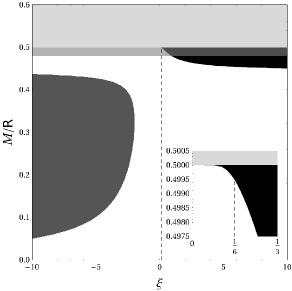
Figure 3: The black and dark-gray areas depict the parameter-space region where $B_{0}/A_{0}<0$ leading to the “vacuum awakening effect”. The magnitude of the vacuum energy density on the shell grows positively and negatively in the black and dark-gray regions, respectively (see discussion in Sec. IV). The light-gray strip is excluded from the parameter space because no static spherical shell can exist with $\mathsf{R}\leq 2M$, while the translucent-gray one contains those configurations which violate the dominant-energy condition. The inset graph emphasizes that there are shell configurations which allow the presence of tachyonic modes for $\xi=1/6$ (vertical dashed line), although the dominant-energy condition is not satisfied.

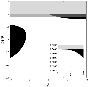
Figure 4: The black areas depict the parameter-space region where tachyonic modes with $l=1$ are present. The light- and translucent-gray regions represent the same as in Fig. 3. In contrast to the $l=0$ case, no analysis is performed here concerning whether the vacuum energy density on the shell grows positively or negatively because any contribution coming from $l=1$ is dominated by the one associated with $l=0$.

III.2 Prolate and oblate shells

Now, we proceed to treat the prolate ($0<\beta<1$) and oblate ($\beta>1$) spheroidal shell cases. Here, we shall focus our attention on the boundaries which curb the regions where the vacuum awakening effect occurs due to the existence of any tachyonic mode. These boundaries are associated with the presence of marginal tachyonic solutions with $\Omega=0$ [see discussion below Eq. (71)]. Moreover, following the spherically-symmetric case reasoning where the most likely tachyonic modes have $l=0$ (implying $\mu=0$), we will look for marginal tachyonic modes ($\Omega=0\Rightarrow\sigma=0$) with $\mu=0$ in the axially-symmetric prolate and oblate cases. Then, the relevant regular solutions of Eqs. (III) and (III) which give rise to normalizable modes are

$$F^{-}_{00}=\sum_{l}{A_{l}\tilde{r}^{l}P_{l}(\cos\theta)}$$ (72)

and

$$F^{+}_{00}=\sum_{l}{C_{l}Q_{l}(x)P_{l}(y)}.$$ (73)

We note that Eqs. (72)-(73) generalize the spherically-symmetric relation (50) with $\sigma=\mu=0$ provided that one sets $B_{l}=0$ in Eq. (66) [see observation within parentheses below Eq. (71)].

Next, we use Eqs. (72)-(73) in the continuity condition (40) to determine the $C_{l}$ coefficients in terms of the $A_{l}$ ones:

$$C_{l^{\prime}}=\frac{2l^{\prime}+1}{2Q_{l^{\prime}}(x_{0})}\sum_{l}{A_{l}\int_{-1}^{1}{dyP_{l^{\prime}}(y)f(y)^{l}P_{l}[g(y)]}},$$ (74)

where we recall that $f(y)$ and $g(y)$ are given in Eqs. (14) and (15), respectively, and we have used the orthonormality condition

$$\int_{-1}^{1}{P_{n}(y)P_{m}(y)dy}=\frac{2}{2n+1}\delta_{nm}.$$ (75)

Once we have determined Eq. (74) for $A_{l}$ and $C_{l}$ connected with the marginal tachyonic modes associated with Eqs. (72)-(73) (which satisfy the proper boundary conditions), the frontiers which curb the unstable regions are obtained as we impose the first-derivative constraint (41). Here, it is convenient to note that Eq. (41), supplied by Eqs. (72), (73), and (74), can be cast as $\sum_{l}{A_{l}G_{l}(y)}=0$ for an intricate but otherwise known function $G_{l}(y)$. By expanding $G_{l}(y)$ in terms of Legendre polynomials, Eq. (41) can be written as

$$\sum_{l}{\sum_{l^{\prime}}{A_{l}k_{ll^{\prime}}}P_{l^{\prime}}(y)}=0,$$ (76)

where $k_{ll^{\prime}}\equiv(l^{\prime}+1/2)(k^{(1)}_{ll^{\prime}}+k^{(2)}_{ll^{\prime}}+k^{(3)}_{ll^{\prime}})$ with

$$k^{(1)}_{ll^{\prime}}=\left[\frac{1}{Q_{l^{\prime}}(x)}\frac{dQ_{l^{\prime}}(x)}{dx}\right]_{x=x_{0}}\int_{-1}^{1}{dyP_{l^{\prime}}(y)f(y)^{l}P_{l}[g(y)]},$$ (77)

$$k^{(2)}_{ll^{\prime}} =-\int_{-1}^{1}{dyP_{l^{\prime}}(y)\left[\frac{dx}{d\ell}\right]^{-1}_{\cal{S}}\left\{lf(y)^{l-1}\left[\frac{d\tilde{r}}{d\ell}\right]_{\cal{S}}P_{l}[g(y)]\right.}$$

$$-\left.\frac{lf(y)^{l}}{\sqrt{1-g(y)^{2}}}\left[\frac{d\theta}{d\ell}\right]_{\cal{S}}\{-g(y)P_{l}[g(y)]+P_{l-1}[g(y)]\}\right\}$$ (78)

and

$$k^{(3)}_{ll^{\prime}}=-\xi\int_{-1}^{1}{dyP_{l^{\prime}}(y)\left[\frac{dx}{d\ell}\right]^{-1}_{\cal{S}}\gamma(y)f(y)^{l}P_{l}[g(y)]}.$$ (79)

Here, we recall that $\gamma(y)$, $dx/d\ell|_{\cal{S}}$, $d\tilde{r}/d\ell|_{\cal{S}}$, and $d\theta/d\ell|_{\cal{S}}$ are given in Eqs. (III), (44), (45), and (46), respectively. Then, by using the orthonormality property of the Legendre polynomials, Eq. (76) leads to

$$\sum_{l}{A_{l}k_{ll^{\prime}}}=0.$$ (80)

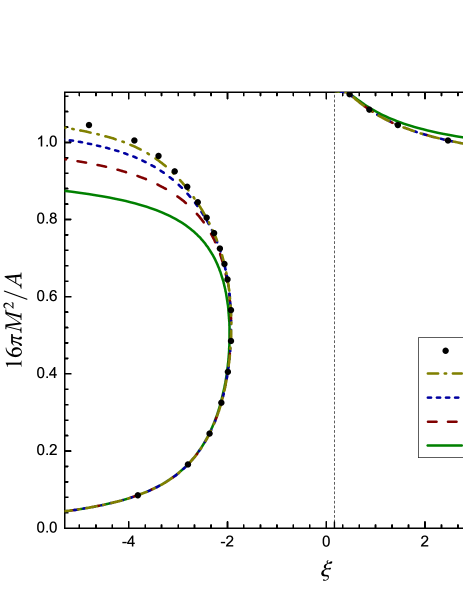
Figure 5: Diagram showing how higher order $N$ approximations converge to the actual boundaries which curb the tachyonic unstable regions for a considerably prolate shell, $n=0.25$. Configurations allowing for tachyonic modes are those to the left of the curves on the left-hand side and to the right of the curves on the right-hand side. We note that in the $16\pi M^{2}/A\ll 1$ regime, the $N=0$ approximation is already quite satisfactory in contrast to the $16\pi M^{2}/A\approx 1$ regime. For $N=8$, only few points were obtained due to the computational cost.

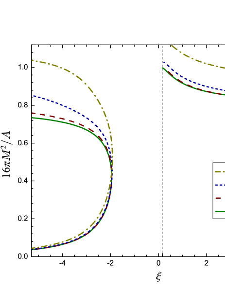
Figure 6: Diagram showing the boundaries which circumscribe the regions where the vacuum awakening effect is triggered by prolate-spheroidal shells with $n=0.25$, $0.5$ and $0.75$. The spherical ($n=1$) case is plotted for comparison. The vertical dashed line indicates the conformal-coupling value $\xi=1/6$. Configurations allowing for tachyonic modes are those to the left of the curves on the left-hand side and to the right of the curves on the right-hand side.

Let us, now, consider $k_{ll^{\prime}}$ as elements of a matrix $\mathcal{K}$. In the spherically-symmetric case, $\mathcal{K}$ is diagonal: $k_{ll^{\prime}}=g_{l}\delta_{ll^{\prime}}$ with $g_{l}$ being constants depending on the shell, $M/\mathsf{R}$, and field, $\xi,l$, parameters. The borderlines associated with the regions containing tachyonic modes for each $l$ are obtained by solving $g_{l}=0$ for $\xi$ as a function of $M/\mathsf{R}$. In the absence of spherical symmetry, the corresponding borderlines inside which tachyonic modes exist can be obtained similarly by vanishing the eigenvalues of $\mathcal{K}$. The vanishing-eigenvalue condition can be imposed on $\mathcal{K}$ by solving the corresponding characteristic equation

$$\det{\mathcal{K}}=0.$$ (81)

This will drive Eq. (80) to have a nontrivial solution for the $A_{l}$ coefficients. We recall that, eventually, all modes should be Klein-Gordon orthonormalized, which fixes any remaining $A_{l}$ left free.

For computational purposes, we truncate (the infinite matrix) $\mathcal{K}$ by imposing $0\leq l,l^{\prime}\leq N$ for a large enough $N$. This is justified since the $k_{ll^{\prime}}$ elements decrease as the values of $l$ or $l^{\prime}$ increase. By fixing the $\beta$ and $x_{0}$ parameters, Eq. (81) is expected to be satisfied by $N+1$ values of $\xi$, which corresponds in the spherical case to the fact that for a fixed $M/\mathsf{R}$ value, the boundary of the unstable regions, associated with the marginal tachyonic modes, are at different $\xi$ values; each one corresponding to a distinct $l=0,\ldots,N$ (see Figs. 3 and 4). Because in the prolate and oblate cases we are interested in the regions where the vacuum awakening effect occurs by the existence of any tachyonic mode, we shall look for the $\xi$ solutions of Eq. (81) which lead to the boundary enclosing the largest possible unstable region. (In the spherical case, it corresponds to the boundary of the black and dark-grey regions in Fig. 3 associated with $l=0$.) For relatively small deviations from sphericity, a quite reasonable approximation is already obtained by taking $N=0$. By increasing $N$, we introduce higher order corrections. These corrections are seen to be more relevant as larger deviations from sphericity are considered as can be verified in Fig. 5 for a considerably prolate shell.

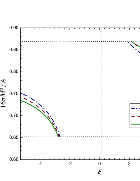
Figure 7: Diagram showing the boundaries which limit the regions where the vacuum awakening effect is triggered by an oblate-spheroidal shell with $n=1/0.85\approx 1.18$. Prolate, $n=0.85$, and spherical, $n=1$, cases are plotted, as well, for the sake of comparison (restricted to the domain of the oblate case, which is indicated by the horizontal dotted lines). The vertical dashed line indicates the conformal-coupling value $\xi=1/6$. Configurations allowing for tachyonic modes are those to the left of the curves on the left-hand side and to the right of the curves on the right-hand side.

In Figs. 6 and 7, we show the results obtained for some prolate and oblate shells, respectively, assuming $N=6$. For the sake of clarity, we have characterized the shells by their equatorial-per-meridional size ratios $n$ and proper areas $A$ as given in Eqs. (18) and (20), respectively, since they have a more straightforward physical meaning than $x_{0}$ and $\beta$. Figure 6 shows that the lines which limit the regions where the vacuum is awakened by prolate shells differ significantly from the spherical case for dense enough configurations, $16\pi M^{2}/A\approx 1$. In contrast to the spherical case, where there is no equilibrium configuration for $16\pi M^{2}/A\geq 1$, in the prolate one, $16\pi M^{2}/A$ can acquire arbitrarily large values when $n$ is arbitrarily small. Figure 7 puts in context the oblate case. We recall from Sec. II that the degree of nonsphericity for this class of solutions is restricted on account of the constraint (16): $\beta>1\Rightarrow x_{0}>\beta$, leading to $1<n\lesssim 1.3$. This restriction reflects itself on the allowed values for $16\pi M^{2}/A$. The excised regions at the top and bottom of Fig. 7 come from this condition applied to the oblate shell considered in the graph. From this figure, we also see that the oblate shell with $n=1/0.85\approx 1.18$ is more favorable to trigger the effect than the associated prolate one with $n=0.85$.

IV Exponential growth of the vacuum energy density

Finally, we investigate the exponential growth of the vacuum energy density induced by the existence of tachyonic modes. Although the vacuum energy density will be a nontrivial point-dependent function, the total vacuum energy will be time conserved lv . Let us suppose that a spheroidal shell evolves from (i) an initial static configuration $(x_{0},\beta,M)_{\textrm{in}}$ where Eq. (31) is only allowed to have time-oscillating solutions to (ii) a new static configuration $(x_{0},\beta,M)_{\textrm{out}}$ where Eq. (31) is permitted to also have tachyonic ones. Because the oscillating in-modes will eventually evolve into tachyonic and oscillating out-modes, the vacuum energy density $\langle\hat{T}_{00}\rangle\equiv\langle 0_{\rm in}|\hat{T}_{00}|0_{\rm in}\rangle$ will grow exponentially. Here, we assume the vacuum $|0_{\rm in}\rangle$ to be the no-particle state defined according to the oscillating in-modes (see, e.g., Ref. llmv for a more comprehensive discussion).

A general expression for the exponential growth of the expectation value of the stress-energy-momentum tensor was calculated in Ref. lv . By applying it to the spherical shell case, we obtain the following leading contribution to the vacuum energy density:

$$\langle\hat{T}_{00}\rangle=\langle\hat{T}^{-}_{00}\rangle H(-\ell)+\langle\hat{T}^{+}_{00}\rangle H(\ell)+\langle\hat{T}_{00}\rangle_{\cal S},$$ (82)

where we recall that $\ell$ is the proper distance along geodesics intercepting orthogonally $\cal{S}$ [as defined below Eq. (21)] and $H(\ell)$ is the Heaviside step function. Here, $\langle\hat{T}_{00}^{-}\rangle$, $\langle\hat{T}_{00}^{+}\rangle$, and $\langle\hat{T}_{00}\rangle_{\cal S}$ are the vacuum contributions to the energy density inside, outside and on the shell, respectively, where

$$\langle\hat{T}^{-}_{00}\rangle \sim\frac{\kappa}{8\pi}\frac{e^{2\bar{\Omega}t}}{r_{-}^{2}}\left(1-\frac{2M}{\mathsf{R}}\right)\frac{d}{dr_{-}}\left[\left(\frac{1-4\xi}{4\bar{\Omega}}\right)r_{-}^{2}\right.$$

$$\left.\times\frac{d(\psi^{-}_{\bar{\Omega}0}(r_{-})/r_{-})^{2}}{dr_{-}}\right],$$ (83)

$$\langle\hat{T}^{+}_{00}\rangle \sim\frac{\kappa}{8\pi}\frac{e^{2\bar{\Omega}t}}{r_{+}^{2}}\left(1-\frac{2M}{r_{+}}\right)\frac{d}{dr_{+}}\left[\left(\frac{1-4\xi}{4\bar{\Omega}}\right)r_{+}^{2}\right.$$

$$\left.\times\left(1-\frac{2M}{r_{+}}\right)\frac{d(\psi^{+}_{\bar{\Omega}0}/r_{+})^{2}}{dr_{+}}+\frac{\xi M}{{\bar{\Omega}}}(\psi^{+}_{\bar{\Omega}0}(r_{+})/{r_{+}})^{2}\right],$$ (84)

$$\langle\hat{T}_{00}\rangle_{\cal S} \sim\frac{\kappa}{8\pi}e^{2\bar{\Omega}t}\left(1-\frac{2M}{\mathsf{R}}\right)^{1/2}\frac{\xi}{\mathsf{R}}\left[(1-4\xi)\left(\frac{3M}{\mathsf{R}}-2\right.\right.$$

$$\left.\left.+2\left(1-\frac{2M}{\mathsf{R}}\right)^{1/2}\right)+\frac{M}{\mathsf{R}}\right]\frac{(\psi^{+}_{\bar{\Omega}0}(r_{+})/{r_{+}})^{2}}{\bar{\Omega}}\delta(\ell)$$ (85)

with $\kappa$ being a positive constant of order one related to the decomposition of the in-modes in terms of the out-modes and $\bar{\Omega}$ denoting the largest $\Omega$ selected from the set of all tachyonic solutions. By analyzing the factor multiplying the delta distribution in Eq. (IV), one can verify whether the vacuum contribution to the energy density is positive or negative on the shell. Our conclusions are depicted in Fig. 3: the black and dark-grey regions are associated with shell configurations where $\langle\hat{T}_{00}\rangle_{\cal S}$ grows positively and negatively, respectively. Similarly, one concludes from Eq. (IV) that the total vacuum energy inside our spherical shells is positive, null and negative when $\xi<1/4$, $\xi=1/4$, and $\xi>1/4$, respectively.

As a matter of fact, eventually the scalar field and background spacetime must evolve into some final stable configuration, where tachyonic modes are not present, in order to detain the exponential growth of the stress-energy-momentum tensor. The precise dynamical description of how the “vacuum falls asleep” again is presently under debate pcbrs11 . In spite of the quantum subtleties involved in this discussion, at some point the scalar field is expected to loose coherence after what a classical general-relativistic analysis should be suitable. The evolution of axially-symmetric rather than spherically-symmetric systems may lead to new interesting features.

V Conclusions

It was recently shown that relativistic stars are able to induce an exponential enhancement of the vacuum fluctuations for some nonminimally coupled free scalar fields. In Ref. lmv it was assumed spherical symmetry to describe compact objects, which is expected to be a very good approximation for most relativistic stars ligo . In this article, however, we were interested in analyzing how deviations from sphericity would impact on the vacuum awakening effect. For this purpose we have considered a class of axially-symmetric spheroidal shells. This has allowed us to pursue our goal, while avoiding concerns about how to model the interior spacetime of nonspherical compact sources. Fig. 6 shows that for dense enough configurations, $16\pi M^{2}/A\approx 1$, the awakening of the vacuum becomes more sensitive to prolate deviations from sphericity. Fig. 7 unveils that oblate shells with $n=n_{0}$ seem to be more efficient to awake the vacuum in comparison to prolate ones with $n=1/n_{0}$.

As a consistency check, we have performed an analytical investigation for the spherically-symmetric shell case in order to test the numerical codes used to discuss the general axially-symmetric one. It was shown, in particular, that in contrast to the relativistic stars analyzed in Ref. lmv , spherically-symmetric shells are able to awake the vacuum for conformally coupled scalar fields, $\xi=1/6$ (see Figs. 3-4). The exponential growth of the vacuum energy density was analyzed for the spherically-symmetric case in Sec. IV.

The present paper is part of a quest which aims at understanding the vacuum awakening effect in the context of physically realistic stars, where (i) deviations from sphericity, (ii) rotation, and (iii) realistic equations of state must be considered. In Ref. lmv , the authors focused on (iii), while in the present paper we have privileged (i). We are presently giving attention to (i) and (ii) by analyzing the vacuum awakening effect in the spacetime of spheroidal rotating shells mmv . The full consideration of the three aspects altogether will be necessary for a sharp prediction about what scalar fields would have their vacua awakened by realistic relativistic stars. It would be particularly interesting to see whether neutron stars would be able to awake the vacuum of minimally and conformally coupled scalar fields.

References

(1)
W. C. C. Lima and D. A. T. Vanzella,
Phys. Rev. Lett. 104, 161102 (2010).
(2)
W. C. C. Lima, G. E. A. Matsas, and D. A. T. Vanzella,
Phys. Rev. Lett. 105, 151102 (2010).
(3)
A. G. S. Landulfo, W. C. C. Lima, G. E. A. Matsas, and D. A. T. Vanzella,
Phys. Rev. D 86, 104025 (2012).
(4)
J. Novak,
Phys. Rev. D 58, 064019 (1998).
(5)
M. Ruiz, J. C. Degollado, M. Alcubierre, D. Núñez, and M. Salgado,
Phys. Rev. D 86, 104044 (2012).
(6)
J. D. McCrea,
J. Phys. A 9, 697 (1976).
(7)
W. Israel,
Nuovo Cimento 44B, 1 (1966);
V. de la Cruz and W. Israel,
Nuovo Cimento 51A, 774 (1967).
(8)
E. Poisson,
A Relativist’s Toolkit
(Cambridge University Press, Cambridge, 2004).
(9)
J. L. Synge,
Relativity: the General Theory
(North-Holland Publishing Company, Amsterdam, 1964).
(10)
M. E. Abramowitz and I. A. Stegun,
Handbook of mathematical functions
(Dover, New York, 1972).
(11)
H. Quevedo,
Phys. Rev. D 39, 2904 (1989).
(12) R. M. Wald,
General Relativity
(The University of Chicago Press, Chicago, 1984).
(13)
N. D. Birrell and P. C. W. Davies,
Quantum fields in curved space
(Cambridge University Press, Cambridge, 1982).
(14)
P. Pani, V. Cardoso, E. Berti, J. Read, and M. Salgado,
Phys. Rev. D 83, 081501 (2011).
(15)
B. P. Abbott et al.,
Astroph. J. 713, 671 (2010).
(16)
R. F. P. Mendes, G. E. A. Matsas, and D. A. T. Vanzella
(in preparation).