Dimensionless constants and cosmological measurements

Abstract

The laws of physics have a set of fundamental constants, and it is generally admitted that only dimensionless combinations of constants have physical significance. These combinations include the electromagnetic and gravitational fine structure constants, $\alpha=e^{2}/4\pi\epsilon_{0}\hbar c$ and $\alpha_{G}=Gm_{p}^{2}/\hbar c$, along with the ratios of elementary-particles masses. Cosmological measurements clearly depend on the values of these constants in the past and can therefore give information on their time dependence if the effects of time-varying constants can be separated from the effects of cosmological parameters. The latter can be eliminated by using pairs of redundant measurements and here we show how such pairs conspire to give information only on dimensionless combinations of constants. Among other possibilities, we will use distance measurements based on Baryon Acoustic Oscillations (BAO) and on type Ia supernova. The fact that measurements yield information only on dimensionless combinations is traced to the fact that distances between co-moving points expand following the same function of time that governs the redshift of photon wavelengths.

1 Introduction

Cosmological observations of high-redshift objects tell us about the conditions in the distant past and it is natural to try to use them to see if the physical laws have changed over time. One simple type of change would involve time variations of the fundamental constants (hereafter TVOFCs) [1]. The most famous searches for TVOFC are those for time variations of the fine-structure constant, $\alpha$, that are performed by looking for a redshift dependence in the splitting of atomic or molecular spectral lines. Current results using atomic fine-structure splittings give controversial evidence for [2] or against [3] such a variation at the level of $\Delta\alpha/\alpha\sim 10^{-5}$ over $\sim 10^{10}$yr. This sort of study makes use of redundant cosmological information: a spectral doublet has two lines that can be used to measure the redshift. Because the cosmological redshift is achromatic, any difference in the two redshifts could be explained by a different fundamental constants at the time when the photons were produced, leading to a splitting different from its present value.

Another suggestion for TVOFCs comes from the observed fluxes of high-redshift type-Ia supernovae (SNIa) [4, 5, 6, 7]. These events have fluxes about 40% smaller than what would be expected in a universe where the expansion was being decelerated by the ordinary gravitational attraction of a critical density of matter. The generally accepted explanation for this low flux is that the universe contains dark-energy that accelerates the expansion, causing the supernovae to be about 20% further from us (at a given redshift) than expected. An alternative explanation of the faintness of distant SNIa would be that in the past they were less luminous than those that explode now. This might be simply due to the astrophysical conditions changing over time. A more interesting possibility would be that the fundamental constants governing SNIa luminosities were different in the past. We will see that SNIa luminosities depend strongly on the gravitational constant, $G$, at the moment of the explosion. Of course $G$ also determines the expansion of the universe so the supernova flux we can expect to receive depends also on the entire history of this constant, $G(t)$, between explosion and detection. Analyses of SNIa data taking into account both supernova luminosities and light propagation have been performed [8, 9, 10, 11] yielding limits on the time variation of $G$, generally supposing that all other fundamental constants are time-independent.

The fact that one can envision both TVOFC and dark-energy interpretations of SNIa measurements illustrates the fact that a given type of observation can yield cosmological energy densities or fundamental constants but not both. This problem can be eliminated by comparing with a second distance measurement [12]. As an example, we use here measurements provided by the Baryonic Acoustic Oscillation (BAO) “standard ruler” consisting of a peak in the matter two-point correlation function at a co-moving distance of $\sim 150~{}{\rm Mpc}$. Distances to objects at a given redshift determined with BAO can be directly compared to distances deduced from the fluxes of SNIa “standard candles”. This will allow us to

• distinguish unambiguously between explanations of the low SN flux that are based on dark-energy from those based on TVOFC, or, more generally, on any physics causing ancient supernovae to be less luminous than modern ones.

and

• illustrate why only dimensionless combinations of fundamental constants can be studied with cosmological measurements.

Since it is well known that SNIa distances [6, 7] agree with BAO distances [13, 14, 15, 16], it will come as no surprise that we will not find evidence for TVOFC. Furthermore, the precision of current cosmological measurements (percent level) combined with astrophysical uncertainties will make our limits on TVOFC uncompetitive with those found by other techniques. It is therefore the second point which is the most important, i.e. placing cosmological measurements in the framework of “dimensionless cosmology” [19]. The way that pairs of measurements conspire to yield only information on dimensionless combinations will turn out to be simple but not entirely trivial: the BAO ruler expands with time in the same way as photon wavelengths. In other words, both the BAO ruler and photon wavelengths were smaller in the past by the same factor $(1+z)$ where $z$ is the redshift. To the extent that physics respects this rule, we will be condemned to study only dimensionless combinations of constants, a fact that may come as an embarrassment for advocates of non-standard theories where, for example, the speed of light is allowed to vary with time [20].

For measurements performed over a short period of time, the fact that only dimensionless combinations influence measurements follows from simple dimensionless analysis [21, 22, 23]. For example, if we measure the speed of light by measuring the time for a photon to travel the length of a rigid rod, we actually measure the number, $N_{t}$, of periods of some standard clock required for the trip. If we use an atomic clock, the period will be a well-defined function of fundamental constants. The length of the rod is some number, $N_{x}$, of inter-atomic spacings and this spacing can be assumed to depend on the fundamental constants in the same ways as the Bohr radius, $a_{B}=\hbar/\alpha m_{e}c$, being the only length formed from the relevant constants $(\hbar,e,m_{e})$ [22]. Before the measurement is performed, the only meaningful question we can ask is what will $N_{x}/N_{T}$ turn out to be? Being dimensionless itself, $N_{x}/N_{T}$ can then only depend on a dimensionless combination of fundamental constants. For example, the use of a hydrogen maser as a clock gives $N_{T}/N_{x}\propto g\alpha^{3}(m_{e}/m_{p})$ where $g$ is the electron gyromagnetic ratio, and $m_{e}$ and $m_{p}$ are the electron and proton masses.

Similarly it can be shown [23] that local measurements of the stability of planetary orbits are sensitive not to time variations of $G$ but rather to those of the “gravitational fine-structure constant”

$$\alpha_{G}=\frac{Gm_{p}^{2}}{\hbar c}=5.9\times 10^{-39}$$ (1)

In particular, monitoring orbital parameters with a radar and atomic clock give limits on the time variation of $\alpha_{G}g\alpha^{4}(m_{e}/m_{p})$.

These two examples illustrate how the effect of fundamental constants on local measurements comes both through the phenomenon being observed and through the measurement apparatus. The two effects combine to give sensitivity only to dimensionless combinations. Showing that cosmological measurements depend only on dimensionless fundamental constants is more delicate because they are much more complicated than the above examples. Care must be taken to model the influence of fundamental constants on all relevant aspects: the astrophysical phenomenon to be observed, the propagation of photons from the source to observer, and the act of observation. In what follows, we will show how dimensionality enters into two fundamental types of cosmological measurements, those of distances and of expansion rates

2 Distances

2.1 Type Ia Supernovae

The most precise method for measuring distances to galaxies is to measure the photon flux from a type Ia supernova in the galaxy. We therefore start by discussing how the fundamental constants enter SNIa observations. The production of visible light in SNIa is believed to be due to the energy released in the beta decays of the ${\rm{}^{56}Ni}$ produced in the nuclear reactions that drive the explosion. The amount of ${\rm{}^{56}Ni}$ is of order the Chandrasekhar mass which, apart from factors of order unity related to the relative numbers of neutrons and protons in the pre-explosion star, is given by

$$M_{\rm ch}\sim\alpha_{G}^{-3/2}m_{p}\sim 2.2\times 10^{57}m_{p}$$ (2)

The total energy available for visible photon production is then the number of nickel nuclei times the energy release per decay:

$$Q_{\rm SN}\sim\frac{1}{56\alpha_{G}^{3/2}}\times Q_{\rm Ni}$$ (3)

where $Q_{\rm Ni}$ is the energy release in the beta decay sequence ${\rm{}^{56}Ni}$ ${\rm\rightarrow^{56}Co}$ ${\rm\rightarrow^{56}Fe}$ , a quantity that depends of the neutron-proton mass difference and the relative binding energies of ${\rm{}^{56}Ni}$, ${\rm{}^{56}Co}$ and ${\rm{}^{56}Fe}$. Presumably, $Q_{\rm Ni}$ is determined by the relevant fundamental constants, $\Lambda_{\rm QCD}$, $\alpha$, and quark masses. It is not presently possible to give a useful formula for $Q_{\rm Ni}$ (see [1, 24] for a discussion of the problem of calculating nuclear masses). Nevertheless, in this paper we will treat $Q_{\rm Ni}$ as a name for some unknown combination of fundamental constants with the dimension of energy. We then write $Q_{\rm SN}$ in a way that allows for TVOFC:

$$Q_{\rm SN}(t_{1})\sim\frac{Q_{\rm Ni}(t_{1})}{56\alpha_{G}^{3/2}(t_{1})}$$ (4)

Throughout this paper, $t_{1}$ will be the time of production of the photons that we observe later at $t_{0}$. We generally show the argument $t_{1}$ only for quantities that are not expected to have any time dependence. For things things that are expected to vary with time, like the expansion rate $H(z)$, we generally use the redshift $z$ as the time parameter.

It is important to admit that equation 4 is a simplification that does not do justice to the astrophysics that determines SNIa luminosities. The fact that the brightest and dimmest SNIa have luminosities differing by a factor $\sim 3$ demonstrates this unfortunate fact. This factor $\sim 3$ is reduced to an effective $Q_{\rm SN}$ dispersion of $\sim 12\%$ by using the observed durations and colors of the supernovae (via the parameters $\alpha$ and $\beta$ in [6]). In spite of these “real world” issues we use (4) as the “leading order” effect of the fundamental constants on SNIa luminosities. A lack of redshift evolution in the luminosity could then with some confidence be taken as evidence for the time-independence of $Q_{\rm Ni}/\alpha_{G}^{3/2}$ multiplied by the factors that make it dimensionless (see below). Obviously, such evidence would only be as good as our understanding of the astrophysics.

2.2 Supernova in a box

To see how the constants impact on supernova measurements, we now need to model light propagation and the detection process. Before considering cosmological measurements, we first consider a “laboratory” supernova where the progenitor is placed in an enormous cubic box that is able to resist the explosion. The box, of volume $a^{3}$ has perfectly reflecting walls so the photons emitted by the supernova are confined. Later, the photons are counted and their wavelengths measured. The total energy of the photons at the time of measurement ($t_{0}$) is

$$E_{meas}=(hc)_{t_{0}}\left\langle\frac{1}{\tilde{\lambda}_{\rm SN}}\right\rangle\tilde{N}_{\gamma}$$ (5)

where $\tilde{N}_{\gamma}$ and $\langle 1/\tilde{\lambda}_{\rm SN}\rangle$ are the number of photons and their mean inverse wavelength. Here, and throughout this paper, quantities with a tilde are quantities measured at $t_{0}$.

If we consider the possibility of time-dependent fundamental constants, we can’t assume that the size of the box is time-independent. If the changes are slow, this would cause the wavelengths of photons to be adiabatically dilated by a factor $a(t_{0})/a(t_{1})$, corresponding to a redshift, $z=a(t_{0})/a(t_{1})-1$. If the box is constructed from solid material with a time-independent number of atoms, then the size of the box is proportional to the mean inter-atomic spacing. If the box is small enough to neglect gravitational tidal distortions, it would be expected to have roughly the same dependence on the fundamental constants as the Bohr radius, $a_{B}=\hbar/(\alpha m_{e}c)$. We therefore write

$$\frac{a(t_{1})}{a(t_{0})}=\frac{a_{B}(t_{1})}{a_{B}(t_{0})}=\frac{(\hbar/\alpha m_{e}c)_{t_{1}}}{(\hbar/\alpha m_{e}c)_{t_{0}}}$$ (6)

We can then deduce $Q_{\rm SN}$ by modifying $E_{meas}$ to account for the evolution of wavelengths and $hc$:

$$Q_{\rm SN}(t_{1})=(hc)_{t_{1}}\frac{a_{B}(t_{0})}{a_{B}(t_{1})}\left\langle\frac{1}{\tilde{\lambda}_{\rm SN}}\right\rangle\tilde{N}_{\gamma}=2\pi(\alpha m_{e}c^{2})_{t_{1}}a_{B}(t_{0})\left\langle\frac{1}{\tilde{\lambda}_{\rm SN}}\right\rangle\tilde{N}_{\gamma}$$ (7)

It is more instructive to write this equation as follows

$$\left(\frac{Q_{\rm SN}}{\alpha m_{e}c^{2}}\right)_{t_{1}}\;=\;\left\langle\frac{2\pi}{\tilde{\lambda}_{\rm SN}/a_{B}(t_{0})}\right\rangle\tilde{N}_{\gamma}$$ (8)

The structure of this equation is very simple. The l.h.s. is a dimensionless quantity that depends only on fundamental constants at the moment of the explosion, via equation 4. The r.h.s. is a product of a number of photons (counted at $t_{0}$) and the dimensionless ratio of wavelengths ($\tilde{\lambda}_{\rm SN}$) and a length standard ($a_{B}$) all measured at $t_{0}$. Measuring the r.h.s. for supernovas of different explosion times then allows one to study the time evolution of the dimensionless combination of fundamental constants given by $Q_{\rm Ni}/\alpha_{G}^{3/2}\alpha m_{e}c^{2}$. In fact, comparing directly the wavelengths of the two supernova that exploded at times $t_{1}$ and $t_{2}$ and both detected at $t_{0}$ eliminates the need to measure them in units of $a_{B}$.

$$\frac{\left(Q_{\rm Ni}/\alpha_{G}^{3/2}\alpha m_{e}c^{2}\right)_{t_{1}}}{\left(Q_{\rm Ni}/\alpha_{G}^{3/2}\alpha m_{e}c^{2}\right)_{t_{2}}}=\frac{\tilde{N}_{\gamma}(1)\langle 1/\tilde{\lambda}_{\rm SN}(1)\rangle}{\tilde{N}_{\gamma}(2)\langle 1/\tilde{\lambda}_{\rm SN}(2)\rangle}$$ (9)

where the arguments $(1)$ and $(2)$ of the tilded quantities on the r.h.s. refer to the measured values for the two supernovae.

Note that the reason we ended up being sensitive to dimensionless constants at a given time comes from the fact that we assumed that $a(t)$ tracks a combination of fundamental constants, that necessarily has the dimension of length and whose form is determined by the “experimental” apparatus. In particular we assumed $a(t)\propto a_{B}(t)$. If we had supposed $a(t)\propto 1/a_{B}(t)$, equation 8 would have become

$$\left(\frac{Q_{\rm SN}}{\hbar ca_{B}}\right)_{t_{1}}\;=\;a_{B}(t_{0})^{-1}\left\langle\frac{2\pi}{\tilde{\lambda}_{\rm SN}}\right\rangle\tilde{N}_{\gamma}\hskip 14.22636pt!!$$ (10)

The quantity on l.h.s. is a dimensionful combination of fundamental constants evaluated at $t_{1}$ (!). Taking the ratio of the r.h.s. for two SNIa of different $t_{1}$ but the same $t_{0}$ would then allow us to follow the time evolution of the dimensionful combination on the l.h.s. But writing $a(t)\propto 1/a_{B}(t)$ requires us to define a new fundamental constant $a_{C}$ (dimension of length) so that $a(t)=a_{C}^{2}/a_{B}(t)$. Allowing for time variations of $a_{C}$ and defining $a_{D}(t)=a_{C}(t)^{2}/a_{B}(t)$ brings us back to the dimensionally correct form (8) but with $a_{B}$ replaced by $a_{D}$. We end up being only sensitive to the dimensionless quantity, $Q_{\rm SN}a_{D}/\hbar c$.

There is a second way to compare the two laboratory supernovas that does not make any assumptions about the behavior of the box, and is therefore more directly applicable to cosmological observations. This method compares supernova photon wavelengths with the wavelengths of a known spectral line with the same redshift. For example, we can use the Ly$\alpha\;$photons ($\lambda_{\rm Ly\alpha}=h/(3/4)\alpha^{2}m_{e}c$) that are in principle identifiable in the spectrum of the supernova or its host galaxy. If they are measured at $t_{0}$ to have wavelength $\tilde{\lambda}_{\rm Ly\alpha}(z)$, we find

$$Q_{\rm SN}(t_{1})=\tilde{N}_{\gamma}\left\langle\frac{\tilde{\lambda}_{\rm Ly\alpha}(z)}{\tilde{\lambda}_{\rm SN}}\right\rangle\left[(3/4)\alpha^{2}m_{e}c^{2}\right]_{t_{1}}$$ (11)

It is better to write this in the form

$$\left(\frac{Q_{\rm SN}}{(3/4)\alpha^{2}m_{e}c^{2}}\right)_{t_{1}}\;=\;\tilde{N}_{\gamma}\left\langle\frac{\tilde{\lambda}_{\rm Ly\alpha}(z)}{\tilde{\lambda}_{\rm SN}}\right\rangle$$ (12)

The combination of fundamental constants on the l.h.s. is the total number of supernova photons that would be produced if they were all Ly$\alpha\;$photons. The factor in $\langle\;\rangle$ on the r.h.s. corrects for the fact that they are not.

Equation 12 shows that by self-calibrating the detector with the SN Ly$\alpha\;$photons, we find that rather than measuring $Q_{\rm SN}$, we measure the dimensionless quantity $Q_{\rm SN}/\alpha^{2}m_{e}c^{2}$. By comparing such measurements from supernovae at different ages, we can determine the time evolution of $Q_{\rm Ni}/\alpha_{G}^{3/2}\alpha^{2}m_{e}c^{2}$. One should note that the use of some other photon spectral line might make one sensitive to a different combinations of fundamental constants. We use the Ly$\alpha\;$as an illustration because atomic energy levels generally have $E\propto\alpha^{2}m_{e}c^{2}$ with a constant of proportionality depending on the details of the atomic shell structure. As such, redshift determinations using any atomic transition between states of differing principle quantum number would give limits on $Q_{\rm Ni}/\alpha_{G}^{3/2}\alpha^{2}m_{e}c^{2}$.

The l.h.s.’s of equations 8 and 12 differ by a factor of $\alpha$ so comparing results from the two methods can give a direct determination of the time dependence of $\alpha$. One could also do this more directly by simply producing Ly$\alpha\;$photons at $t_{1}$, storing them in a solid box of dimension $a$, and then comparing them later at time $t_{0}$ with new Ly$\alpha\;$photons created at $t_{0}$.

2.3 Cosmological supernovae

We now attack real cosmological observations. Unlike the case of laboratory supernovae, we cannot count all ($N_{\gamma}$) photons. We count only the $\tilde{N}_{\gamma}$ photons that pass through a detector of area $A_{\rm det}$:

$$\tilde{N}_{\gamma}\,=\,N_{\gamma}\,\frac{A_{\rm det}}{A(z)}$$ (13)

where $A(z)$ is the surface area of the sphere centered on the point of the explosion and intersecting us at $t_{0}$, i.e. the size of the detector that would be needed to detect all of the photons (figure 1). $A(z)$ is related to the usual “luminosity distance”:

$$4\pi d_{L}(z)^{2}=(1+z)^{2}A(z)$$ (14)

where the two factors of $(1+z)$ account for the redshift of individual photons and cosmological time dilation.

Figure 1: The universe at the time, $t_{0}$, when an observer detects the photons from a supernova at redshift $z$. The figure shows the surface of two spherical shells, one centered on the supernova debris and the other on the observer. The surface area of the first, $A(z)$, determines the fraction of the photons detected by the observer using a detector of area $A_{\rm det}$. The surface area of the second is $4\pi r_{s}^{2}/\Delta\tilde{\theta}_{\rm B}^{2}$ where $\Delta\tilde{\theta}_{\rm B}$ is the angle on the sky of the BAO standard ruler of length $r_{s}$. For a homogeneous universe, the two areas are equal. Note that at the time of the explosion, $t_{1}$, the BAO ruler length was smaller by the same factor as the sphere’s radius, so the subtended angle does not change.

As for laboratory supernovae, the total number of photons is $Q_{\rm SN}/(3/4)\alpha^{2}m_{e}c^{2}$, evaluated at $t_{1}$ and corrected for the fact that the mean photon energy is not equal to that of a Ly$\alpha\;$photon. Equation 13 then becomes

$$\tilde{N}_{\gamma}\,=\,\left(\frac{Q_{\rm SN}}{(3/4)\alpha^{2}m_{e}c^{2}}\right)_{t_{1}}\left\langle\frac{\tilde{\lambda}_{\rm Ly\alpha}(z)}{\tilde{\lambda}_{\rm SN}}\right\rangle^{-1}\,\frac{A_{\rm det}}{A(z)}$$ (15)

or equivalently

$$A(z)\,=\,A_{\rm det}\left(\frac{Q_{\rm SN}}{(3/4)\alpha^{2}m_{e}c^{2}}\right)_{t_{1}}\left[\left\langle\frac{\tilde{\lambda}_{\rm Ly\alpha}(z)}{\tilde{\lambda}_{\rm SN}(z)}\right\rangle\right]^{-1}\,\tilde{N}_{\gamma}^{-1}$$ (16)

This is equivalent to the standard relation between $Q_{\rm SN}$, the photon flux, and the luminosity distance.

Before going on to BAO, we write equation 16 in terms of the “published” areas, $A_{\rm SN0}(z)$, that are derived from SNIa fluxes assuming no TVOFC that would lead to a spurious redshift dependence of $Q_{\rm SN}$:

$$A(z)=A_{\rm SN0}(z)\frac{\left[Q_{\rm Ni}/(\alpha_{G}^{3/2}\alpha^{2}m_{e}c^{2})\right]_{t_{1}}}{\left[Q_{\rm Ni}/(\alpha_{G}^{3/2}\alpha^{2}m_{e}c^{2})\right]_{t_{0}}}$$ (17)

Again, we assume that the primary dependence of $Q_{\rm SN}$ on the fundamental constants is contained in the simple formula (4).

2.4 BAO

Baryon Acoustic Oscillations took place before electron-proton recombination (redshifts $z>z_{rec}\sim 1070$) when the universe supported acoustic waves in the electron-proton-photon plasma. This plasma was a nearly perfect fluid because of Compton scattering of the photons on the free electrons. Sound waves propagating out of initial perturbations had the effect of separating the baryon-electron-photon component from the cold-dark-matter component which, being collisionless, did not generate waves. This separation is seen now as an enhancement in the two-point matter correlation function at a (co-moving) distance equal to the the “sound horizon”, i.e., the distance that a sound wave could travel between the big-bang and recombination

$$r_{s}\,=\int_{z_{rec}}^{\infty}\frac{c_{s}(z)dz}{H(z)}\,\sim 150~{}{\rm Mpc}$$ (18)

Here, $H(z)$ is the expansion rate and $c_{s}(z)$ is the speed of sound. The excess correlation at this distance is “co-moving” in the sense that the physical distance expands with the Universe. This means that the excess correlation is for points separated by $r_{s}/(1+z)$ where $z$ is the redshift. This expansion of the BAO ruler by the factor $1+z$ is expected to be precise at the 1% level. We will not need to know the actual value of $r_{s}$ since it will cancel out in applications for TVOFC.

Seen on the sky, the distance of enhanced correlations corresponds to angular separations and redshift separations of

$$\Delta\tilde{\theta}_{\rm B}\,=\,\frac{r_{s}}{D(z)}\hskip 28.45274pt\Delta\tilde{z}_{\rm B}\,=\,r_{s}H(z)$$ (19)

where $D(z)$ is the co-moving angular distance to the redshift $z$ (equal to the usual angular distance, $D_{A}(z)$, multiplied by $(1+z)$) and $H(z)$ is the expansion rate at redshift $z$. The first relation is the simple geometric relation illustrated in figure 1. The second is a bit more subtle and we will derive in later (equation 31).

The angular BAO effect gives a relation between the angular separation, $\Delta\tilde{\theta}$ on the sky of two points at a common redshift $z$ and the physical distance, $d$, between the two points (at the moment of observation):

$$d=r_{s}\frac{\Delta\tilde{\theta}}{\Delta\tilde{\theta}_{\rm B}(z)}$$ (20)

This gives the area of the sphere surrounding us and intersecting the supernova debris:

$$A(z)=\frac{4\pi r_{s}^{2}}{\Delta\tilde{\theta}_{\rm B}(z)^{2}}$$ (21)

As figure 1 shows, this is not the same sphere as the one that determines the supernova flux but in a homogeneous universe their surface areas must be the same, because they have the same radius. The equivalence of the two areas in a homogeneous universe is a special case of the more general relation between luminosity and angular distances, $d_{L}(z)=(1+z)^{2}d_{A}(z)$ [25].

Equation 21 has the same structure of equation 16 except that there is no (dimensionless) combination of fundamental constants. We note that the dimensioning role of $A_{\rm det}$ for supernovae as been taken by $r_{s}^{2}$ for BAO.

For the time being, there are only four published BAO measurements of $A(z)$ [13, 14, 15, 16] based on the correlation function of galaxies. They are shown in figure 2 along with individual SNIa measurements of $A(z)$ taken from [6]. There is also a new BAO measurement of $A(z=2.3)$ using the flux correlation function in the Ly$\alpha$ forest [17] but this is at too high a redshift to be compared directly with SNIa measurements.

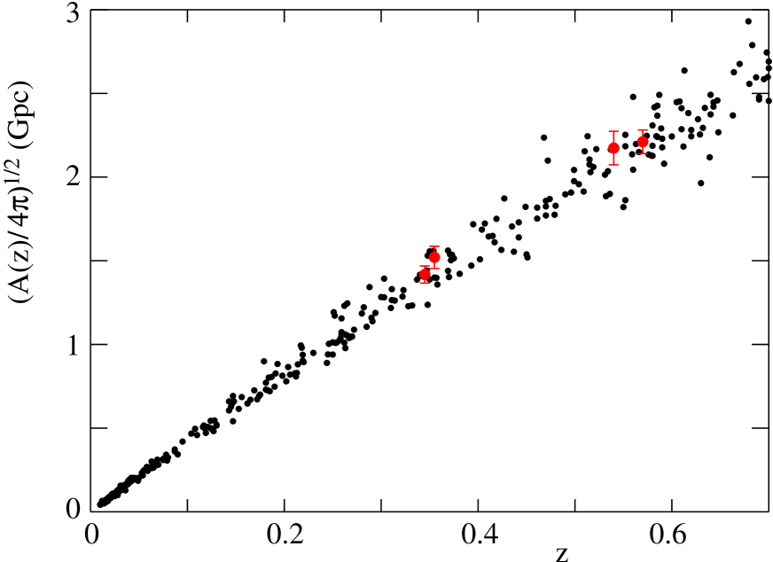
Figure 2: Measurements of $A(z)\,vs.\,z$. The black dots are individual SNIa from the compilation of [6]. The red dots are BAO measurements at $z=0.35$ [13, 15], $z=0.54$ [14]. and $z=0.57$ [16]. The BAO measurements assume $r_{s}=152{\rm Mpc}$. The supernovae distances are normalized so that $H_{0}=70~{}{\rm km\,s^{-1}Mpc^{-1}}$ and use the stretch and color parameters $\alpha=1.4$ and $\beta=3.15$.

2.5 Comparing two distance measurements

To set limits on time variations of fundamental constants we need only equate the area measurement using SNIa (equation 17) with that from BAO (equation 21):

$$\frac{4\pi r_{s}^{2}}{\Delta\tilde{\theta}_{\rm B}(z)^{2}}\,=\,A_{\rm SN0}(z)\frac{\left[Q_{\rm Ni}/(\alpha_{G}^{3/2}\alpha^{2}m_{e}c^{2})\right]_{t_{1}}}{\left[Q_{\rm Ni}/(\alpha_{G}^{3/2}\alpha^{2}m_{e}c^{2})\right]_{t_{0}}}$$ (22)

If the BAO $A(z)$ on the l.h.s. is equal to $A_{\rm SN0}(z)$ on the r.h.s. we could conclude that $Q_{\rm Ni}/(\alpha_{G}^{3/2}\alpha^{2}m_{e}c^{2})$ has not varied significantly between $t_{1}$ and $t_{0}$. Such a conclusion based on the BAO and SNIa data in figure 2 would, however, depend on the “normalization” of the BAO and SNIa distances. For the BAO, this amounts to using the value of $r_{s}$ derived from CMB data. For the SNIa data, it requires knowledge of the absolute value of the mean $Q_{\rm SN}$ or, equivalently, knowledge of the Hubble constant. (The Hubble constant, $H_{0}$, can be used to normalize the distances since for $z\ll 1$ we must have $A(z)=4\pi(zc/H_{0})^{2}$.) It is safer to eliminate the dependence on BAO and SNIa normalizations by taking ratios of $A(z)$ at different redshifts. For the BAO measurements we find

$$\frac{A(z=0.57)}{A(z=0.35)}=2.26\pm 0.26\;\hskip 14.22636pt{\rm BAO}.$$ (23)

Averaging the SNIa data over the redshift ranges $0.3<z<0.4$ and $0.51<z<0.61$ gives

$$\frac{A_{\rm SN0}(z=0.57)}{A_{\rm SN0}(z=0.35)}\,=2.40\pm 0.10\;\hskip 14.22636pt{\rm SNIa}.$$ (24)

Injecting these two results into (22) we find

$$\frac{\left[Q_{\rm Ni}/(\alpha_{G}^{3/2}\alpha^{2}m_{e}c^{2})\right]_{t(z=0.57)}}{\left[Q_{\rm Ni}/(\alpha_{G}^{3/2}\alpha^{2}m_{e}c^{2})\right]_{t(z=0.35)}}\,=\,0.94\pm 0.12$$ (25)

i.e. less than $\sim 10\%$ variation between the two redshifts. The time interval between $z=0.57$ and $z=0.35$ is $\sim 1.5\times 10^{9}~{}{\rm yr}$ for the standard cosmological parameters. The upper limit on the logarithmic time derivative of $Q_{\rm Ni}/(\alpha_{G}^{3/2}\alpha^{2}m_{e}c^{2})$ is therefore $\sim 10^{-10}{\rm yr^{-1}}$. This is considerably weaker than other published limits on TVOFC. For example, limits on $\dot{G}/G$ from lunar ranging data are in the range $\sim 10^{-12}{\rm yr^{-1}}$ [26]. Our effort has, however, given us the satisfaction of having a limit on a dimensionless combination of constants that includes, to first order, all the essential physics. Our limit also refers to time variations at a different mean time and in different regions of space than the lunar-ranging limit.

2.6 Fundamental rulers

It is instructive to replace the BAO standard ruler (whose size expands with the universe) with a hypothetical solid ruler whose length is some known number, $\tilde{N}_{x}$, times the Bohr radius. In this case, the area of equation 21 is replaced with

$$A(z)=\frac{4\pi(\tilde{N}_{x}a_{B}(t_{1}))^{2}}{\tilde{\theta}_{x}(z)^{2}}(1+z)^{2}$$ (26)

where $\tilde{\theta}_{x}$ is the observed angle subtended by the ruler on the sky. Two things are important: first we use $a_{B}(t_{1})$ instead of $a_{B}(t_{0})$ because it is the ruler’s size when it emits photons that determines it’s angle on the sky. Second, compared to (21) we have two factors of $(1+z)$ that reflect the increase in the area of the sphere’s surface between $t_{1}$ and $t_{0}$.

The redshift is given by the ratio between emitted and received Ly$\alpha\;$photons

$$1+z=\frac{\tilde{\lambda}_{\rm Ly\alpha}(z)}{[h/(3/4)\alpha^{2}m_{e}c]_{t_{1}}}$$ (27)

This gives

$$A(z)\,=\,\tilde{\lambda}_{\rm Ly\alpha}^{2}(z)\,\frac{\tilde{N}_{x}^{2}}{\tilde{\theta}_{x}(z)^{2}}\,\alpha(t_{1})^{2}\;\frac{9}{16\pi}\,$$ (28)

This now has the same dimensional structure as equations 21 and 16: products of local measurables (with a total dimension of length-squared) with a dimensionless combination of fundamental constants at $t_{1}$. Comparing areas measured with (28) with those measured with (21) would allow one to study the time dependence of $\alpha$. Comparing them with the SN-derived area (16) would allow one to study the time dependence of the dimensionless combination $Q_{\rm Ni}/\alpha_{G}^{3/2}\alpha^{4}m_{e}c^{2}$.

2.7 Why only dimensionless combinations?

We now have three measurements of $A(z)$ using standard candles (equation 16), co-moving standard rulers (21) and fixed standard rulers (28). For all three, the area depends on a dimensionless combination of fundamental constants at $t_{1}$. Taking the ratio of any two measurements of $A(z)$ then allows us to follow the time evolution of a dimensionless combination. Why is this? Why, for instance, didn’t we find a method that gives the dimensionally correct area

$$A(z)=\frac{4\pi\tilde{N}_{x}^{2}}{\tilde{\theta}_{x}(z)^{2}}a_{B}^{2}(t_{1})\hskip 14.22636pt!!$$ (29)

i.e. equation 26 without the two factors of $(1+z)$. Taking the ratio of this area with any of the other three would allow us to track the time evolution of a dimensionful quantity proportional to $a_{B}^{2}$.

While (29) is dimensionally correct, it makes no physical sense because it does not take into account the expansion of the universe. The three correct methods of measuring $A(z)$ all do this in their own way, leading to sensitivity to a dimensionless combination. For standard candles, the dimensional factor for $A(z)$ is given by $A_{\rm det}$. The fundamental constants only enter because they determine the (dimensionless) number of photons produced through the dimensionless combination $Q_{\rm SN}/\alpha^{2}m_{e}c^{2}$. This number is then corrected by the factor $\tilde{\lambda}_{\rm Ly\alpha}/\langle\tilde{\lambda}\rangle$ which assumes that all photon wavelengths evolve with the same scale factor

For the two methods using standard rulers, the dimensional factor for $A(z)$ is the square of the ruler length. More precisely, it is the ruler length at $t_{1}$ (which determines the angular size of the ruler) scaled up by a factor $(1+z)$ to take into account expansion between $t_{1}$ and $t_{0}$. For the BAO co-moving ruler and the solid ruler the length factors are

$$\frac{r_{s}}{1+z}\times(1+z)\hskip 28.45274pta_{B}(t_{1})(1+z)$$ (30)

For co-moving rulers, the factors of $(1+z)$ cancel and we end up with $A(z)$ being independent of the fundamental constants, i.e. dependent on a particularly simple dimensionless combination. For fixed rulers, the assumption that the expansion factor $1+z$ is given by a spectroscopic redshift given by equation 27 allows us to shift the dimensionality from $a_{B}(t_{1})$ to the measured $\tilde{\lambda}_{\rm Ly\alpha}$, leaving us sensitive to a dimensionless combination of constants evaluated at $t_{1}$.

The fact that the ratio of areas given by any combination of two methods thus depends on the existence of a unique scale factor that governs the expansion of all photon wavelengths as well as the distances between co-moving points.

3 The expansion rate

We now discuss measurements of TVOFC using the expansion rate at a redshift $z$. Again, we expect to be sensitive only to dimensionless combinations of constants, but, as usual, it is not obvious how this comes about.

Figure 3: Two points in the same direction on the sky that are seen by the observer to have Ly$\alpha\;$emission at $\tilde{\lambda}_{\rm Ly\alpha}$ and $\tilde{\lambda}_{\rm Ly\alpha}+\Delta\tilde{\lambda}_{\rm B}$. An observer at the point $\tilde{\lambda}_{\rm Ly\alpha}$ will see photons emerging from the point $\tilde{\lambda}_{\rm Ly\alpha}+\Delta\tilde{\lambda}_{\rm B}$ Doppler shifted by $\Delta\tilde{\lambda}_{\rm B}/\tilde{\lambda}_{\rm Ly\alpha}$. At the time, $t_{1}$, of emission of the photons seen by the observer, the two points are separated by a distance $r_{s}/(1+z)$. Hubble’s law then implies an expansion rate given by equation (31).

Other than $z=0$ measurements of $H_{0}$, the most direct measurements [13, 15, 16, 17, 18] use the BAO peak in the radial (redshift) direction. For galaxies, we will use as a radial coordinate the wavelength of its Ly$\alpha\;$photons, $\tilde{\lambda}_{\rm Ly\alpha}$, related to the redshift via equation 27. Neglecting proper motions, $\tilde{\lambda}_{\rm Ly\alpha}$ increases monotonically with distance from the observer, as illustrated in figure 3. The mass correlation function plotted in this variable has a peak at $\tilde{\lambda}_{\rm Ly\alpha}$ separations equal to $\Delta\tilde{\lambda}_{\rm B}$, corresponding to the co-moving sonic horizon, $r_{s}/(1+z)$. The wavelength separation of the BAO peak is related to the expansion rate, $H(z)$ that would be measured by an observer at that redshift:

$$H(z)=\frac{c(t_{1})\Delta\tilde{\lambda}_{\rm B}(z)/\tilde{\lambda}_{\rm Ly\alpha}(z)}{r_{s}/(1+z)}$$ (31)

To understand this relation, we note that the numerator of the r.h.s. is the Doppler shift that an observer at the point $\tilde{\lambda}_{\rm Ly\alpha}$ would see for the photons coming from the point $\tilde{\lambda}_{\rm Ly\alpha}+\Delta\tilde{\lambda}_{\rm B}$. The denominator is the distance between the two points. By Hubble’s law, the ratio gives the expansion rate, i.e. $H(z)$ on the l.h.s.

Using (27) we get

$$H(z)=\frac{\Delta\tilde{\lambda}_{\rm B}(z)}{r_{s}}\left(\frac{(3/4)\alpha^{2}m_{e}c^{2}}{h}\right)_{t_{1}}$$ (32)

We see that $H(z)$ as determined by a dimensionless combination of local measurables $(\Delta\tilde{\lambda}_{\rm B}/r_{s})$ and a combination of fundamental constants at $t_{1}$ with the dimension of 1/time. It is interesting that the dimensional factor is established at $t_{1}$ while for measurements of $A(z)$ the dimensionality is established at $t_{0}$ (i.e. factors of $A_{\rm det}$, $r_{s}^{2}$, $\tilde{\lambda}_{\rm Ly\alpha}^{2}$). This might not be surprising because $H(z)$ refers to the expansion rate at $t_{1}$ while $A(z)$ is the area of the surface at $t_{0}$.

Equation (31) suggests a more general technique for measuring $H(z)$ by using a clock to determine the time separation $\Delta t$ between the instants that we see two points in the same direction at redshifts corresponding to $\tilde{\lambda}_{\rm Ly\alpha}$ and $\tilde{\lambda}_{\rm Ly\alpha}+\Delta\tilde{\lambda}_{\rm Ly\alpha}$.

$$H(z)\,=\,\frac{1}{\Delta t}\frac{\Delta\tilde{\lambda}_{\rm Ly\alpha}}{\tilde{\lambda}_{\rm Ly\alpha}}$$ (33)

This is found by using $c\Delta t=r_{s}/(1+z)$ in (31).

To use equation 33 to find $H(z)$, we need clocks that tell us how cosmic time changes with redshift. The evolution of stellar populations has been used to do this [27] and the measurements of $H(z)$ agree with BAO measurements at the 10% level over the range $0<z<2$. However, to extract clear limits on TVOFC, the $H(z)$ from stellar chronometers needs to be put in a form analogous to that of equation 32 where the role of the fundamental constants is clear. The results of [27] are not easily put in this form. Here, we will only illustrate the basic idea by considering a simpler clock based on the lifetime of main-sequence stars. Such stars have a lifetimes that increase like roughly the third power of the mass of the star. If all stars were created at a unique time, then the time corresponding to any redshift is then simply the lifetime of the heaviest remaining star.

To see what fundamental constants determine a stars lifetime, we follow the simple model of [28]. For a star starting it’s life with $N_{n}$ nucleons, it’s inverse lifetime is

$$T_{ms}^{-1}=\frac{L}{N_{n}fQ_{\rm H}}$$ (34)

where $L$ is it’s luminosity (averaged over it’s lifetime), $4Q_{\rm H}$ is the energy released in the transformation of four hydrogen atoms to helium, and $f$ is the fraction of the star’s nucleons that is available for burning (only protons near the center burn). The luminosity is given by

$$L=\frac{E_{\gamma}}{\tau_{\gamma}}\,\sim\,\frac{G^{4}N_{n}^{3}m_{p}^{8}c}{(\hbar c)^{3}\sigma}$$ (35)

where $E_{\gamma}$ is the total energy of the black-body radiation inside the star and $\tau_{\gamma}$ is the mean time for a black-body photon to escape from the star. The second form [28] uses hydrostatic equilibrium to determine the mass-temperature relation and photon random walks to determine $\tau_{\gamma}$ in terms of the effective photon cross section $\sigma$. (Given the approximations in the model, we now drop numerical factors and use $\sim$.) The inverse of the main-sequence lifetime is then

$$T_{ms}^{-1}\sim\frac{G^{4}N_{n}^{2}m_{p}^{8}c}{(\hbar c)^{3}\sigma fQ_{\rm H}}$$ (36)

Since $N_{n}$ is not directly measurable for a star, we prefer to write the this as

$$T_{ms}^{-1}\sim\left(\frac{GN_{n}m_{p}}{c^{2}r_{s}/(1+z)}\right)^{2}[r_{s}/(1+z)]^{2}\frac{\alpha_{G}^{2}(m_{p}c^{2})^{2}}{fQ_{\rm H}\sigma\hbar}$$ (37)

The term in parentheses is the gravitational potential (divided by $c^{2}$) at a distance of $r_{s}/(1+z)$ from the star. It can be measured by observing the velocity dispersion of objects orbiting around the star and separated from it by an angle $\tilde{\theta}$:

$$\tilde{\Phi}\equiv\frac{GN_{n}m_{p}}{c^{2}r_{s}/(1+z)}\,=\,\frac{v^{2}}{c^{2}}\frac{\tilde{\theta}}{\Delta\tilde{\theta}_{\rm B}}\,=\,\left(\frac{\Delta\tilde{\lambda}}{\tilde{\lambda}}\right)^{2}\frac{\tilde{\theta}}{\Delta\tilde{\theta}_{\rm B}}$$ (38)

where $\tilde{\lambda}$ refers to the wavelength of any atomic line that can be used to measure the orbital velocity dispersion $\Delta\tilde{\lambda}/\tilde{\lambda}$.

Using the expression for the redshift we have

$$T_{ms}^{-1}\sim\tilde{\Phi}^{2}\,\left(\frac{r_{s}}{\tilde{\lambda}_{\rm Ly\alpha}(z)}\right)^{2}\frac{\alpha_{G}^{2}(m_{p}/m_{e})^{2}}{(3/4)^{2}\alpha^{4}\sigma fQ_{\rm H}}\hbar c^{2}$$ (39)

For heavy stars $M>5M_{\odot}$, photon diffusion is dominated by scattering on free electrons. For such stars we can take $\sigma=\sigma_{t}\sim\alpha^{2}(\hbar/m_{e}c)^{2}$ giving

$$T_{ms}^{-1}\sim\tilde{\Phi}^{2}\,\left(\frac{r_{s}}{\tilde{\lambda}_{\rm Ly\alpha}(z)}\right)^{2}\frac{\alpha_{G}^{2}(m_{p}/m_{e})^{2}(m_{e}c^{2})^{2}}{(3/4)^{2}\alpha^{6}fQ_{\rm H}}\hbar^{-1}$$ (40)

In principle we can then measure time intervals in units of $T_{ms}$ by following the redshift evolution of stellar populations. We then set $\Delta t=\tilde{N}_{t}T_{ms}$ in equation 33 giving

$$H(z)\sim\frac{\Delta\tilde{\lambda}_{\rm Ly\alpha}}{\langle\tilde{\lambda}_{\rm Ly\alpha}\rangle}\,\tilde{\Phi}^{2}\,\left(\frac{r_{s}}{\tilde{\lambda}_{\rm Ly\alpha}(z)}\right)^{2}\tilde{N}_{t}^{-1}\,\left(\frac{\alpha_{G}^{2}(m_{p}/m_{e})^{2}(m_{e}c^{2})^{2}}{(3/4)^{2}\alpha^{6}fQ_{\rm H}}\hbar^{-1}\right)_{t_{1}}$$ (41)

This now has the same form as equation 32: the product of a dimensionless combination of local measurables and a combination of fundamental constants evaluated at $t_{1}$ with the dimension 1/time. Setting the two measurements of $H(z)$ equal to each other, we can investigate the time dependence of the ratio of the two dimensioned combinations, i.e. the dimensionless combination

$$\frac{\alpha_{G}^{2}(m_{p}/m_{e})^{2}m_{e}c^{2}}{\alpha^{8}fQ_{\rm H}}$$ (42)

The fact that we ended up investigating the time dependence of a dimensionless combination of constants is due to the fact that both methods for determining $H(z)$ are sensitive to a combination of constants with the dimension of inverse time. For the second method (41) this comes about because we use equation 33 with the clock period depending only on a combination of constants with the dimension of time. For the first method (32), we used a BAO ruler whose length is assumed to follow the same expansion law as that for photon wavelengths, transforming the $c(t_{1})$ dependence in equation 31 into the properly dimensioned equation 32. A third hypothetical method that used a ruler fixed by fundamental constants would have given an inverse time dependence directly proportional to $c(t_{1})$ divided by the ruler length, e.g. $\propto c(t_{1})/a_{B}(t_{1})$.

4 Conclusion

Cosmology is largely based upon measurements of photon fluxes, angles on the sky, and redshifts. These measurements are then combined to yield the two fundamental cosmological observables: distances and expansion rates. Individual measurements depend on cosmological parameters and fundamental constants but information on the latter can be extracted by comparing pairs of redundant measurements. We have shown that pairs of distance measurements using SNIa and BAO and expansion rate measurements using BAO and stellar chronometers are sensitive only to dimensionless combinations of fundamental constants. This creates a challenge for advocates “Varying Speed of Light” models [20]. These theories have been widely criticized for a variety of reasons [29]. Here, we suggest only that theories where $c(t)$ appears in equations should use a different name until they describe a measurement that can directly measure how the speed of light varies (with time). This criticism does not apply to “$c(\lambda)$” theories where the speeds of photons of different wavelengths can directly give the wavelength dependence of the speed of light.

We emphasize that the reason that distance and expansion-rate measurements are sensitive only to dimensionless constants comes from the fact that useful cosmological rulers have lengths that are either fixed by fundamental constants or expand in the same way as photon wavelengths. These are the most trivial ways for lengths to evolve. There are, of course rulers that have more complicated time evolutions. For example, stellar radii slowly change with time as a star evolves. But this makes such rulers dependent not only on the fundamental constants, but also on the age of the star. As such, they not very useful for looking for TVOFC. On a more fundamental level, one could imagine laws in which the distances between co-moving observers do not follow the same expansion law as photon wavelengths. This would violate a rather straightforward prediction of general relativity that is essentially equivalent to an integration of the non-relativistic Doppler shift of photon wavelengths. As such, changing the standard law for photon redshifts would probably involve a more fundamental change in physical law than just allowing the constants to vary in time.

References

- [1] For a review of limits on time variations of the fundamental constants see Jean-Philippe Uzan, Rev. Mod. Phys.75:403,2003; Jean-Philippe Uzan arXiv:1009.5514.
- [2] J.K. Webb et al., Phys. Rev. Lett. 87, 091301 (2001); Murphy, M.T., Webb, J.K. and Flambaum, V.V., Mon. Not. R. Astron. Soc., 384, 1053, (2008).
- [3] Chand, H., Petitjean, P., Srianand, R. and Aracil, B., Astron. Astrophys., 417, 853, (2004).
- [4] A. Riess et al AF 116, 1009 (1998).
- [5] Perlmutter, S. et al. ApJ 517, 564 (1999).
- [6] Conley, A. et al. ApJS, 92, 1 (2011).
- [7] Suzuki,N., et al. ApJ, 746, 85 (2012).
- [8] Riazuelo, A.,Uzan, J.-P.: Phys. Rev. D, 66, 023525 (2002). arXiv:astro-ph/0107386
- [9] Garcia-Berro, E., et al. Int. J. Mod. Phys. D15, 1163 (2006)
- [10] Dungan, R. & H.B. Prosper, Am. J. Phys. 79, 57 (2011)
- [11] Wei,H., H.-Y. Hao & X.-P. Ma, Eur. Phys. J. C72 2117 (2012)
- [12] Bassett, B. & M. Kunz, Ap.J. 607 661 (2004). arXiv:astro-ph/0312443
- [13] Chuang, Chia-Hsun & Yun Wang(2012) MNRAS 426, 226;
- [14] Seo, H.-J. et al. Ap. J. 761, 13 (2012). arXiv:1201.2172
- [15] Xu, X., Cuesta, A.J., N. Padmanabhan et al. MNRAS (2012). arXiv:1206.6732
- [16] Anderson, L. et al. (2013) arXiv:1303.4666; Kazin, E., et al. (2013) arxiv.1303.4391
- [17] Slosar, A. et al. (2013) arXiv:1301.3459
- [18] Busca, N. et al. (2012) arXiv:1211.2616
- [19] Narimani, A., Moss, A., Scott, D.: Astrophys Space Sci, 341, 617 (2012). arXiv:1109.0492
- [20] Magueijo, J. & J.W. Moffat, Gen. Relativ. Gravit 40, 1797 (2008) (arXiv:0705.4507)
- [21] A. H. Cook, “Secular Changes of the Units and Constants ofPhysics,” Nature 180, 1194-5 (1957).
- [22] J. P. Turneaure and S. R. Stein, “An Experimental Limit on the Time Variation of the Fine Structure Constant”in Atomic Masses and Fundamental Constants 5, ed. J.H. Sanders and A. H. Wapstra (Plenum, New York, 1976) pp. 636-642.
- [23] J. Rich, Am. J. Phys., 71, 1043 (2003).
- [24] Ekström, S., et al. A&A 514, 62 (2010). arXiv0911.2420
- [25] Uzan, J.P., Aghanim, N. & Mellier, Y. Phys.Rev. D70 083533 (2004). arXiv:astro-ph/1405620
- [26] Williams, J.G., X.X. Newhall & J.O. Dickey Phys. Rev. Lett. 93, 26101 (2004)
- [27] M. Moresco et al. JCAP 7, 053 (2012); Stern, D. et al JCAP 2, 008 (2010)
- [28] M. Nauenberg & V. F.Weisskopf, Am. J. Phys., 46, 23 (1978).
- [29] Ellis, G.F.R., & J.-P. Uzan Am.J.Phys. 73, 240 (2005). arXiv:gr-qc/0305099