On the definition of a confounder

Abstract

The causal inference literature has provided a clear formal definition of confounding expressed in terms of counterfactual independence. The literature has not, however, come to any consensus on a formal definition of a confounder, as it has given priority to the concept of confounding over that of a confounder. We consider a number of candidate definitions arising from various more informal statements made in the literature. We consider the properties satisfied by each candidate definition, principally focusing on (i) whether under the candidate definition control for all “confounders” suffices to control for “confounding” and (ii) whether each confounder in some context helps eliminate or reduce confounding bias. Several of the candidate definitions do not have these two properties. Only one candidate definition of those considered satisfies both properties. We propose that a “confounder” be defined as a pre-exposure covariate $C$ for which there exists a set of other covariates $X$ such that effect of the exposure on the outcome is unconfounded conditional on $(X,C)$ but such that for no proper subset of $(X,C)$ is the effect of the exposure on the outcome unconfounded given the subset. We also provide a conditional analogue of the above definition; and we propose a variable that helps reduce bias but not eliminate bias be referred to as a “surrogate confounder.” These definitions are closely related to those given by Robins and Morgenstern [Comput. Math. Appl. 14 (1987) 869–916]. The implications that hold among the various candidate definitions are discussed.

T1Funded by the National Institutes of Health, USA.

and

1 Introduction

Statisticians and epidemiologists had traditionally conceived of a confounder as a pre-exposure variable that was associated with exposure and associated also with the outcome conditional on the exposure, possibly conditional also on other covariates [Miettinen (1974)]. The developments in causal inference over the past two decades have made clear that this definition of a “confounder” is inadequate: there can be pre-exposure variables associated with the exposure and the outcome, the control of which introduces rather than eliminates bias [Greenland, Pearl and Robins (1999), Glymour and Greenland (2008), Pearl (2009)]. The literature has moved away from formal language about “confounders” and instead places the conceptual emphasis on “confounding.” See Morabia (2011) for historical discussion of this point. The causal inference literature has provided a formal definition of “confounding” in terms of dependence of counterfactual outcomes and exposure, possibly conditional on covariates. The absence of confounding (independence of the counterfactual outcomes and the exposure) has been taken as the foundational assumption for drawing causal inferences. Such absence of confounding is alternatively referred to as “ignorability” or “ignorable treatment assignment” [Rubin (1978)], “exchangeability” [Greenland and Robins (1986)], “no unmeasured confounding” [Robins (1992)], “selection on observables” [Barnow, Cain and Goldberger (1980), Imbens (2004)] or “exogeneity” [Imbens (2004)]. Today, at least within the formal methodological literature on causality, language concerning “confounders” is generally used only informally, if at all. The priority that has been given to “confounding” over “confounders” has arguably brought clarity and precision to the field. Nevertheless, among practicing statisticians and epidemiologists, language concerning both “confounders” and “confounding” is common. This raises the question as to whether a formal definition of a “confounder” can also be given within the counterfactual framework that coheres with how the word seems to be used in practice.

In this paper we will consider various definitions of a confounder proposed either formally or informally by a number of prominent statisticians and epidemiologists. For each potential definition we will consider the properties satisfied by the candidate definition. Specifically, we state and prove a number of propositions showing whether under each candidate definition (i) control for all “confounders” suffices to control for “confounding” and (ii) whether each confounder in some context helps eliminate or reduce confounding bias. As we will see below, only one candidate definition of those considered satisfies both properties. We consider also the implications that hold between the various definitions themselves.

2 Notation and framework

We let $A$ denote an exposure, $Y$ the outcome, and we will use $C$, $S$ and $X$ to denote particular pre-exposure covariates or sets of covariates (that may or may not be measured). As noted in the penultimate section of the paper, the restriction to pre-exposure covariates could, in the context of causal diagrams [Pearl (1995, 2009)], be replaced to that of nondescendents of exposure $A$. Within the counterfactual or potential outcomes framework [Neyman (1923), Rubin (1978)], we let $Y_{a}$ denote the potential outcome for $Y$ if exposure $A$ were set, possibly contrary to fact, to the value $a$. If the exposure is binary, the average causal effect is given by $E(Y_{1})-E(Y_{0})$. Note that the potential outcomes notation $Y_{a}$ presupposes that an individual’s potential outcome does not depend on the exposures of other individuals. This assumption is sometimes referred to as SUTVA, the stable unit treatment value assumption [Rubin (1990)] or as a no-interference assumption [Cox (1958)].

We use the notation $E\perp\!\!\!\perp F|G$ to denote that $E$ is independent of $F$ conditional on $G$. For exposure $A$ and outcome $Y$, we say there is no confounding conditional on $S$ (or that the effect of $A$ on $Y$ is unconfounded given $S$) if $Y_{a}\perp\!\!\!\perp A|S$. We will refer to any such $S$ as a sufficient set or a sufficient adjustment set. If the effect of $A$ on $Y$ is unconfounded given $S$, then the causal effect can be consistently estimated by $E(Y_{1})-E(Y_{0})=\sum_{s}\{E(Y|A=1,s)-E(Y|A=0,s)\}\operatorname{pr}(s)$ [Rosenbaum and Rubin (1983)]. We will say that $S=(S_{1},\ldots,S_{n})$ constitutes a minimally sufficient adjustment set if $Y_{a}\perp\!\!\!\perp A|S$ but there is no proper subset $T$ of $S$ such that $Y_{a}\perp\!\!\!\perp A|T$, where “proper subset” here is understood as $T$ being a strict subset of the coordinates of $S=(S_{1},\ldots,S_{n})$.

Some of the candidate definitions of a confounder below define “confounder” in terms of “confounding” via reference to “sufficient adjustment sets” or “minimally sufficient adjustment sets.” Such definitions give conceptual priority to “confounding,” as has generally been done in the causal inference literature [Greenland and Robins (1986), Greenland and Morgenstern (2001), Hernán (2008)]. Often after formal definitions of “confounding” are given, a “confounder” is defined as a derivative and sometimes informal concept. For example, in papers by Greenland, Pearl and Robins (1999) and Greenland and Morgenstern (2001), formal definitions are given for “confounding” and then a “confounder” is simply described as a variable that is in some sense “responsible” [Greenland, Robins and Pearl (1999), page 33] for confounding. Although priority arguably has and should be given to the concept of “confounding” over “confounder,” applied researchers will often use the word “confounder” to refer to a single variable that is perhaps a member of a sufficient adjustment set but does not by itself constitute a sufficient adjustment set and this raises the question of whether this use of “confounder” can be given a coherent definition within the counterfactual framework.

Most of the definitions and properties we discuss make reference only to counterfactual outcomes. However, one of the definitions and several propositions make reference to causal diagrams. We will thus restrict attention in this paper to causal diagrams. We review concepts and definitions for causal diagrams in the Appendix; the reader can also consult Pearl (1995, 2009). For expository purposes we follow Pearl (1995), but the results in the paper are equally applicable to all of the alternative graphical causal models considered, for example, by Robins and Richardson (2010). In short, following Pearl (1995), a causal diagram is a very general data generating process corresponding to a set of nonparametric structural equations where each variable $X_{i}$ is given by its nonparametric structural equation $X_{i}=f_{i}(pa_{i},\varepsilon_{i})$, where $pa_{i}$ are the parents of $X_{i}$ on the graph and the $\varepsilon_{i}$ are mutually independent such that the structural equations encode one-step ahead counterfactual relationships among the variables with other counterfactuals given by recursive substitution [Pearl (1995, 2009)]. The assumption of “faithfulness” is said to be satisfied if all of the conditional independence relationships among the variables are implied by the structure of the graph; see the Appendix for further details. A backdoor path from $A$ to $Y$ is a path to $Y$ which begins with an edge into $A$. Pearl (1995) showed that if a set of pre-exposure covariates $S$ blocks all backdoor paths from $A$ to $Y$, then the effect of $A$ on $Y$ is unconfounded given $S$.

The definitions given below will be stated formally in terms of potential outcomes and causal diagrams. It is assumed that there is an underlying causal diagram which may contain both measured and unmeasured variables; all variables considered in the definitions are variables on the diagram. Whether a variable satisfies the criteria of a particular definition will be relative to the causal diagram. In Section 6 we will consider settings with multiple causal diagrams where one diagram may have variables absent on another.

3 Candidate definitions for a confounder

Here we give a number of candidate definitions of a confounder motivated by statements made in the methodological literature. We will cite specific statements from the methodologic literature; we do not necessarily believe these statements were intended as formal definitions of a “confounder” by the authors cited. We simply use these statements to motivate the candidate definitions. As noted above, we believe statements about “confounders,” as opposed to “confounding,” have generally been used only informally and intuitively.

As already noted, the traditional conception of a confounder in statistics and epidemiology has been a variable associated with both the treatment and the outcome. Miettinen (1974) notes that whether such associations hold will depend on what other variables are controlled for in an analysis. This motivates our first candidate definition for a confounder.

Definition 1.

A pre-exposure covariate $C$ is a confounder for the effect of $A$ on $Y$ if there exists a set of pre-exposure covariates $X$ such that $C\not\perp\!\!\!\perp A\mid X$ and $C\not\perp\!\!\!\perp Y\mid(A,X).$

Definition 1 is essentially a generalization of the traditional conceptualization of a confounder.

Pearl (1995) showed that if a set of pre-exposure covariates $X$ blocks all backdoor paths from $A$ to $Y$, then the effect of $A$ on $Y$ is unconfounded given $X$. Hernán (2008) accordingly speaks of a confounder as a variable that “can be used to block a backdoor path between exposure and outcome” (page 355). A similar definition of a confounder is given in Greenland and Pearl [(2007), page 152] and in Glymour and Greenland [(2008), page 193]. This motivates a second candidate definition.

Definition 2.

A pre-exposure covariate $C$ is a confounder for the effect of $A$ on $Y$ if it blocks a backdoor path from $A$ to $Y$.

The second definition is perhaps one that would arise most naturally within the context of causal diagrams; the definition itself of course presupposes a framework of causal diagrams or variants thereof [Spirtes, Glymour and Scheines (1993), Dawid (2002)].

Pearl (2009) speaks of a confounder as “a variable that is a member of every sufficient [adjustment] set” (page 195), that is, control for it must be necessary. Likewise, Robins and Greenland (1986) write, “We will call a covariate a confounder if estimators which are not adjusted for the covariate are biased” (page 393) and Hernán (2008) speaks of a confounder as “any variable that is necessary to eliminate the bias in the analysis” (page 357). Note that a variable is a member of every sufficient adjustment set if and only if it is a member of every minimal sufficient adjustment set. This motivates our third candidate definition.

Definition 3.

A pre-exposure covariate $C$ is a confounder for the effect of $A$ on $Y$ if it is a member of every minimally sufficient adjustment set.

Definition 3 captures the notion that controlling for a confounder might be necessary to eliminate bias. The definition makes reference to “every minimally sufficient adjustment set;” this will be relative to a particular causal diagram, a point to which we will return below.

Kleinbaum, Kupper and Morgenstern (1982), in a textbook on epidemiologic research, gave as a definition of a “confounder” a variable that is “a member of a sufficient confounder group” where a sufficient confounder group is defined as “a minimal set of one or more risk factors whose simultaneous control in the analysis will correct for joint confounding in the estimation of the effect of interest” (page 276). Kleinbaum, Kupper and Morgenstern (1982), however, define “confounding” in terms of association rather than counterfactual independence. As a variant of the Kleinbaum, Kupper and Morgenstern proposal, we could retain the definition “a member of a minimally sufficient adjustment set” but use the counterfactual definition of “confounding.” This motivates the fourth candidate definition.

Definition 4.

A pre-exposure covariate $C$ is a confounder for the effect of $A$ on $Y$ if it is a member of some minimally sufficient adjustment set.

Definition 4 can be restated as follows: a pre-exposure covariate $C$ is a confounder for the effect of $A$ on $Y$ if there exists a set of pre-exposure covariates $X$ (possibly empty) such that $Y_{a}\perp\!\!\!\perp A|(X,C)$ but there is no proper subset $T$ of $(X,C)$ such that $Y_{a}\perp\!\!\!\perp A|T$. Robins and Morgenstern (1987) and Dawid (2002) likewise conceive of a confounder in terms of the presence or absence of confounding in such a way that coincides with Definition 4 when there is a single confounder; when there are multiple sets that are sufficient or sets that are sufficient but not minimally sufficient, it is not clear how the definition of Dawid (2002) generalizes; the definitions of Robins and Morgenstern (1987) can be adapted to coincide with Definition 4. Robins and Morgenstern [(1987), Section 2H] say that $C$ is a confounder conditional on $F$ if causal effects are computable given data on $C$ and $F$, but not on $F$ alone. In the framework of Robins and Morgenstern, if one were to take as the (unconditional) definition of a confounder that “there exists some set $F$ such that $C$ is a confounder conditional on $F$ [in the sense of Robins and Morgenstern (1987), Section 2H],” then this would coincide with Definition 4.

Miettinen and Cook (1981) conceive of a confounder as any variable that is helpful in reducing bias. Hernán (2008) likewise speaks of a confounder as “any variable that can be used to reduce [confounding] bias” (page 355). Geng, Guo and Fung (2002) use a similar definition for confounding. As noted by other authors [Greenland and Morgenstern (2001), Hernán (2008)], whether a variable is helpful in reducing bias will depend on what other variables are being conditioned on in the analysis; a confounder should be helpful for reducing bias in some context. This motivates our fifth definition.

Definition 5.

A pre-exposure covariate $C$ is a confounder for the effect of $A$ on $Y$ if there exists a set of pre-exposure covariates $X$ such that $|\sum_{x,c}\{E(Y|A=1,x,c)-E(Y|A=0,x,c)\}\operatorname{pr}(x,c)-\{E(Y_{1})-E(Y_{0})\}|<\break|\sum_{x}\{E(Y|A=1,x)-E(Y|A=0,x)\}\operatorname{pr}(x)-\{E(Y_{1})-E(Y_{0})\}|$.

Definition 5 captures the notion that controlling for $C$ along with $X$ results in lower bias in the estimate of the causal effect than controlling for $X$ alone. A number of variants of Definition 5 could also be considered. Geng, Guo and Fung (2002), for example, considered the analogous definition for the effect of the exposure on the exposed rather than the overall effect of the exposure on the population; one could likewise consider the analogue of Definition 5 for effects conditional on $X$ rather than standardized over $X$ or, alternatively, for different measures of effect, for example, risk ratios or odds ratios rather than causal effects on the difference scale. Definition 5, unlike other definitions, is inherently scale-dependent. Thus, under Definition 5, a variable $C$ might be a confounder for $Y$ but not for $\log(Y)$ or vice versa. This is an important limitation of Definition 5. Note, however, that some authors also consider “confounding” to be scale-dependent [Greenland and Robins (1986, 2009), Greenland and Morgenstern (2001)] and use “ignorability” to refer to the notion of unconfoundedness in the distribution of counterfactuals as given above.

Confounders have also sometimes been defined in terms of empirical collapsibility [Miettinen (1976), Breslow and Day (1980)], that is, if one obtains the same estimate with or without adjustment for a variable, then it is not a confounder. In the applied literature the approach is sometimes encapsulated in the “10 percent rule,” that is, discard a covariate if adjustment for it does not change an estimate by more than 10 percent. It is well documented in the literature that collapsibility-based definitions do not work for all effect measures, such as the odds ratio or hazard ratios, for which marginal and conditional may differ even in the absence of confounding [Greenland, Robins and Pearl (1999)]. Such effect measures are sometimes referred to as noncollapsible. However, for at least the risk difference scale (or the risk ratio scale) a collapsibility-based definition of a confounder could be entertained and for completeness we consider it also here. Such a collapsibility-based definition could be formalized as follows.

Definition 6.

A pre-exposure covariate $C$ is a confounder for the effect of $A$ on $Y$ if there exists a set of pre-exposure covariates $X$ such that $\sum_{x,c}\{E(Y|A=1,x,c)-E(Y|A=0,x,c)\}\operatorname{pr}(x,c)\neq\sum_{x}\{E(Y|A=1,x)-\break E(Y|A=0,x)\}\operatorname{pr}(x)$.

Definition 6, like Definition 5, is scale-dependent.

Although not the focus of the present paper, in the Appendix we give some further remarks on the possibility of empirical testing for each of Definitions 1–6 and for confounding and nonconfounding more generally. However, for the most part, notions of confounding and confounders, under these six definitions, are not empirically testable without further experimental data or strong assumptions.

4 Properties of a confounder

Language about “confounders” occurs of course not simply in methodologic work but in substantive statistical and epidemiologic research. In the design and analysis of observational studies in the applied literature the task of controlling for “confounding” is often construed as that of collecting data on and controlling for all “confounders.” In this section we propose that when language about “confounders” is generally used in statistics and epidemiology, two things are implicitly presupposed: first, that if one were to control for all “confounders,” then this would suffice to control for “confounding” and, second, that control for a “confounder” will in some sense help to reduce or eliminate confounding bias. We would propose that if a formal definition is to be given for a “confounder,” it should in some sense satisfy these two properties. If it does not, it arguably does not cohere with what is typically presupposed when language about “confounders” is used in practice. We give a formalization of these two properties and in the following section we will discuss which of these two properties are satisfied by each of the candidate definitions of the previous section.

We could formalize the first property as follows.

Property 1.

If $S$ consists of the set of all confounders for the effect of $A$ on $Y$, then there is no confounding of the effect of $A$ on $Y$ conditional on $S$, that is, $Y_{a}\perp\!\!\!\perp A|S$.

The definition makes reference to “all confounders;” to make reference to all such variables, the domain of the variables considered needs to be specified. The domain here will be all pre-exposure variables on a particular causal diagram that qualify as confounders according to whatever definition is in view. See Section 6 for some extensions.

The second property is that control for a confounder should help either reduce or eliminate bias. The reduction and the elimination of bias are not equivalent and, thus, we will formally give two alternative properties, 2A and 2B.

Property 2A.

If $C$ is a confounder for the effect of $A$ on $Y$, then there exists a set of pre-exposure covariates $X$ (possibly empty) such that $Y_{a}\perp\!\!\!\perp A|(X,C)$ but $Y_{a}\not\perp\!\!\!\perp A\mid X$.

Property 2B.

If $C$ is a confounder for the effect of $A$ on $Y$, then there exists a set of pre-exposure covariates $X$ (possibly empty) such that $|\sum_{x,c}\{E(Y|A=1,x,c)-E(Y|A=0,x,c)\}\operatorname{pr}(x,c)-\{E(Y_{1})-E(Y_{0})\}|<\break|\sum_{x}\{E(Y|A=1,x)-E(Y|A=0,x)\}\operatorname{pr}(x)-\{E(Y_{1})-E(Y_{0})\}|$.

Property 2A captures that notion that in some context, that is, conditional on $X$, the covariate $C$ helps eliminate bias. Property 2B captures the notion that in some context, that is, conditional on $X$, the covariate $C$ helps reduce bias. Note that Property 2B, like Definition 5, is inherently scale-dependent and in this sense perhaps less fundamental than Property 2A. For now we simply propose that for a candidate definition of a confounder to adequately capture the intuitive sense in which the word is used, it should satisfy Property 1 and should also satisfy either Property 2A or 2B. It would be peculiar if a confounder were defined in a way that it did not satisfy these two properties. In the next section we consider whether each of the candidate definitions, Definitions 1–6, satisfy Properties 1, 2A and 2B. Of course, one possible outcome of this exercise is that none of the candidate definitions satisfy Property 1 and either Properties 2A or 2B (or even that no candidate definition could). However, as we will see in the next section, this turns out not to be the case.

5 Properties of the candidate definitions

Definition 1 was a generalization of the traditional epidemiologic conception of a confounder as a variable associated with exposure and outcome. For this definition we have the following result.

Proposition 1

Under faithfulness, for every causal diagram, Definition 1 satisfies Property 1. Definition 1 does not satisfy Properties 2A or 2B.

We first show that Definition 1 satisfies Property 1 in faithful models.

Let $G^{\ast}=G_{\mathrm{Nd}(A)\cup\operatorname{An}(Y)}$ be the subgraph of $G$ that has only the nodes in $\operatorname{Nd}(A)$ or $\operatorname{An}(Y)$; see the Appendix. Let $\operatorname{Pa}^{\ast}$ be the subset of $\operatorname{Pa}(A)$ in $G^{\ast}$ such that every element $P\in\operatorname{Pa}^{\ast}$ contains some path in $G^{\ast}$ to $Y$ not through $A$. Since we consider faithful models, we can use d-connectedness to represent dependence. First we note that every element in $\operatorname{Pa}^{\ast}$ satisfies Definition 1. Indeed, any element of $\operatorname{Pa}(A)$ is dependent on $A$ conditioned on any set. For any member of $\operatorname{Pa}^{\ast}$, we fix some path $\pi$ to $Y$ (not through $A$). We are now free to pick any set $X$ to make this path d-connected (e.g., we can pick the smallest $X$ that opens all colliders in $\pi$). This set $X$ satisfies Definition 1 for $\operatorname{Pa}^{\ast}$ with respect to $A$ and $Y$. Thus, the set of all nodes in $\operatorname{Nd}(A)$ satisfying Definition 1 will include $\operatorname{Pa}^{\ast}$. Next, we show that any superset of $\operatorname{Pa}^{\ast}$ in $\operatorname{Nd}(A)$ will be a valid adjustment set for $(A,Y)$. Assume this is not the case for a particular $S$, and fix a backdoor path from $A$ to $Y$ which is open given $S$. Then the first node on this path after $A$ must be in $\operatorname{Pa}^{\ast}$. But this means the path is blocked by $S$. Our conclusion follows.

Figure 1: Definition 1 does not satisfy Property 2A or 2B.

We now show Definition 1 does not satisfy Properties 2A or 2B. Consider the causal diagram in Figure 1. The variable $C_{3}$ is unconditionally associated with $A$ and $Y$; the variables $C_{1}$ and $C_{2}$ are each associated with $A$ and $Y$ conditional on $C_{3}$. Thus, under Definition 1, all three would qualify as “confounders.” However, there is no set of pre-exposure covariates $X$ on the graph such that control for $C_{3}$ helps eliminate or reduce bias. To see this, note that if $X$ includes $C_{1}$ or $C_{2}$, then the effect estimate is unbiased irrespective of whether adjustment is made for $C_{3}$. If $X$ includes neither $C_{1}$ nor $C_{2}$, then the estimand without adjustment for $C_{3}$ is unbiased whereas the estimand adjusted for $C_{3}$ is not. Therefore, Definition 1 does not satisfy Properties 2A or 2B. This completes the proof.

Intuitively, Definition 1 does not satisfy Properties 2A or 2B because in the causal diagram in Figure 1, the variable $C_{3}$ is unconditionally associated with $A$ and $Y$ and thus would be a confounder under Definition 1, but control for it will only either not affect bias (if control is not made for $C_{1}$ and $C_{2}$) or increase bias (if control is not made for $C_{1}$ and $C_{2}$). The causal structure in Figure 1 and the bias resulting from controlling for $C_{3}$ is sometimes referred to in the literature as “M-bias” or “collider-stratification” [Greenland (2003), Hernán et al. (2002), Hernán (2008)]. We note that if faithfulness is violated, Definition 1 does not satisfy Property 1 either [Pearl (2009)].

Under Definition 2, a confounder was defined as a pre-exposure covariate that blocks a backdoor path from $A$ to $Y$.

Proposition 2

For every causal diagram, Definition 2 satisfies Property 1. Definition 2 does not satisfy Properties 2A or 2B.

If $S$ consists of the set of all confounders under Definition 2, then this set $S$ will include all pre-exposure covariates that block a backdoor path from $A$ to $Y$. From this it follows that $S$ blocks all backdoor paths from $A$ to $Y$ and by Pearl’s backdoor path theorem, the effect of $A$ on $Y$ is unconfounded given $S$. Thus, Definition 2 satisfies Property 1.

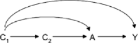
Figure 2: Definition 2 does not satisfy Property 2A or 2B.

We now show that it does not satisfy Properties 2A and 2B. Consider the causal diagram in Figure 2. Under Definition 2 both $C_{1}$ and $C_{2}$ block a backdoor path from $A$ to $Y$ and thus would qualify as confounders. However, for $C_{2}$ there is no set of pre-exposure covariates $X$ on the graph such that control for $C_{2}$ helps eliminate since if $X=C_{1}$, there is no bias without controlling for $C_{2}$; if $X=\varnothing$, there is bias even with controlling for $C_{2}$. Thus, Definition 2 does not satisfy Property 2A. We now show that it does not satisfy Property 2B. Suppose Figure 2 is a causal diagram for $(C_{1},C_{2},A,Y)$ where all variables are binary and suppose that $P(C_{1}=1)=1/2$, $P(C_{2}=1|c_{1})=1/5+3c_{1}/5$, $P(A=1|c_{1},c_{2})=1/10+3c_{1}/5+c_{2}/10$, $P(Y=1|a,c_{1},c_{2})=1/2+(1/2)(a-1/2)c_{1}$. One can then verify that $E(Y_{1})-E(Y_{0})=\sum_{c_{1},c_{2}}\{E(Y|A=1,c_{1},c_{2})-E(Y|A=0,c_{1},c_{2})\}\operatorname{pr}(c_{1},c_{2})=0.25=\sum_{c_{1}}\{E(Y|A=1,c_{1})-E(Y|A=0,c_{1})\}\operatorname{pr}(c_{1})$, that $E(Y|A=1)-E(Y|A=0)=0.266$ and that $\sum_{c_{2}}\{E(Y|A=1,c_{2})-E(Y|A=0,c_{2})\}\operatorname{pr}(c_{2})=0.269$. Under Definition 2, $C_{2}$ would be considered a confounder since $C_{2}$ blocks the backdoor path $A\leftarrow C_{2}\leftarrow C_{1}\rightarrow Y$. However, there is no set $X$ of pre-exposure covariates such that $|\sum_{x,c_{2}}\{E(Y|A=1,x,c_{2})-E(Y|A=0,x,\break c_{2})\}\operatorname{pr}(x,c_{2})-\{E(Y_{1})-E(Y_{0})\}|<|\sum_{x}\{E(Y|A=1,x)-E(Y|A=\break 0,x)\}\operatorname{pr}(x)-\{E(Y_{1})-E(Y_{0})\}|$. This is because if $X$ is taken as $C_{1}$, then the expressions on both sides of the inequality are equal to $0$ (controlling for $C_{2}$ in addition to $C_{1}$ does not reduce bias); if $X$ is taken as the empty set, we have $|\sum_{c_{2}}\{E(Y|A=1,c_{2})-E(Y|A=0,c_{2})\}\operatorname{pr}(c_{2})-\{E(Y_{1})-E(Y_{0})\}|=|0.269-0.250|=0.019>0.016=|0.266-0.250|=|\{E(Y|A=1)-E(Y|A=0)\}-\{E(Y_{1})-E(Y_{0})\}|$ and again controlling for $C_{2}$ does not reduce (but rather increases) bias. Definition 2 thus does not satisfy Property 2B. This completes the proof.

If we consider the causal diagram in Figure 2, then under Definition 2 both $C_{1}$ and $C_{2}$ block a backdoor path from $A$ to $Y$ and thus would qualify as confounders. However, for $C_{2}$ there is no set of pre-exposure covariates $X$ on the graph such that control for $C_{2}$ helps eliminate bias (Property 2A) since if $X=C_{1}$, there is no bias without controlling for $C_{2}$; if $X=\varnothing$, there is bias even with controlling for $C_{2}$. Likewise, examples can be constructed as in the proof above in which control for $C_{2}$ will only increase bias, that is, control for $C_{2}$ does not help reduce bias (Property 2B).

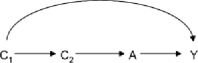
Figure 3: Definition 3 does not satisfy Property 1.

Under Definition 3, a confounder was defined as a member of every minimally sufficient adjustment set.

Proposition 3

Definition 3 does not satisfy Property 1. Definition 3 satisfies Property 2A.

Consider the causal diagram in Figure 3. Here, either $C_{1}$ or $C_{2}$ would constitute minimally sufficient adjustment sets and thus neither are a member of every minimally sufficient adjustment set and under Definition 3, neither would be confounders. If we control for nothing, there is still confounding for the effect of $A$ on $Y$ and, thus, for Figure 3, controlling for all confounders under Definition 3 would not suffice to control for confounding. Thus, Definition 3 does not satisfy Property 1. If $C$ is a member of every minimally sufficient adjustment set, then it is a member of a minimally sufficient adjustment set and from this it trivially follows that it satisfies the requirements in Property 2A. This completes the proof.

A variable $C$ that is a confounder under Definition 3 will in general satisfy Property 2B as well but may not always because there are cases in which there is confounding in the distribution of counterfactual outcomes conditional on $C$ and so that $C$ is a confounder under Definition 3 but with the average causal effect on the additive scale not confounded [Greenland, Robins and Pearl (1999)]. Intuitively, to see that Definition 3 does not satisfy Property 1, consider the causal diagram in Figure 3. Here, either $C_{1}$ or $C_{2}$ would constitute minimally sufficient adjustment sets and thus neither are a member of every minimally sufficient adjustment set. Under Definition 3, there would thus be no confounders for the effect of $A$ on $Y$; clearly, however, if we control for nothing, there is still confounding for the effect of $A$ on $Y$.

Under Definition 4, a confounder was defined as a member of some minimally sufficient adjustment set.

Proposition 4

For every causal diagram, Definition 4 satisfies Property 1. Definition 4 satisfies Property 2A.

We will show that Definition 4 satisfies Property 1. We first claim that any minimally sufficient adjustment set for $(A,Y)$ must lie in $G_{\mathrm{An}(A)\cup\mathrm{An}(Y)}$, the subgraph of $G$ that has only the nodes in $\operatorname{Nd}(A)$ or $\operatorname{An}(Y)$; see the Appendix. Assume this is not true, and pick some minimally sufficient set $S$ with elements outside $\operatorname{An}(A)\cup\operatorname{An}(Y)$. This means $S\cap(\operatorname{An}(A)\cup\operatorname{An}(Y))$ is not sufficient. Note that any ancestor of a node in the set $\operatorname{An}(A)\cup\operatorname{An}(Y)$ will also be in $\operatorname{An}(A)\cup\operatorname{An}(Y)$. From this it follows that any backdoor path from $A$ to $Y$ which has a node outside $\operatorname{An}(A)\cup\operatorname{An}(Y)$ will require a collider to get back into $\operatorname{An}(A)\cup\operatorname{An}(Y)$. However, those colliders must be open by elements in $S$. We have a contradiction. We have shown that any minimally sufficient adjustment set must be a subset of $\operatorname{An}(A)\cup\operatorname{An}(Y)$ and, thus, any variable that is a confounder under Definition 4 must be in $\operatorname{An}(A)\cup\operatorname{An}(Y)$.

Next we note that $\operatorname{Pa}(A)$ is a sufficient adjustment set for $(A,Y)$. Pick a minimal subset $\operatorname{Pa}^{+}$ of $\operatorname{Pa}(A)$ that is sufficient. Our claim is that every element $P$ in $\operatorname{Pa}(A)\setminus\operatorname{Pa}^{+}$ is such that $P$ is not connected to $Y$ in the graph $(G_{\mathrm{An}(A)\cup\mathrm{An}(Y)})_{\overline{a}}$ except by paths that are blocked conditional on $\operatorname{Pa}^{+}$. Assume this is not true, and fix a path $\omega$ from $P$ to $Y$ that is not blocked by $\operatorname{Pa}^{+}$ in $(G_{\mathrm{An}(A)\cup\mathrm{An}(Y)})_{\overline{a}}$. If this path has no colliders, then appending $\omega$ with the edge $P\rightarrow A$ produces a backdoor path from $A$ to $Y$ not blocked by $\operatorname{Pa}^{+}$, contradicting the earlier claim that $\operatorname{Pa}^{+}$ is a valid adjustment set.

If $\omega$ only contains colliders ancestral of $\operatorname{Pa}^{+}$, then either $\omega$ has a noncollider triple blocked by $\operatorname{Pa}^{+}$ (in which case we are done with that path) or $\omega$ appended with $P\rightarrow A$ produces a backdoor path open conditional on $\operatorname{Pa}^{+}$, which is a contradiction. If $\omega$ contains collider triples ancestral of $\operatorname{Pa}(A)\setminus\operatorname{Pa}^{+}$ (but not ancestral of $\operatorname{Pa}^{+}$), let $W$ be the central node of the last such collider triple on the path from $P$ to $Y$. Let $P^{\prime}$ be a member of $\operatorname{Pa}(A)\setminus\operatorname{Pa}^{+}$ of which $W$ is an ancestor. Consider instead of $\omega$ a new path: $A\leftarrow P^{\prime}\leftarrow\cdots\leftarrow W$ appended with the subpath of $\omega$ that begins with the node on $\omega$ after $W$ and ends with $Y$. This path either has a noncollider triple blocked by $\operatorname{Pa}^{+}$ (in which case so does $\omega$ and we are done with $\omega$) or it is open conditional on $\operatorname{Pa}^{+}$, in which case we have a contradiction, or it contains collider triples ancestral of $Y$ not through $\operatorname{Pa}(A)$. In the last case, let $Z$ be the central node of the first such collider triple on the currently considered path from $A$ to $Y$. Consider instead a new path which appends a subpath of the currently considered path extending from $A$ to $Z$, and the segment $Z\rightarrow\cdots\rightarrow Y$. This path has no blocked colliders by construction, and thus must either have a noncollider triple blocked by $\operatorname{Pa}^{+}$ (in which case so does $\omega$ and we are done with $\omega$) or it is open conditional on $\operatorname{Pa}^{+}$, in which case we have a contradiction.

Our final claim is that any superset $S$ of $\operatorname{Pa}^{+}$ in $\operatorname{Nd}(A)\cap(\operatorname{An}(A)\cup\operatorname{An}(Y))$ is a valid adjustment set for $(A,Y)$. Assume this were not so and fix an open backdoor path $\rho$ from $A$ to $Y$ given $S$. The first node on $\rho$ after $A$ must lie either in $\operatorname{Pa}^{+}$ or in $\operatorname{Pa}(A)\setminus\operatorname{Pa}^{+}$. In the first case, the path is blocked. In the second case, we have shown above that every path from $\operatorname{Pa}(A)\setminus\operatorname{Pa}^{+}$ to $Y$ in $(G_{\mathrm{An}(A)\cup\mathrm{An}(Y)})_{\overline{a}}$ is blocked by $\operatorname{Pa}^{+}$ and, thus, the path must be blocked in the second case as well. There thus cannot be an open backdoor path from $A$ to $Y$ given $S$ and we have a contradiction. We have that $\operatorname{Pa}^{+}$ is a sufficient adjustment set; any variable that is a confounder under Definition 4 will be a member of $\operatorname{Nd}(A)\cap(\operatorname{An}(A)\cup\operatorname{An}(Y))$ and, thus, we have that the set of variables that are confounders under Definition 4 will be a sufficient adjustment set. Definition 4 thus satisfies Property 1. Definition 4 satisfies Property 2A trivially. This completes the proof.

A variable that is a confounder under Definition 4 will in general satisfy Property 2B as well but may not always because, as before, there may be confounding in distribution without the average causal effect on the additive scale being confounded. Definition 4 thus satisfies Property 2A, generally Property 2B, and, as shown in the proof above, also satisfies Property 1 for all causal diagrams. That Definition 4 satisfies Property 1 can be restated as the proposition that the union of all minimally sufficient adjustment sets is itself a sufficient adjustment set. Definition 4 thus satisfies the properties which arguably ought to be required for a reasonable definition of a “confounder.”

Under Definition 5, a confounder was essentially defined as a pre-exposure covariate, the control for which helped reduce bias.

Proposition 5

Definition 5 does not satisfy Property 1. Definition 5 satisfies Property 2B but not 2A.

Suppose that $Y_{a}\perp\!\!\!\perp A|C$, that $(C,A,Y)$ are all binary and that $P(C=1)=1/2$, $P(A=1|c)=1/4+c/2$, $P(Y=1|a,c)=4/10-4c/10-3a/10+8ac/10$. One can then verify that $E(Y_{1})=\sum_{c}E(Y|A=1,c)\operatorname{pr}(c)=3/10$, $E(Y|A=1)=4/10$, $E(Y_{0})=\sum_{c}E(Y|A=0,c)\operatorname{pr}(c)=2/10$, $E(Y|A=0)=3/10$. Thus, $|\sum_{c}\{E(Y|A=1,c)-E(Y|A=0,c)\}\operatorname{pr}(c)-\break\{E(Y_{1})-E(Y_{0})\}|=0=|\{E(Y|A=1)-E(Y|A=0)-\{E(Y_{1})-E(Y_{0})\}|$ and so under Definition 5, $C$ would not be a confounder. The set of variables defined as confounders under Definition 5 would thus be empty. However, it is not the case that adjustment for the empty set suffices to control for confounding since, for example, $E(Y_{1})=3/10\neq 4/10=E(Y|A=1)$. Thus, Definition 5 does not satisfy Property 1. We now show that Definition 5 does not satisfy Property 2A. Consider the causal diagram in Figure 4. Although control for $C_{2}$ might reduce bias compared to an unadjusted estimate and thus satisfy Definition 5 with $X=\varnothing$, there is no $X$ such that the effect of $A$ on $Y$ is unconfounded conditional on $(X,C_{2})$ but not on $X$ alone. Thus, Definition 5 does not satisfy Property 2A. Definition 5 satisfies Property 2B trivially. This completes the proof.

Definition 5 does not satisfy Property 1 because an unadjusted estimate of the causal risk difference may be correct, even in the presence of confounding, because the bias due to confounding for $E(Y_{1})$ may cancel that for $E(Y_{0})$; said another way, there may be confounding in the distribution of counterfactual outcomes without their being confounding in a particular measure. That Definition 5 satisfies Property 2B is essentially embedded in Definition 5 itself. Intuitively, to see that Definition 5 does not satisfy Property 2A, consider the causal diagram in Figure 4. Although control for $C_{2}$ might reduce bias compared to an unadjusted estimate and thus satisfy Definition 5 with $X=\varnothing$, there would be no $X$ such that the effect of $A$ on $Y$ is unconfounded conditional on $(X,C_{2})$ but not on $X$ alone.

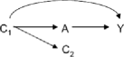
Figure 4: Definition 5 does not satisfy Property 2A.

Under Definition 6, a confounder was defined as a pre-exposure covariate, the control for which in some context changed the effect estimate.

Proposition 6

Definition 6 does not satisfy Property 1. Definition 6 does not satisfy Properties 2A or 2B.

In the first example in the proof of Proposition 5, the set of confounders under Definition 6 would be empty because with $X$ empty we have $\sum_{x,c}\{E(Y|A=1,x,c)-E(Y|A=0,x,c)\}\operatorname{pr}(x,c)=0=\sum_{x}\{E(Y|A=1,x)-E(Y|A=0,x)\}\operatorname{pr}(x)$. However, the effect of $A$ on $Y$ is not unconfounded conditional on the empty set. Thus, Definition 6 does not satisfy Property 1.

We now show Definition 6 does not satisfy Properties 2A or 2B. Consider the causal diagram in Figure 1. If we let $X$ denote the empty set, then $C_{3}$ will satisfy Definition 6 and so would be a confounder under Definition 6. However, if we consider Properties 2A and 2B, there is no set of pre-exposure covariates $X$ on the graph such that control for $C_{3}$ helps eliminate or reduce bias. To see this, note that if $X$ includes $C_{1}$ or $C_{2}$, then the effect estimate is unbiased irrespective of whether adjustment is made for $C_{3}$. If $X$ includes neither $C_{1}$ nor $C_{2}$, then the estimand without adjustment for $C_{3}$ is unbiased whereas the estimand adjusted for $C_{3}$ is not. Therefore, Definition 1 does not satisfy Properties 2A and 2B. This completes the proof.

As with Definition 5, Definition 6 does not satisfy Property 1 because of the possibility of cancellations: there may be confounding in the distribution of counterfactual outcomes without their being confounding in a particular measure. Definition 6 also fails to satisfy Properties 2A or 2B. It fails because of the possibility of “M-bias” or “collider-stratification” structures as in Figure 1 [Greenland (2003), Hernán et al. (2002)]. Controlling for a variable such as $C_{3}$ may change the estimate, but it may be that it is the estimate without control for that variable (e.g., $C_{3}$ in Figure 1) that is unbiased. Also, as noted above, the collapsibility-based definitions fail for odds ratio and hazard ratio measures for others reasons, namely, because marginal and conditional measures are not comparable even in the absence of confounding. See Greenland, Robins and Pearl (1999), Geng et al. (2001) and Geng and Li (2002) for further discussion of the relationship between, and general nonequivalence of, confounding and collapsibility.

Candidate definitions for a confounder might thus include Definition 4 and, if the issue of scale dependence is set aside, Definition 5. Note, however, that a variable that satisfies Definition 5 but not Definition 4 will never help to eliminate confounding bias, only to reduce such bias. Such a variable reduces bias essentially by serving as a proxy for a variable that does satisfy Definition 4. We therefore propose that a confounder be defined as in Definition 4, “a pre-exposure covariate that is a member of some minimally sufficient adjustment set” and that any variable that satisfies Definition 5 but not Definition 4 be referred to as a “surrogate confounder.” The terminology of a “surrogate confounder” or “proxy confounder” appears elsewhere [Greenland and Morgenstern (2001), Hernán (2008)]; here we have provided a formal criterion for such a “surrogate confounder.” See Greenland and Pearl (2011) and Ogburn and VanderWeele (2012) for properties of such surrogate confounders.

Interestingly, Definition 4 is closely related to definitions concerning confounders proposed by Robins and Morgernstern (1987), though their definitions were not universally adopted by the epidemiologic community over the ensuing 25 years. Robins and Morgenstern (1987) were not principally concerned with how the word “confounder” is employed in practice when used in an unqualified sense, but rather with whether a particular variable would still, in some sense, be a confounder if data were also available on other variables. As noted above, Robins and Morgenstern [(1987), Section 2H] say that $C$ is a confounder conditional on $F$ if causal effects are computable given data on $C$ and $F$, but not on $F$ alone. In the framework of Robins and Morgenstern, if one were to take as the (unconditional) definition of a confounder that “there exists some set $F$ such that $C$ is a confounder conditional on $F$ [in the sense of Robins and Morgenstern (1987), Section 2H],” then this would coincide with Definition 4. Note that Robins and Morgenstern, in their definitions, in some sense go further than Definition 4 in having the investigator explicitly specify the other variables $F$ for which control might be made. This would indeed be useful in practice, though current use of language has not generally adopted this convention. It might in the future be helpful to distinguish between the unqualified use of the word “confounder” as defined in Definition 4, and “confounder in the context of having data also on $F$” as in Robins and Morgenstern (1987). The former is arguably how the word “confounder” is often used in practice; the latter would be useful in making decisions about data collection and confounder control.

6 Some extensions, implications and further results

In the discussion above we have considered whether a covariate is a “confounder” in an unconditional sense. However, we might also speak about whether a variable $C$ is a confounder for the effect of $A$ on $Y$ conditional on some set of covariates $L$ which an investigator is going to condition on irrespective of whether control is made for $C$. Definition 4 above, the definition for an “unconditional confounder” could be restated as follows: a pre-exposure covariate $C$ is a confounder for the effect of $A$ on $Y$ if there exists a set of pre-exposure covariates $X$ such that $Y_{a}\perp\!\!\!\perp A|(X,C)$ but there is no proper subset $T$ of $(X,C)$ such that $Y_{a}\perp\!\!\!\perp A|T$. The conditional analogue would then be as follows: we say that a pre-exposure covariate $C$ is a confounder for the effect of $A$ on $Y$ conditional on $L$ if there exists a set of pre-exposure covariates $X$ such that $Y_{a}\perp\!\!\!\perp A|(X,L,C)$ but there is no proper subset $T$ of $(X,C)$ such that $Y_{a}\perp\!\!\!\perp A|(T,L)$. Consider again the causal diagram in Figure 3. Here, $C_{2}$ would be a confounder under Definition 4. However, $C_{2}$ is not a confounder for the effect of $A$ on $Y$ conditional on $L=C_{1}$. Consider once more the causal diagram in Figure 1. Here, neither $C_{1}$ nor $C_{2}$ would be a confounder under Definition 4. However, conditional on $L=C_{3}$, both $C_{1}$ and $C_{2}$ would be confounders.

An analogue of Definition 4 could also be given for a particular causal parameter of interest rather than for the condition of nonconfounding in distribution $Y_{a}\perp\!\!\!\perp A|S$. For example, $C$ could be defined to be a confounder for a particular causal parameter (e.g., the causal risk difference or causal risk ratio) if there exists a set of pre-exposure covariates $X$ such the parameter is identified by adjusting for $(X,C)$ and if for no proper subset, $T$ of $(X,C)$ is the parameter identified by adjusting for $T$ [cf. Robins and Morgenstern (1987)]. However, when we restrict attention to particular parameters we reintroduce some of the complications with cancellations that were noted above. For example, due to cancellations, a variable $C$ may be a confounder for the causal risk difference but not for the causal risk ratio [cf. VanderWeele (2012)].

We have restricted our attention in this paper thus far to pre-exposure covariates as potential confounders. We have done so in order to correspond as closely as possible to the discussion in the epidemiologic and potential outcomes literatures. However, within the context of causal diagrams, a somewhat broader range of variables could be considered as “confounders” in that all of the discussion above is applicable if we consider all nondescendents of $A$ as potential confounders rather than simply considering pre-exposure covariates.

Throughout the paper we have given all definitions with respect to a particular underlying causal diagram. However, for a given exposure $A$ and a given outcome $Y$, there will be multiple causal diagrams that correctly represent the causal structure relating these variables to one another and to covariates. One diagram may be an elaboration of another and contain variables that the other does not. It is straightforward to verify that if a variable $C$ is classified as a confounder under Definitions 1, 2, 4, 5 or 6, then $C$ will also be a confounder under each of those definitions respectively on any expanded causal diagram with additional variables. In the case of Definition 1, this is because associations that hold conditional on covariates $X$ for one diagram will clearly also hold for the other. In the case of Definition 2, if $C$ blocks a backdoor path on one causal diagram, it will block a backdoor path on any larger diagram that also correctly describes the causal structure. In the case of Definition 4, if there is some minimally sufficient adjustment set $S$ of which $C$ is a member, then that set will also be minimally sufficient on any larger diagram that also correctly describes the causal structure. In the case of Definitions 5 and 6, if the inequalities in these definitions hold for some covariate set $X$ for one diagram, they will clearly also hold for the other. Only Definition 3 does not share this property. To see this, consider Figure 3; if in Figure 3, we collapsed over $C_{2}$ so that the causal diagram involved only $C_{1}$, $A$ and $Y$, then $C_{1}$ would be a member of every minimally sufficient adjustment set for this diagram and thus a confounder under Definition 3. However, as we saw above, $C_{1}$ is not a confounder under Definition 3 for Figure 3 itself which includes the extra variable $C_{2}$. This failure is a serious problem with Definition 3, but, as we also saw above, Definition 3 suffers from other limitations as well.

Several fairly trivial implications follow from Definition 4 and may be worth noting for the sake of completeness. First, if a causal diagram had a variable $C$ with an arrow to $\log(C)$ (or vice versa) and if $C$ were a member of a minimally sufficient adjustment set, then, under Definition 4, both $C$ and $\log(C)$ would be considered “confounders,” though $\log(C)$ would not be a confounder conditional on $C$, and likewise $C$ would not be a confounder conditional on $\log(C)$. We believe that this is in accord with epidemiologic usage, though it would be peculiar to consider both $C$ and $\log(C)$ simultaneously, just as it would be peculiar to include both $C$ and $\log(C)$ on a causal diagram. Second, if a variable $C$ is measured with error, taking value $C^{\ast}$, and if the measurement error term $\varepsilon=C^{\ast}-C$ were also represented on the causal diagram, then, if $C$ were a confounder under Definition 4, $C^{\ast}$ and $\varepsilon$ would also both be confounders under Definition 4. We believe this is also in accord with standard epidemiologic usage of “confounder,” though we would in practice rarely refer to $\varepsilon$ as a “confounder” since we rarely have access to $\varepsilon$. Once again, however, neither $C^{\ast}$ nor $\varepsilon$ would be confounders conditional on $C$. Finally, suppose $C_{1}$ were height in meters and $C_{2}$ were weight in kilograms and that $C_{1}$ and $C_{2}$ together sufficed to control for confounding but neither alone did; let $C_{3}=C_{1}/C_{1}^{2}$ be body mass index (BMI) and suppose that controlling for $C_{3}$ alone sufficed to control for confounding. Then under Definition 4, $C_{1}$, $C_{2}$ and $C_{3}$ would each be confounders, though $C_{3}$ would not be a confounder conditional on $(C_{1},C_{2})$ and likewise neither $C_{1}$ nor $C_{2}$ would be a confounder conditional on $C_{3}$. Once again, we believe this is in accord with traditional epidemiologic usage of “confounder.”

Several implications hold between the different definitions of a confounder as stated in the following result.

Proposition 7

On a causal diagram, if a variable is a confounder under Definition 3, then it is a confounder under Definitions 4, 2 and 1; if under Definition 4, then under Definitions 2 and 1; if under Definition 5, then under Definitions 6 and 1; if under Definition 6, then under Definition 1. No other implications hold without further assumptions.

On a causal diagram, if a variable is a member of every minimally sufficient adjustment set, it must be a member of a minimally sufficient adjustment set (the existence of a minimally sufficient adjustment set is guaranteed by the variables lying on a causal diagram). Thus, if a variable is a confounder under Definition 3, then it is a confounder under Definition 4. Suppose a variable $C$ satisfies Definition 4, that is, is a member of some minimally sufficient adjustment set $(X,C)$, but that it does not satisfy Definition 2, that is, it is not on a backdoor path from $A$ to $Y$. By Theorem 5 of Shpitser, VanderWeele and Robins (2010), $(X,C)$ blocks all backdoor paths from $A$ to $Y$. If $C$ does not lie on a backdoor path from $A$ to $Y$, then $X$ alone would block all backdoor paths from $A$ to $Y$, which would contradict that $(X,C)$ is a minimally sufficient adjustment set. Thus, if $C$ is a confounder under Definition 4, it is a confounder under Definition 2. That $C$ being a confounder under Definition 4 implies $C$ is a confounder under Definition 1 follows from the contrapositive of Corollary 4.1 of Robins (1997). If $C$ is a confounder under Definition 5, it must be a confounder under Definition 6 because the only way $C$ can be a confounder under Definition 5 is if $\sum_{x,c}\{E(Y|A=1,x,c)-E(Y|A=0,x,c)\}\operatorname{pr}(x,c)$ and $\sum_{x}\{E(Y|A=1,x)-E(Y|A=0,x)\}\operatorname{pr}(x)$ are not equal. If $C$ is not a confounder under Definition 1, then for every $X$, $C$ is independent of $Y$ conditional on $(A,X)$ or of $A$ conditional on $X$ and from this it easily follows that $\sum_{x,c}\{E(Y|A=1,x,c)-E(Y|A=0,x,c)\}\operatorname{pr}(x,c)=\sum_{x}\{E(Y|A=1,x)-E(Y|A=0,x)\}\operatorname{pr}(x)$ and thus that $C$ is not a confounder under Definition 6. Thus, if $C$ is a confounder under Definition 6, it must be a confounder under Definition 1.

We now argue that without further assumptions no other implications between the definitions hold. The variable $C_{2}$ in Figure 4 could satisfy Definition 1 but does not satisfy Definition 2, so Definition 1 does not imply Definition 2. The variable $C_{3}$ in Figure 1 could satisfy Definition 1, but does not satisfy Definitions 3, 4 or 5; thus, Definition 1 does not imply Definitions 3, 4 or 5. If $C$ is a confounder under Definition 1, in general it will be under Definition 6 as well, but it may not because of cancellations due to scale-dependence.

If $C$ satisfies the conditions for Definition 2 (i.e., lies on a backdoor path from $A$ to $Y$), it will generally do so for Definitions 1 and 6 but may fail to do so because of failure or faithfulness or cancellations due to scale-dependence. In the example given concerning Property 2B in Proposition 2, the variable $C_{2}$ in Figure 2 satisfied Definition 2 but does not satisfy Definitions 3, 4 or 5; thus, Definition 2 does not imply Definitions 3, 4 or 5.

It was shown above that if $C$ satisfies the conditions for Definition 3, it will satisfy the conditions for Definitions 4, 2 and 1. If $C$ satisfies the conditions for Definition 3, it will generally satisfy the conditions for Definitions 5 and 6, but it may not do so due to scale-dependence.

It was shown above that if $C$ satisfies the conditions for Definition 4, it will satisfy the conditions for Definitions 2 and 1. In Figure 3, $C_{2}$ satisfies the conditions for Definition 4 but not Definition 3, therefore, Definition 4 does not imply Definition 3. If $C$ satisfies the conditions for Definition 4, it will generally satisfy the conditions for Definitions 5 and 6, but it may not do so due to scale-dependence.

It was shown above that if $C$ satisfies the conditions for Definition 5, it will satisfy the conditions for Definitions 6 and 1. In the example given concerning Property 2B in Proposition 5, the variable $C_{2}$ in Figure 4 satisfied Definition 5 but does not satisfy Definitions 2, 3 or 4; thus, Definition 5 does not imply Definitions 2, 3 or 4.

It was shown above that if $C$ satisfies the conditions for Definition 6, it will satisfy the conditions for Definition 1. The variable $C_{2}$ in Figure 4 could satisfy Definition 6 but does not satisfy Definition 2, so Definition 6 does not imply Definition 2. The variable $C_{3}$ in Figure 1 could satisfy Definition 6, but does not satisfy Definitions 3, 4 or 5; thus, Definition 6 does not imply Definitions 3, 4 or 5.

Figure 5: Logical relationships that hold among definitions. Dashed arrows indicate implications that will generally hold but may fail due to scale dependence of definitions.

The implications between the definitions are plotted in Figure 5. Those implications that will generally hold but may not hold because of cancellations due to scale-dependence are indicated with dashed arrows.

The properties themselves that we have been considering also bear certain relations to one another insofar as it is not difficult to show that if Property 2A is itself taken as the definition of a confounder, then, on causal diagrams, this definition of a confounder also satisfies Property 1. This is because if $S$ denotes the set of all nodes $C$ which obey Property 2A and if $S$ is not a sufficient adjustment set (so there is open backdoor path $\pi$ from $A$ to $Y$), then if we let $W$ be all nondescendants of $A$ other than $A$ and noncolliders nodes on $\pi$, if we choose a node $K$ on $\pi$ that does not contain descendants of $A,$ then it is the case that $K$ satisfies Property 2A, and is not a part of $S$, which would be a contradiction.

Although it is the case that if Property 2A is itself taken as the definition of a confounder then this definition also satisfies Property 1 on causal diagrams, this does not hold generally within a counterfactual framework. Note also that, even on causal diagrams, it is not the case that Property 2A implies Property 1; a counterexample to this was given in Proposition 3 for Definition 3 which satisfies Property 2A but not Property 1. Rather, if Property 2A is itself taken as the definition of a confounder, then, on causal diagrams, this definition would satisfy Property 1 as well. This raises the question as to whether Property 2A itself could be taken as the definition of a confounder, as such a definition would satisfy Property 2A (by definition) and Property 1 on causal diagrams. Although such a definition would satisfy Properties 1 and 2A on causal diagrams, it would also follow from this definition that $C_{1}$ is a confounder for the effect of $A$ on $Y$ in Figure 1, even though the effect $A$ on $Y$ is unconfounded without controlling for any covariates. This is because if Property 2A is taken as the definition of a confounder, then $C_{1}$ satisfies Property 2A with $X$ taken as $C_{3}$. In general, however, if the effect $A$ on $Y$ is unconfounded without controlling for any covariates, we would probably simply say that there are no confounders for the unconditional effect of $A$ on $Y$.

7 Concluding remarks

The causal inference literature has provided a formal definition of confounding with reference to distributions of counterfactual outcomes. The literature now rightly emphasizes the concept of confounding control over that of a “confounder.” Nonetheless, the word “confounder” is often still used among applied researchers and in this paper we have shown that at least one formal counterfactual-based definition coheres with the way in which the word is generally used. We have considered a number of candidate proposals often arising from more informal statements made in the literature. We have considered whether each of these definitions satisfies two properties, namely, (i) that on any causal diagram, control for all confounders so defined will control for confounding and (ii) any variable qualifying as a confounder under this criterion will in some context remove confounding. Only one of the definitions considered here satisfied both of these two properties. We thus proposed that a pre-exposure covariate $C$ be considered a confounder for the effect of $A$ on $Y$ if there exists a set of covariates $X$ such that the effect of the exposure on the outcome is unconfounded conditional on $(X,C)$ but for no proper subset of $(X,C)$ is the effect of the exposure on the outcome unconfounded given the subset. Equivalently, a confounder is a “member of a minimally sufficient adjustment set.” This is closely related to the definitions concerning confounders given in Robins and Morgenstern (1987), though Robins and Morgenstern suggest specifying the other variables for which control might be made as well. We have further provided a conditional analogue of the proposed definition of a confounder; and we have proposed that a variable that helps reduce bias but not eliminate bias be referred to as a “surrogate confounder.” The definition of a “confounder” above is given rigorously in terms of counterfactuals and, we believe, is also in accord with the intuitive properties of a “confounder” implicitly presupposed by practicing statisticians and epidemiologists. From a more theoretical perspective, Definition 4, unlike the other definitions, gives rise to elegant and useful results which itself lends further support for its being taken as the definition of a confounder.

Appendix

Review of causal diagrams

A directed graph consists of a set of nodes and directed edges among nodes. A path is a sequence of distinct nodes connected by edges regardless of arrowhead direction; a directed path is a path which follows the edges in the direction indicated by the graph’s arrows. A directed graph is acyclic if there is no node with a sequence of directed edges back to itself. The nodes with directed edges into a node $A$ are said to be the parents of $A$; the nodes into which there are directed edges from $A$ are said to be the children of $A$. We say that node $A$ is an ancestor of node $B$ if there is a directed path from $A$ to $B$; if $A$ is an ancestor of $B$, then $B$ is said to be a descendant of $A$. If $X$ denotes a set of nodes, then $\operatorname{An}(X)$ will denote the ancestors of $X$ and $\operatorname{Nd}(X)$ will denote the set of nondescendants of $X$. For a given graph $G$, and a set of nodes $S$, the graph $G_{S}$ denotes a subgraph of $G$ containing only vertices of $G$ in $S$ and only edges of $G$ between vertices in $S$. On the other hand, the graph $G_{\overline{S}}$ denotes the graph obtained from $G$ by removing all edges with arrowheads pointing to $S$. A node is said to be a collider for a particular path if it is such that both the preceding and subsequent nodes on the path have directed edges going into that node. A path between two nodes, $A$ and $B$, is said to be blocked given some set of nodes $C$ if either there is a variable in $C$ on the path that is not a collider for the path or if there is a collider on the path such that neither the collider itself nor any of its descendants are in $C$. For disjoint sets of nodes $A$, $B$ and $C$, we say that $A$ and $B$ are d-separated given $C$ if every path from any node in $A$ to any node in $B$ is blocked given $C$. Directed acyclic graphs are sometimes used as statistical models to encode independence relationships among variables represented by the nodes on the graph [Lauritzen (1996)]. The variables corresponding to the nodes on a graph are said to satisfy the global Markov property for the directed acyclic graph (or to have a distribution compatible with the graph) if for any disjoint sets of nodes $A,B,C$ we have that $A\perp\!\!\!\perp B|C$ whenever $A$ and $B$ are d-separated given $C$. The distribution of some set of variables $V$ on the graph is said to be faithful to the graph if for all disjoint sets $A,B,C$ of $V$ we have that $A\perp\!\!\!\perp B|C$ only when $A$ and $B$ are d-separated given $C$.

Directed acyclic graphs can be interpreted as representing causal relationships. Pearl (1995) defined a causal directed acyclic graph as a directed acyclic graph with nodes $(X_{1},\ldots,X_{n})$ corresponding to variables such that each variable $X_{i}$ is given by its nonparametric structural equation $X_{i}=f_{i}(pa_{i},\varepsilon_{i})$, where $pa_{i}$ are the parents of $X_{i}$ on the graph and the $\varepsilon_{i}$ are mutually independent. For a causal diagram, the nonparametric structural equations encode counterfactual relationships among the variables represented on the graph. The equations themselves represent one-step ahead counterfactuals with other counterfactuals given by recursive substitution [see Pearl (2009) for further discussion]. A causal directed acyclic graph defined by nonparametric structural equations satisfies the global Markov property as stated above [Pearl (2009)]. The requirement that the $\varepsilon_{i}$ be mutually independent is essentially a requirement that there is no variable absent from the graph which, if included on the graph, would be a parent of two or more variables [Pearl (1995, 2009)]. Throughout we assume the exposure $A$ consists of a single node. A backdoor path from $A$ to $Y$ is a path to $Y$ which begins with an edge into $A$. A set of variables $X$ is said to satisfy the backdoor path criterion with respect to $(A,Y)$ if no variable in $X$ is a descendant of $A$ and if $X$ blocks all backdoor paths from $A$ to $Y$. Pearl (1995) showed that if $X$ satisfies the backdoor path criterion with respect to $(A,Y)$, then the effect of $A$ on $Y$ is unconfounded given $X$, that is, $Y_{a}\perp\!\!\!\perp A|X$.

Empirical testing for confounders and confounding

The absence of confounding conditional on a set of covariates $S$, that is, $Y_{a}\perp\!\!\!\perp A|S$, is not a property that can be tested empirically with data. One must rely on subject matter knowledge, which may sometimes take the form of a causal diagram. Nonetheless, a few things can be said about empirical testing concerning confounding and confounders. For the sake of completeness, we will consider each of Definitions 1–6. It is possible to verify empirically whether a variable is a confounder under Definition 1 since the definition refers to observed associations; however, it is not possible, without further knowledge, to empirically verify that a variable does not satisfy Definition 1 because a variable may satisfy Definition 1 for some $X$ that involves an unmeasured variable $U$. One would have to know that data were available for all variables on a causal diagram to empirically verify that a variable was a nonconfounder under Definition 1. Because of this, even though Definition 1 satisfies Property 1 under faithfulness, this cannot be used as an empirical test for confounding since (i) we cannot empirically verify that a variable is a nonconfounder under Definition 1 and (ii) we cannot empirically verify whether faithfulness holds.

Without further assumptions, we cannot empirically verify that a variable is a confounder or a nonconfounder under Definition 2 because Definition 2 makes reference to backdoor paths. Whether a variable lies on a backdoor path cannot be tested empirically without further assumptions; one would have to know the structure of the underlying causal diagram. Likewise, for Definitions 3 and 4, one would need to know all minimally sufficient adjustment sets, which itself would require checking the “no confounding” condition $Y_{a}\perp\!\!\!\perp A|S$, which is, as noted above, not empirically testable; though see below for some qualifications. For Definition 5, we could empirically reject the inequality in Definition 5 for observed $X$ if $\sum_{x,c}\{E(Y|A=1,x,c)-E(Y|A=0,x,c)\}\operatorname{pr}(x,c)=\sum_{x}\{E(Y|A=1,x)-E(Y|A=0,x)\}\operatorname{pr}(x)$. However, we cannot empirically reject the inequality in Definition 5 for unobserved $X$ and we, moreover, cannot empirically verify the inequality in Definition 5 because $E(Y_{1})-E(Y_{0})$ will not in general be empirically identified if there are unobserved variables. We can verify empirically whether a variable is a confounder under Definition 6 since the definition refers to only observed variables; however, it is not possible, without further knowledge, to empirically verify that a variable does not satisfy Definition 6 because a variable may satisfy Definition 6 for some $X$ that involves an unmeasured variable $U$. One would have to know that data were available for all variables on a causal diagram to empirically verify that a variable was a nonconfounder under Definition 6. Because of this we cannot empirically verify that a variable is a nonconfounder under Definition 6.

Determining whether a variable is a confounder requires making untestable assumptions. The only real progress that can be made with empirical testing for confounders is by making other untestable assumptions that logically imply a test for assumptions we care about. For example, suppose we assume we have some set $S$ that we are sure constitutes a sufficient adjustment set. In this case, we can sometimes remove variables as unnecessary for confounding control. In particular, Robins (1997) showed that if we knew that for covariate sets $S_{1}$ and $S_{2}$ we had that $Y_{a}\perp\!\!\!\perp A|(S_{1},S_{2})$, then we would also have that $Y_{a}\perp\!\!\!\perp A|S_{1}$ if $S_{2}$ can be decomposed into two disjoint subsets $T_{1}$ and $T_{2}$ such that $A\perp\!\!\!\perp T_{1}|S_{1}$ and $Y\perp\!\!\!\perp T_{2}|A,S_{1},T_{1}$. Both of these latter conditions are empirically testable. Geng et al. (2001) provide some analogous results for the effect of exposure on the exposed. VanderWeele and Shpitser (2011) note that if for covariate set $S$ we have that $Y_{a}\perp\!\!\!\perp A|S$, then if a backward selection procedure is applied to $S$ such that variables are iteratively discarded that are independent of $Y$ conditional on both exposure $A$ and the members of $S$ that have not yet been discarded, then the resulting set of covariates will suffice for confounding control. They also show that under an additional assumption of faithfulness, if, for covariate set $S$, we have that $Y_{a}\perp\!\!\!\perp A|S$, then if a forward selection procedure is applied to $S$ such that, starting with the empty set, variables are iteratively added which are associated with $Y$ conditional on both exposure $A$ and the variables that have already been added, then the resulting set of covariates will suffice for confounding control. Note, however, all of these results require knowledge that for some set $S$, $Y_{a}\perp\!\!\!\perp A|S$, which is not itself empirically testable without experimental interventions.

References

- Barnow, Cain and Goldberger (1980) {bincollection}[auto:STB—2012/11/05—08:49:14] \bauthor\bsnmBarnow, \bfnmB. S.\binitsB. S., \bauthor\bsnmCain, \bfnmG. G.\binitsG. G. and \bauthor\bsnmGoldberger, \bfnmA. S.\binitsA. S. (\byear1980). \btitleIssues in the analysis of selectivity bias. In \bbooktitleEvaluation Studies (\beditor\bfnmE.\binitsE. \bsnmStromsdorfer and \beditor\bfnmG.\binitsG. \bsnmFarkas, eds.) \bvolume5. \bpublisherSage, \blocationSan Francisco. \bptokimsref \endbibitem
- Breslow and Day (1980) {bbook}[auto:STB—2012/11/05—08:49:14] \bauthor\bsnmBreslow, \bfnmN. E.\binitsN. E. and \bauthor\bsnmDay, \bfnmN. E.\binitsN. E. (\byear1980). \btitleStatistical Methods in Cancer Research, Vol. 1: The Analysis of Case–Control Studies. \bpublisherInternational Agency for Research on Cancer, \blocationLyon, France. \bptokimsref \endbibitem
- Cox (1958) {bbook}[mr] \bauthor\bsnmCox, \bfnmD. R.\binitsD. R. (\byear1958). \btitlePlanning of Experiments. \bpublisherWiley, \blocationNew York. \bidmr=0095561 \bptokimsref \endbibitem
- Dawid (2002) {barticle}[auto:STB—2012/11/05—08:49:14] \bauthor\bsnmDawid, \bfnmA. P.\binitsA. P. (\byear2002). \btitleInfluence diagrams for causal modeling and inference. \bjournalInt. Statist. Rev. \bvolume70 \bpages161–189. \bptokimsref \endbibitem
- Geng, Guo and Fung (2002) {barticle}[mr] \bauthor\bsnmGeng, \bfnmZhi\binitsZ., \bauthor\bsnmGuo, \bfnmJianhua\binitsJ. and \bauthor\bsnmFung, \bfnmWing-Kam\binitsW.-K. (\byear2002). \btitleCriteria for confounders in epidemiological studies. \bjournalJ. R. Stat. Soc. Ser. B Stat. Methodol. \bvolume64 \bpages3–15. \biddoi=10.1111/1467-9868.00321, issn=1369-7412, mr=1881841 \bptokimsref \endbibitem
- Geng and Li (2002) {barticle}[mr] \bauthor\bsnmGeng, \bfnmZhi\binitsZ. and \bauthor\bsnmLi, \bfnmGuangwei\binitsG. (\byear2002). \btitleConditions for non-confounding and collapsibility without knowledge of completely constructed causal diagrams. \bjournalScand. J. Stat. \bvolume29 \bpages169–181. \biddoi=10.1111/1467-9469.00087, issn=0303-6898, mr=1894389 \bptokimsref \endbibitem
- Geng et al. (2001) {barticle}[mr] \bauthor\bsnmGeng, \bfnmZhi\binitsZ., \bauthor\bsnmGuo, \bfnmJianhua\binitsJ., \bauthor\bsnmLau, \bfnmTai Shing\binitsT. S. and \bauthor\bsnmFung, \bfnmWing-Kam\binitsW.-K. (\byear2001). \btitleConfounding, homogeneity and collapsibility for causal effects in epidemiologic studies. \bjournalStatist. Sinica \bvolume11 \bpages63–75. \bidissn=1017-0405, mr=1820001 \bptokimsref \endbibitem
- Glymour and Greenland (2008) {bincollection}[auto:STB—2012/11/05—08:49:14] \bauthor\bsnmGlymour, \bfnmM. M.\binitsM. M. and \bauthor\bsnmGreenland, \bfnmS.\binitsS. (\byear2008). \btitleCausal diagrams. In \bbooktitleModern Epidemiology, \bedition3rd ed. (\beditor\bfnmK. J.\binitsK. J. \bsnmRothman, \beditor\bfnmS.\binitsS. \bsnmGreenland and \beditor\bfnmT. L.\binitsT. L. \bsnmLash, eds.) \bvolume12. \bpublisherLippincott Williams and Wilkins, \blocationPhiladelphia, PA. \bptokimsref \endbibitem
- Greenland (2003) {barticle}[auto:STB—2012/11/05—08:49:14] \bauthor\bsnmGreenland, \bfnmS.\binitsS. (\byear2003). \btitleQuantifying biases in causal models: Classical confounding versus collider-stratification bias. \bjournalEpidemiology \bvolume14 \bpages300–306. \bptokimsref \endbibitem
- Greenland and Morgenstern (2001) {barticle}[pbm] \bauthor\bsnmGreenland, \bfnmS.\binitsS. and \bauthor\bsnmMorgenstern, \bfnmH.\binitsH. (\byear2001). \btitleConfounding in health research. \bjournalAnnual Rev. Public Health \bvolume22 \bpages189–212. \biddoi=10.1146/annurev.publhealth.22.1.189, issn=0163-7525, pii=22/1/189, pmid=11274518 \bptokimsref \endbibitem
- Greenland, Pearl and Robins (1999) {barticle}[auto:STB—2012/11/05—08:49:14] \bauthor\bsnmGreenland, \bfnmS.\binitsS., \bauthor\bsnmPearl, \bfnmJ.\binitsJ. and \bauthor\bsnmRobins, \bfnmJ. M.\binitsJ. M. (\byear1999). \btitleCausal diagrams for epidemiologic research. \bjournalEpidemiology \bvolume10 \bpages37–48. \bptokimsref \endbibitem
- Greenland and Pearl (2007) {bincollection}[auto:STB—2012/11/05—08:49:14] \bauthor\bsnmGreenland, \bfnmS.\binitsS. and \bauthor\bsnmPearl, \bfnmJ.\binitsJ. (\byear2007). \btitleCausal diagrams. In \bbooktitleEncyclopedia of Epidemiology (\beditor\bfnmS.\binitsS. \bsnmBoslaugh, ed.) \bpages149–156. \bpublisherSage, \blocationThousand Oaks, CA. \bptokimsref \endbibitem
- Greenland and Pearl (2011) {barticle}[auto:STB—2012/11/05—08:49:14] \bauthor\bsnmGreenland, \bfnmS.\binitsS. and \bauthor\bsnmPearl, \bfnmJ.\binitsJ. (\byear2011). \btitleAdjustments and their consequences—collapsibility analysis using graphical models. \bjournalInternational Statistical Review \bvolume79 \bpages401–426. \bptokimsref \endbibitem
- Greenland and Robins (1986) {barticle}[pbm] \bauthor\bsnmGreenland, \bfnmS.\binitsS. and \bauthor\bsnmRobins, \bfnmJ. M.\binitsJ. M. (\byear1986). \btitleIdentifiability, exchangeability, and epidemiological confounding. \bjournalInt. J. Epidemiol. \bvolume15 \bpages413–419. \bidissn=0300-5771, pmid=3771081 \bptokimsref \endbibitem
- Greenland, Robins and Pearl (1999) {barticle}[auto:STB—2012/11/05—08:49:14] \bauthor\bsnmGreenland, \bfnmS.\binitsS., \bauthor\bsnmRobins, \bfnmJ. M.\binitsJ. M. and \bauthor\bsnmPearl, \bfnmJ.\binitsJ. (\byear1999). \btitleConfounding and collapsibility in causal inference. \bjournalStatist. Sci. \bvolume14 \bpages29–46. \bptokimsref \endbibitem
- Greenland and Robins (2009) {barticle}[pbm] \bauthor\bsnmGreenland, \bfnmSander\binitsS. and \bauthor\bsnmRobins, \bfnmJames M.\binitsJ. M. (\byear2009). \btitleIdentifiability, exchangeability and confounding revisited. \bjournalEpidemiol. Perspect. Innov. \bvolume6 \bpages4. \biddoi=10.1186/1742-5573-6-4, issn=1742-5573, pii=1742-5573-6-4, pmcid=2745408, pmid=19732410 \bptokimsref \endbibitem
- Hernán (2008) {bincollection}[auto] \bauthor\bsnmHernán, \bfnmM. A.\binitsM. A. (\byear2008). \btitleConfounding. In \bbooktitleEncyclopedia of Quantitative Risk Assessment and Analysis (\beditor\bfnmB.\binitsB. \bsnmEveritt and \beditor\bfnmE.\binitsE. \bsnmMelnick, eds.) \bpages353–362. \bpublisherWiley, \blocationChichester, UK. \bptokimsref \endbibitem
- Hernán et al. (2002) {barticle}[auto:STB—2012/11/05—08:49:14] \bauthor\bsnmHernán, \bfnmM. A.\binitsM. A., \bauthor\bsnmHernánez-Díaz, \bfnmS.\binitsS., \bauthor\bsnmWerler, \bfnmM. M.\binitsM. M. and \bauthor\bsnmMitchell, \bfnmA. A.\binitsA. A. (\byear2002). \btitleCausal knowledge as a prerequisite for confounding evaluation: An application to birth defects epidemiology. \bjournalAmerican Journal of Epidemiology \bvolume155 \bpages176–184. \bptokimsref \endbibitem
- Imbens (2004) {barticle}[auto:STB—2012/11/05—08:49:14] \bauthor\bsnmImbens, \bfnmG. W.\binitsG. W. (\byear2004). \btitleNonparametric estimation of average treatment effects under exogeneity: A review. \bjournalRev. Econom. Statist. \bvolume86 \bpages4–29. \bptokimsref \endbibitem