${\cal PT}-$Symmetric Nonlinear Metamaterials and Zero-Dimensional Systems

Abstract

A one dimensional, parity-time (${\cal PT}$)-symmetric magnetic metamaterial comprising split-ring resonators having both gain and loss is investigated. In the linear regime, the transition from the exact to the broken ${\cal PT}$-phase is determined through the calculation of the eigenfrequency spectrum for two different configurations; the one with equidistant split-rings and the other with the split-rings forming a binary pattern (${\cal PT}$ dimer chain). The latter system features a two-band, gapped spectrum with its shape determined by the gain/loss coefficient as well as the inter-element coupling. In the presense of nonlinearity, the ${\cal PT}$ dimer chain with balanced gain and loss supports nonlinear localized modes in the form of novel discrete breathers below the lower branch of the linear spectrum. These breathers, that can be excited from a weak applied magnetic field by frequency chirping, can be subsequently driven solely by the gain for very long times. The effect of a small imbalance between gain and loss is also considered. Fundamendal gain-driven breathers occupy both sites of a dimer, while their energy is almost equally partitioned between the two split-rings, the one with gain and the other with loss. We also introduce a model equation for the investigation of classical ${\cal PT}$ symmetry in zero dimensions, realized by a simple harmonic oscillator with matched time-dependent gain and loss that exhibits a transition from oscillatory to diverging motion. This behavior is similar to a transition from the exact to the broken ${\cal PT}$ phase in higher-dimensional ${\cal PT}-$ symmetric systems. A stability condition relating the parameters of the problem is obtained in the case of piecewise constant gain/loss function that allows for the construction of a phase diagram with alternating stable and unstable regions.

I Introduction

The investigation of artificial materials whose properties can be tailored has recently attracted a lot of attention. Considerable research effort has been invested in the developement of artificial structures that exhibit properties not found in nature. Two recent and well known paradigms are the metamaterials, that provide full access to all four quadrants of the real permittivity - permeability plane Zheludev2010 , and the parity - time (${\cal PT}$) symmetric systems, whose properties rely on a delicate balance between gain and loss. The latter belong to a class of ’synthetic’ materials that do not obey separately the parity ($\cal P$) and time ($\cal T$) symmetries but instead they do exhibit a combined ${\cal PT}$ symmetry. The ideas and notions of ${\cal PT}-$symmetric systems have their roots in quantum mechanics where ${\cal PT}-$symmetric Hamiltonians have been studied for many years Hook2012 . The notion of ${\cal PT}$ symmetry has been recently extended to dynamical lattices, particularly in optics, where photonic lattices combining gain and loss elements offer new possibilities for shaping optical beams and pulses. Soon after the developement of the theory of ${\cal PT}-$symmetric optical lattices ElGanainy2007 ; Makris2008 , the ${\cal PT}-$symmetry breaking was experimentally observed Guo2009 ; Ruter2010 ; Szameit2011 . Naturally, such considerations have been also extended to nonlinear lattices Dmitriev2010 ; Miroshnichenko2011 and oligomers Li2011 , and ${\cal PT}-$related phenomena like unidirectional optical transport Ramezani2010 , unidirectional invisibility Lin2011 , and Talbot effects Ramezani2012a were theoretically demonstrated. Moreover, it has been shown that optical solitons Dmitriev2010 ; Suchkov2011 ; Achilleos2012 ; Alexeeva2012 , nonlinear modes Zezyulin2012 , and breathers Barashenkov2012 ; Lazarides2013 may also be supported by ${\cal PT}-$symmetric systems. Moreover, the application of these ideas in electronic circuits Schindler2011 , not only provides a platform for testing ${\cal PT}-$related ideas within the framework of easily accessible experimental configurations, but also provides a direct link to metamaterials whose elements can be modeled with equivalent electrical circuits.

Conventional metamaterials comprising resonant metallic elements operate close to their resonance frequency where unfortunately the losses are untolerably high and hamper any possibility for their use in device applications. The pathways to overcome losses are either to replace the metallic parts with superconducting ones (superconducting metamaterials) Anlage2011 , or to construct active metamaterials by incorporating active constituents that provide gain through external energy sourses. The latter has been recently recognized as a very promising technique for compensating losses Boardman2010 ; Boardman2010b ; Si2011 . A particular electronic component that may provide both gain and nonlinearity in a metamaterial is the tunnel (Esaki) diode which features a current-voltage characteristic with a negative resistance part Esaki1958 . Left-handed transmission lines with successful implementation of Esaki diodes have been recently realized Jiang2011 , although other electronic components may be employed as well for loss compensation Xu2012 . Thus, the fabrication of ${\cal PT}-$symmetric metamaterials with balanced gain and loss is feasible with the present technology in the microwaves, combining highly conducting split-ring resonators (SRRs) and negative resistance devices in a way similar to that in electronic circuits Schindler2011 . In this prospect, the SRR equivalent circuit parameters and the bias of the negative resistance device sould be properly adjusted to provide gain and equal amount of loss, as well as real eigenfrequencies in a finite frequency range of the gain/loss parameter.

In the following we present a one-dimensional, discrete, equivalent circuit model for an array of SRRs with alternatingly gain and loss in the two different configurations (Section II). In Section III we present linear eigenfrequency spectra for systems with small number of SRRs and we obtain the relation that provides the eigefrequencies for large systems. It is shown that ${\cal PT}-$symmetric metamaterials undergo spontaneous symmetry breaking from the exact ${\cal PT}$ phase (real eigenfrequencies) to the broken ${\cal PT}$ phase (at least a pair of complex eigenfrequencies), with variation of the gain/loss coefficient. In Section IV, where nonlinearity becomes important, the generation of long-lived nonlinear excitations in the form of discrete breathers (DBs) Flach2008 is demonstrated numerically. These novel gain-driven DBs result by a purely dynamical proccess, through the matching of the input power through the gain mechanism and internal loss. In Section V we introduce a model ${\cal PT}-$symmetric system in zero dimensions, realized by a harmonic oscillator with balanced time-periodic gain and loss, that exhibits extraordinary properties and multiple critical (phase transition) points. Section VI contains the conclusions.

Figure 1: Electrical equivalent circuit for a split-ring resonator loaded with a tunnel (Esaki) diode.

II Equivalent circuit modelling and Dynamic Equations

Consider a metallic split-ring resonator (SRR) that can be regarded as an $RLC$ electrical circuit featuring Ohmic resistance $R$, inductance $L$, and capacitance $C$. A tunnel (Esaki) diode is connected in parallel with the capacitance $C$ of the SRR (Fig. 1) forming thus a nonlinear metamaterial element with gain. Esaki diodes exhibit a well defined negative resistance region in their current-voltage characteristics that has a characteristic ${}^{\prime}N^{\prime}$ shape. A bias voltage applied to the diode can move its operation point in the negative resistance region and then the SRR-diode system gains energy from the source.

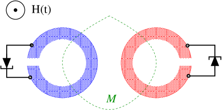
Figure 2: (Color online) Schematic of a ${\cal PT}-$symmetric metadimer comprising two tunnel diode-loaded SRRs in an alternating magnetic field $H(t)$. The SRRs are coupled magnetically through their mutual inductance $M$. Different bias in the diodes may create a balanced gain/loss structure.

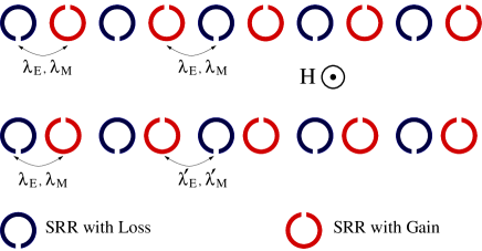
Figure 3: (Color online) Schematic of a one-dimensional ${\cal PT}-$symmetric metamaterial. Upper panel: all the split-ring resonators are equidistant. Lower panel: the separation between split-ring resonators is modulated according to a binary pattern (${\cal PT}$ dimer chain). The applied field is such that its magnetic component is perpendicular to the plane of the split-rings.

A metadimer comprising two SRRs loaded with tunnel diodes in an external alternating magnetic field is shown in Fig. 2. The equivalent circuit parameters $R$, $C$, and $L$ of the SRRs and the bias in the diodes have been adjusted so that: (i) the two elements have the same eigenfrequencies; (ii) one of the SRRs has gain while the other has equal amount of loss. Then, the pair of SRRs is a ${\cal PT}-$symmetric metadimer that can used for the construction of a one-dimensional ${\cal PT}-$symmetric metamaterial, which moreover are nonlinear due to the tunnel diodes. The alternating magnetic field induces an electromotive force (emf) in each SRR due to Faraday’s law which in turn produce currents that couple the SRRs magnetically through their mutual inductance $M$ (Fig. 2). The coupling strength between SRRs is rather weak due to the nature of their interaction (magnetoinductive), and has been calculated accurately by several authors Sydoruk2006 ; Rosanov2011 . The SRRs may also be coupled electrically, through the electric dipoles that develop in their slits. Thus, in the general case one has to consider both magnetic and electric coupling between SRRs. However, for particular relative orientations of the SRR slits the magnetic interaction is dominant, while the electric interaction can be neglected in a first approximation Hesmer2007 ; Sersic2009 ; Feth2010 . As can be seen in Fig. 3, the ${\cal PT}-$symmetric metadimers can be arranged in a one-dimensional lattice in two distinct configurations; one with all the SRRs equidistant and the other with the SRRs forming a ${\cal PT}$ dimer chain.

Within the framework of the equivalent circuit model, a set of discrete differential equations has been used to describe the dynamics in nonlinear magnetic metamaterials Lazarides2006 ; Molina2009 ; Lazarides2011 ; Rosanov2011 . Takining into account the binary structure of the ${\cal PT}$ dimer chain, the dynamics of the ${\cal PT}-$symmetric metamaterial with balanced gain and loss is governed by the following equations which are presented in normalized form Lazarides2013

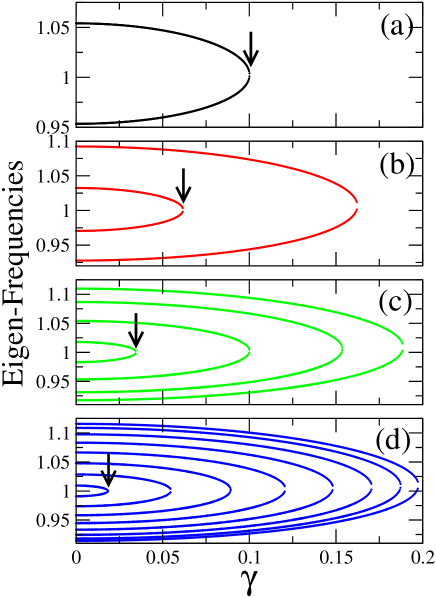
Figure 4: (Color online) Frequency eigenvalues of the free ${\cal PT}-$symmetric SRR array as a function of the gain/loss parameter $\gamma$ for $\lambda_{E}=0$, $\lambda_{M}=-0.1$, and (a) $N=2$; (b) $N=4$; (c) $N=8$; (d) $N=16$. The arrows indicate the critical point $\gamma_{c}$ for the exact-to-broken ${\cal PT}$ phase transition. Only the real eigenfrequencies is shown for clarity.

$$\lambda_{M}^{\prime}\ddot{q}_{2n}+\ddot{q}_{2n+1}+\lambda_{M}\ddot{q}_{2n+2}$$

$$+\lambda_{E}^{\prime}q_{2n}+q_{2n+1}+\lambda_{E}q_{2n+2}$$

$$+\alpha q_{2n+1}^{2}+\beta q_{2n+1}^{3}+\gamma\dot{q}_{2n+1}=\varepsilon_{0}\sin(\Omega\tau)$$ (1)

$$\lambda_{M}\ddot{q}_{2n-1}+\ddot{q}_{2n}+\lambda_{M}^{\prime}\ddot{q}_{2n+1}$$

$$+\lambda_{E}q_{2n-1}+q_{2n}+\lambda_{E}^{\prime}q_{2n+1}$$

$$+\alpha{q}_{2n}^{2}+\beta{q}_{2n}^{3}-\gamma\dot{q}_{2n}=\varepsilon_{0}\sin(\Omega\tau)$$ (2)

where $\lambda_{M},\lambda_{M}^{\prime}$ and $\lambda_{E},\lambda_{E}^{\prime}$ are the magnetic and electric coupling coefficients, respectively, with $\lambda_{E,M}>\lambda_{E,M}^{\prime}$ and $\lambda_{E,M}\lambda_{E,M}^{\prime}>0$, $\alpha$ and $\beta$ are dimensionless nonlinear coefficients, $\gamma$ is the gain/loss coefficient ($\gamma>0$), $\varepsilon_{0}$ is the amplitude of the external driving voltage, while $\Omega$ and $\tau$ are the driving frequency and temporal variable, respectively, normalized to the inductive-capacitive ($LC$) resonance frequency $\omega_{0}$ and inverse $LC$ resonance frequency $\omega_{0}^{-1}$, respectively, $\omega_{0}=1/\sqrt{LC_{0}}$ with $C_{0}$ being the linear capacitance.

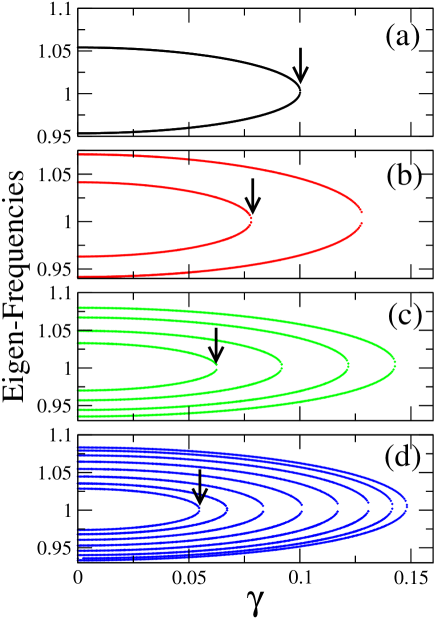
Figure 5: (Color online) Frequency eigenvalues of the free ${\cal PT}-$symmetric dimer chain as a function of the gain/loss parameter $\gamma$ for $\lambda_{E}=\lambda_{E}^{\prime}=0$, $\lambda_{M}=-0.1$, $\lambda_{M}=-0.05$, and (a) $N=2$; (b) $N=4$; (c) $N=8$; (d) $N=16$. The arrows indicate the critical point $\gamma_{c}$ for the exact-to-broken ${\cal PT}$ phase transition. Only the real eigenfrequencies are shown for clarity.

The values selected for the nonlinear coefficients $\alpha=-0.4$, $\beta=0.08$ are typical for a diode and they provide a soft on-site nonlinear potential for each metamaterial element. They can be obtained from a Taylor expansion of the capacitance-to -oltage relation of an equivalent circuit diode model, that gives a very good approximation for weakly driven systems Wang2008 ; Lazarides2011 .

III Linear Eigenfrequency Spectra and Critical Point

In order to obtain the critical value of $\gamma=\gamma_{c}$ that separates the exact ${\cal PT}-$phase, where all the eigenvalues are real, from the broken ${\cal PT}-$phase, where at least a pair of eigenvalues is complex, we calculate the frequency spectrum. This is a straightforward procedure for systems with relatively small number of SRRs; the roots of the determinant of the linearized Eqs. (II) and (II) for $\varepsilon_{0}=0$ are obtained with a root-finding algorithm and then plotted against the gain/loss parameter $\gamma$. In Figs. 4 and 5, the real eigenfrequencies of ${\cal PT}-$symmetric metamaterials in both configurations are shown as a function of $\gamma$, while the arrows indicate the critical point $\gamma_{c}$ in each case. Thus, for $\gamma<\gamma_{c}$ all eigenvalues are real, while in the opposite case at least a pair of eigenvalues has become complex. As we can see from the figures, for $\gamma>\gamma_{c}$ more and more eigenfrequency pairs become complex with increasing $\gamma$, until they all become complex for a particular value of $\gamma$. Moreover, as we can see from an inspection of Figs. 4 and 5, obtained for the equidistant SRR configuration and the ${\cal PT}$ dimer chain, respectively, the value of $\gamma_{c}$ decreases rapidly with increasing number of SRRs $N$ for the former configuration, while it tends to a constant value for the latter configuration. This can be seen more clearly in Fig. 6, where the critical point $\gamma_{c}$ is plotted as a function of $N$ for both configurations. For the curves corresponding to equidistant SRRs (corresponding to two different values of the magnetic coupling coefficient $\lambda_{M}$) we see that $\gamma_{c}$ is smaller for lower magnetic coupling coefficient $\lambda_{M}$. However, in both curves corresponding to equidistant SRRs the value of the critical point $\gamma_{c}$ tends to zero with increasing $N$. In contrast, for the ${\cal PT}$ dimer chain configuration, the value of $\gamma_{c}$ tends to a constant finite value which approximatelly equals the absolute difference of the magnetic coupling coefficients $\lambda_{M}$ and $\lambda_{M}^{\prime}$ (see below).

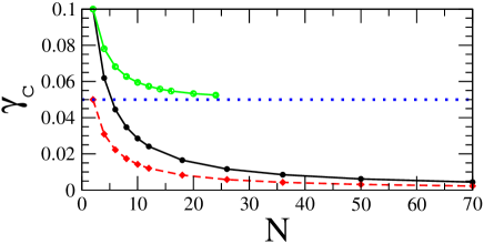
Figure 6: (Color online) Dependence of the critical gain/loss parameter value $\gamma_{c}$ on the number of SRRs, $N$, for magnetically coupled SRRs in both the equidistant and dimer chain configuration. The black squares and the red diamonds have been calculated for the former configuration with $\lambda_{M}=-0.1$ and $\lambda_{M}=-0.05$, respectively. The green circles have been calculated for the latter configuration with $\lambda_{M}=-0.1$, $\lambda_{M}^{\prime}=-0.05$. The lines serve as a guide to the eye.

For large systems, we can obtain a condition that determines the critical point $\gamma_{c}$ as a function of the magnetic coupling constant(s). In the standard way, we substitute into the linearized Eqs. (II) and (II) for $\varepsilon_{0}=0$ the trial solutions

$$q_{2n} = A\exp[i(2n\kappa-\Omega\tau)],$$ (3)

$$q_{2n+1} = B\exp\{i[(2n+1)\kappa-\Omega\tau]\},$$ (4)

where $\kappa$ is the normalized wavevector. Then, by requesting nontrivial solutions for the resulting stationary problem, we obtain

$$\Omega_{\kappa}^{2}=\left(-b\pm\sqrt{b^{2}-4ac}\right)/(2a),$$ (5)

where

$$a=1-(\lambda_{M}-\lambda_{M}^{\prime})^{2}-\mu_{\kappa}\mu_{\kappa}^{\prime},$$ (6)

$$b=\gamma^{2}-2\left[1-(\lambda_{E}-\lambda_{E}^{\prime})(\lambda_{M}-\lambda_{M}^{\prime})\right]$$

$$+\varepsilon_{\kappa}\mu_{\kappa}^{\prime}+\varepsilon_{\kappa}^{\prime}\mu_{\kappa},$$ (7)

$$c=1-(\lambda_{E}-\lambda_{E}^{\prime})^{2}-\varepsilon_{\kappa}\varepsilon_{\kappa}^{\prime},$$ (8)

and $\varepsilon_{\kappa}=2\lambda_{E}\cos(\kappa)$, $\varepsilon_{\kappa}^{\prime}=2\lambda_{E}^{\prime}\cos(\kappa)$, $\mu_{\kappa}=2\lambda_{M}\cos(\kappa)$, $\mu_{\kappa}^{\prime}=2\lambda_{M}^{\prime}\cos(\kappa)$. In the following, we neglect the electric coupling between SRRs, i.e., $\lambda_{E}=\lambda_{E}^{\prime}=0$, for simplicity. Then, Eq. (5) reduces to

$$\Omega_{\kappa}^{2}=\frac{2-\gamma^{2}\pm\sqrt{\gamma^{4}-2\gamma^{2}+(\lambda_{M}-\lambda_{M}^{\prime})^{2}+\mu_{\kappa}\mu_{\kappa}^{\prime}}}{2(1-(\lambda_{M}-\lambda_{M}^{\prime})^{2}-\mu_{\kappa}\mu_{\kappa}^{\prime})}.$$ (9)

The condition for having real $\Omega_{\kappa}$ for any $\kappa$ then reads

$$\cos^{2}(\kappa)\geq\frac{\gamma^{2}(2-\gamma^{2})-(\lambda_{M}-\lambda_{M}^{\prime})^{2}}{4\lambda_{M}\lambda_{M}^{\prime}}.$$ (10)

It is easy to see that for $\lambda_{M}=\lambda_{M}^{\prime}$ corresponding to the equidistant SRR configuration, the earlier condition cannot be satisfied for all $\kappa$’s for any positive value of the gain/loss coefficient $\gamma$, implying that a large ${\cal PT}-$symmetric SRR array (Fig. 3, upper panel) will be in the broken phase. To the contrary, for $\lambda_{M}\neq\lambda_{M}^{\prime}$, i.e., for a ${\cal PT}$ dimer chain (Fig. 3, lower panel), the above condition is satisfied for all $\kappa$’s for $\gamma\leq\gamma_{c}\simeq|\lambda_{M}-\lambda_{M}^{\prime}|$, ($\gamma^{4}\simeq 0$). In the exact phase ($\gamma<\gamma_{c}$), the ${\cal PT}-$symmetric dimer array has a gapped spectrum with two frequency bands, as shown in Fig. 7. The width of the gap separating the bands decreases with decreasing $|\lambda_{M}-\lambda_{M}^{\prime}|$ for fixed $\gamma$. For $\gamma\simeq\gamma_{c}$ the gap closes, some frequencies in the spectrum acquire an imaginary part and the ${\cal PT}$ metamaterial enters into the broken phase. Note that the gain/loss coefficient $\gamma$ has little effect on the dispersion curves of the ${\cal PT}$ dimer chain (compare with the dotted curves where $\gamma$ is set to zero), as long as the sign in front of $\gamma$ alternates from one SRR to another.

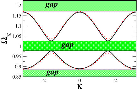
Figure 7: (Color online) Frequency bands for a ${\cal PT}-$symmetric dimer chain with balanced gain and loss for $\lambda_{M}=-0.17$, $\lambda_{M}^{\prime}=-0.10$, and $\gamma=0.05$ (black solid curves); $\gamma=0$ (red dotted curves). The gaps are indicated in green (dark) color.

IV Gain-Driven Breather Excitations

For a gapped linear spectrum, large amplitude linear modes become unstable in the presence of driving and nonlinearity. If the curvature of the dispersion curve in the region of such a mode is positive and the lattice potential is soft, large amplitude modes become unstable with respect to formation of DBs in the gap below the linear spectrum Sato2003 . For the parameters used in Fig. 7, the bottom of the lower band is located at $\Omega_{0}\simeq 0.887$, where the curvature is positive. The corresponding period at the bottom of the lower band is $T_{0}=2\pi/\Omega_{0}$. Moreover, the SRRs are subjected to soft on-site potentials for the selected values of the nonlinear coefficients $\alpha$ and $\beta$. Then, DBs can be generated spontaneously by a frequency chirped alternating driver; after turning off the driver, the breathers are driven solely by gain. A similar procedure has been applied succesfuly to lossy nonlinear metamaterials with a binary structure Molina2009 ; Lazarides2009 ; Lazarides2010a The results are illustrated in Figs. 8 and 9, where the case of a slight imbalance between gain and loss and its effect on breather generation has been also considered. In these figures, a density plot of the local energy $E_{n}$ of a ${\cal PT}-$symmetric metamaterial is shown on the $n-\tau$ plane for two different values of the driving amplitude $\varepsilon_{0}$.

In the following, the integration of Eqs. (II) and (II) implemented with the boundary condition

$$q_{0}(\tau)=q_{N+1}(\tau)=0,$$ (11)

that accounts for the termination of the structure in finite systems, is performed with a 4th order Runge-Kutta algorithm with fixed time-step. In order to prevent instabilities that will result in divergence of the energy at particular sites in finite time, we consider a longer dimer chain with total number of SRRs $N+2N_{\ell}$; then we replace the gain with equivalent amount of loss at exactly $N_{\ell}$ SRRs at each end of the extended chain. In other words, we embbed the ${\cal PT}-$symmetric dimer chain into a geometrically identical lossy chain, in order to help the excess energy to go smothly away during evolution living behind stable (or at least very long-lived) breather structures.

We use the following procedure described in detail in Ref. Lazarides2013 :

$\bullet$ At time $\tau=0$, we start integrating Eqs. (II) and (II) from zero initial state without external driving for $500~{}T_{0}\simeq 3500$ time units (t.u.) to allow for significant developement of large amplitude modes.

$\bullet$ At time $\tau\simeq 3500$ t.u. the driver is switched-on with low-amplitude $\varepsilon_{0}$ and frequency slightly above $\Omega_{0}$ ($1.01~{}\Omega_{0}\simeq 0.894$). The frequency is then chirped downwards with time to induce instability for the next $10600$ t.u. ($\sim 1500~{}T_{0}$), until it is well below $\Omega_{0}$ ($0.997~{}\Omega_{0}\simeq 0.882$). During that phase, a large number of excitations are generated that move and strongly interact to each other, eventually merging into a small number of high amplitude breathers and multi-breathers.

$\bullet$ At time $\tau\simeq 14100$ t.u. (point A on Figs. 8 and 9), the driver is switched off and the DBs that have formed are solely driven by the gain. They continue to interact for some time until they reach an apparently stationary state and get trapped at particular sites. The high density segments between the points A and C in Figs. 8 and 9 precisely depict those gain-driven DB structures.

$\bullet$ At time $\tau\sim 440000$ t.u. (point C on Figs. 8 and 9), the gain is replaced everywhere by equal amount of loss, and the breathers die out rapidly.

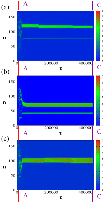
Figure 8: (Color online) Spatiotemporal evolution of the energy density $E_{n}$ for a ${\cal PT}-$symmetric dimer chain with $N=70$, $N_{\ell}=10$, $\Omega_{0}=0.887$, $\gamma=0.002$, $\lambda_{M}=-0.17$, $\lambda_{M}^{\prime}=-0.10$ ($\lambda_{E}=\lambda_{E}^{\prime}=0$), $\varepsilon_{0}=0.085$, $\gamma=0.002$ and (a) excess loss $0.2\%$; (b) balanced case; (c) excess gain $0.2\%$.

Note that the above procedure of breather generation is very sensitive to parameter variations of the external fields. Even though the values of the driving amplitudes in Figs. 8 and 9 are rather close (i.e., $\varepsilon_{0}=0.085$ and $0.095$, respectively), the breather structures as well as their numbers are different. In Fig. 8(b), in the balanced gain/loss case, we observe two distinct structures that have been formed that correspond to a relatively high amplitude multi-breather and a low amplitude breather. These structures remain stationary during the long time interval they have been followed ($>56000~{}T_{0}$). In Figs. 8(a) and 8(c), gain and loss are not perfectly matched; in Fig. 8(a) loss exceeds gain by a small amount while in in Fig. 8(c) gain exceeds loss by the same small amount. Notably, breather excitations may still be formed through the frequency chirping procedure in the presence of a small amount of either net gain or net loss. Indeed, as we may observe comparing Figs. 8(a) and 8(c) with Fig. 8(b), the same structures are formed [except the low amplitude breather that is not visible in Fig. 8(c)]. However, both in Figs. 8(a) and 8(c) we can see a slow gradual widening of the high amplitude multibreather: when loss exceeds gain the multibreather losses its energy at a low rate, with its excited sites that are closer to its end-points gradually falling down to a low amplitude state. Similarly, when gain exceeds loss, the high amplitude multibreather slowly gains energy and becomes wider. In both cases, breather destruction will take place in a time-scale that depends exponentially on the gain/loss imbalance. Thus, in an experimental situation, where gain/loss balance is only approximate, it will be still possible to observe breathers at relatively short time-scales. Similar observations hold for Fig. 9 as well. In this figure, we observe three relatively high amplitude multibreather structures that are formed both in the balanced and the imbalanced case. Here we also observe that instabilities may appear after long time intervals of apparently stationary breather evolution as well. Whenever this happens, they start moving through the lattice until they get once more trapped at different lattice sites. In Fig. 9(b) such an instability appears between $~{}200000-250000$ t.u. for the two narrower multibreather structures. The one of them gets trapped a few tenths lattice sites away from its previous position, while the other (the narrowest) collides and it is absorbed by the wide multibreather located at $n~{}50$.

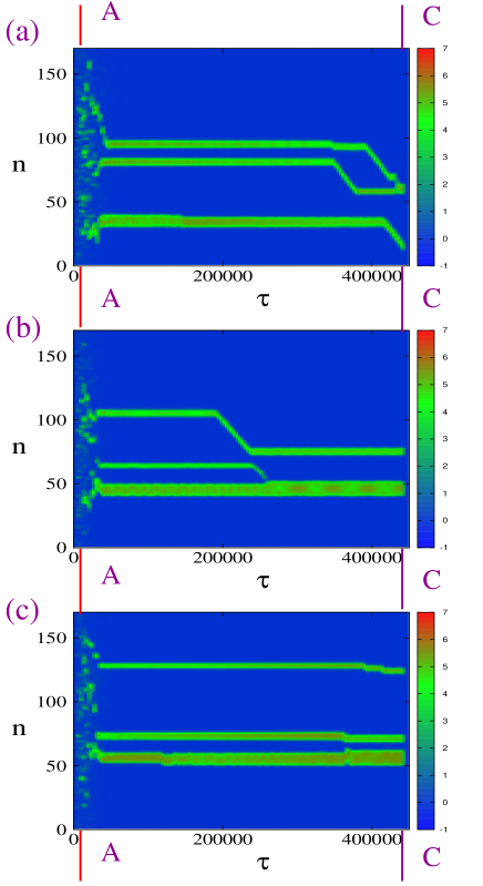
Figure 9: (Color online) Spatiotemporal evolution of the energy density $E_{n}$ for a ${\cal PT}-$symmetric dimer chain with $N=70$, $N_{\ell}=10$, $\Omega_{0}=0.887$, $\gamma=0.002$, $\lambda_{M}=-0.17$, $\lambda_{M}^{\prime}=-0.10$ ($\lambda_{E}=\lambda_{E}^{\prime}=0$), $\varepsilon_{0}=0.095$, $\gamma=0.002$ and (a) excess loss $0.2\%$; (b) balanced case; (c) excess gain $0.2\%$.

V Classical ${\cal PT}-$Symmetry in Zero Dimensions

In the classical domain, in all cases of ${\cal PT}-$symmetric systems investigated so far, the combination of time-reversal and parity symmetries is utilized: In a given time-evolution if we reverse time while ”reflecting” position and momentum, we must retrace the original path. The parity operation requires that the system is extended either in continuous or discrete space in order to be able to perform this operation. We show here that this is not necessary and that the features of the ${\cal PT}$ -symmetric systems can be preserved in ”zero” dimensions where the parity symmetry is trivial.

We consider the following simple harmonic oscillator:

$$\ddot{x}+2\theta(t)\dot{x}+\omega_{0}^{2}x=0,$$ (12)

where $x\equiv x(t)$ is the equilibrium dislacement of a mass (the charge in an $RLC$ cirquit), $\omega_{0}$ the resonant oscillation frequency while $\theta(t)$ is a time-dependent ”damping” term; both $\omega_{0}$ and $\theta(t)$ are scaled to the mass (impedance of the circuit). We take $\theta(t)$ to be periodic with period $T$, viz. $\theta(t+T)=\theta(t)$ while its values may be both positive and negative, i.e., for some part of the period the oscillator experiences damping while in the rest of the period time amplification, or anti-damping. We investigate the osillator evolution after long time and the stability of the motion. Instead of addressing a general periodic function $\theta(t)$ we focus on a simple form that makes the problem readily solvable, viz. we take

$$\theta(t)=\left\{\begin{array}[]{ll}+\gamma&\mbox{if $0\leq t<\tau_{1}$};\\ -\gamma&\mbox{if $\tau_{1}\leq t<\tau_{2}$}.\end{array}\right.$$ (13)

where $T=\tau_{1}+\tau_{2}$ and taking the plus (minus) sign in front of the coefficient $\gamma$ ($\gamma$ is defined as a positive constant, $\gamma>0$, that may assume any value between zero and unity) we have in the first (second) part of the cycle loss (gain). With this form of piecewise constant function $\theta(t)$ we can easily solve Eq. (12) for the loss (L) segment of time duration $\tau_{1}$ and gain (G) segment of duration $\tau_{2}$. The form of Eq. (13) permits to view the problem as mapping of the position-velocity vector at a given time to the position-velocity vector at a later time; if in the begining of the gain (loss) period (assuming $t=0$) we have position and velocity equal to $(x_{0},~{}\dot{x}_{0})$. Then after the evolution during time $\tau$ ($\tau_{1}$ or $\tau_{2}$, respectively) we obtain:

$$\left(\begin{array}[]{c}x\\ \dot{x}\end{array}\right)=M_{G/L}(\tau)\left(\begin{array}[]{c}x_{0}\\ \dot{x_{0}}\end{array}\right)$$ (14)

where for gain we have

$$M_{G}(\tau_{1})=\frac{e^{\gamma\tau_{1}}}{\delta}\times$$

$$\left(\begin{array}[]{cc}\delta\cos\delta\tau_{1}-\gamma\sin\delta\tau_{1}&\sin\delta\tau_{1}\\ -\omega_{0}^{2}\sin\delta\tau_{1}&\delta\cos\delta\tau_{1}+\gamma\sin\delta\tau_{1}\end{array}\right)$$ (17)

and for the loss respectively

$$M_{L}(\tau_{1})=\frac{e^{-\gamma\tau_{2}}}{\delta}\times$$

$$\left(\begin{array}[]{cc}\delta\cos\delta\tau_{2}+\gamma\sin\delta\tau_{2}&\sin\delta\tau_{2}\\ -\omega_{0}^{2}\sin\delta\tau_{2}&\delta\cos\delta\tau_{1}-\gamma\sin\delta\tau_{2}\end{array}\right)$$ (20)

where $\delta=\sqrt{\omega_{0}^{2}-\gamma^{2}}$. Using the mapping, we may obtain long time evolution after $N$ periods $T$ as a repetitive application of the matrices $M_{G}(\tau_{1})$ and $M_{L}(\tau_{2})$ to an arbitraty initial state $(x_{0},~{}\dot{x}_{0})$. Since the matrices $M_{L/G}(\tau)e^{\pm\gamma\tau}$ are unimodular, the long time evolution with be dominated by the exponential term $\exp[N\gamma(\tau_{1}-\tau_{2})]$; this leads trivially to exponential growth ($\tau_{1}>\tau_{2}$) or exponential decay ($\tau_{1}<\tau_{2}$). As a result we consider the more interesting case with $\tau_{1}=\tau_{2}=\tau\equiv T/2$; in this case the gain and loss power is perfectly matched during the period $T$. The combined propagation matrix after one period (assuming first gain) is simply $M(T)=M_{L}(\tau)M_{G}(\tau)$, i.e.,‘

$$M(T)=\frac{1}{\delta^{2}}\left(\begin{array}[]{cc}M_{11}&M_{12}\\ M_{21}&M_{22}\end{array}\right)$$ (21)

where $M_{ij}$ are given by

$$M_{11}=-\gamma^{2}+\omega_{0}^{2}\cos(2\phi),$$ (22)

$$M_{12}=+2\sin\phi(\delta\cos\phi+\gamma\sin\phi)$$ (23)

$$M_{21}=-2\omega_{0}^{2}\sin\phi(\delta\cos\phi-\gamma\sin\phi)$$ (24)

$$M_{22}=-\gamma^{2}+\omega_{0}^{2}\cos(2\phi)$$ (25)

and $\phi=\delta\tau\equiv\delta T/2$. The matrix $M$ is clearly also unimodular with eigenvalues $e^{i\mu}$ and $e^{-i\mu}$; since the trace of a matrix is invariant we find

$$\cos\mu=\frac{-\gamma^{2}+\omega_{0}^{2}\cos 2\phi}{\delta^{2}}.$$ (26)

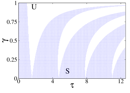
Figure 10: (Color online) Phase diagram on the $\gamma-\tau$ plane for the harmonic oscillator with time-dependent ”damping” term, obtained from Eq. (34). The stability region is indicated in blue (dark) color.

Stability Equation.- Eq. (26) can be re written as

$$\cos\mu=\frac{1-B^{2}\cos 2\phi}{1-B^{2}}=1+\frac{2B^{2}\sin^{2}\phi}{1-B^{2}}$$ (27)

with $B=\frac{\omega_{0}}{\gamma}$. In order to have stable motion it is necessary that $|\cos\mu|\leq 1$, or $-1\leq 1+\frac{2B^{2}\sin^{2}\phi}{1-B^{2}}\geq 1$, leading to

$$-2\leq\frac{2B^{2}\sin^{2}\phi}{1-B^{2}}\leq 1$$ (28)

Eq. (28) has solutions only for $|B|>1$ or $|\gamma|<\omega_{0}$, for $\omega_{0}>0$; in the latter case we find

$$|\cos\phi|\geq\left|\frac{\gamma}{\omega_{0}}\right|$$ (29)

The range thus of allowed values for the angle $\phi$ ($\gamma>0$) is

$$\frac{\gamma}{\omega_{0}}\leq\cos\phi\leq 1$$

$$-1\leq\cos\phi\leq-\frac{\gamma}{\omega_{0}}$$ (30)

We note that there are multiple allowed solutions marked by the the lines $\cos\phi=\pm\gamma/\omega_{0}$, i.e., for the three parameters of the problem $\gamma$, $T=2\tau$ and $\omega_{0}$ the transcedental equation

$$\cos(\delta\tau)=\left\{\begin{array}[]{ll}+\frac{\gamma}{\omega_{0}}&\mbox{for $2n\pi-\pi/2<\delta\tau<2n\pi+\pi/2$};\\ -\frac{\gamma}{\omega_{0}}&\mbox{for $2\pi n+\pi/2<\delta\tau<2\pi n+3\pi/2$},\end{array}\right.$$ (33)

where $n=0,\pm 1,\pm 2,..$, marks the onset of the transition from stable to unstable evolution. This is the equivalent to the ${\cal PT}$ transition from the exact (stable) to the broken (unstable) phase in this zero-dimensional problem. Using Eq. (29) we construct a ${\cal PT}$ phase diagram on the $\tau-\gamma$ plane (Fig. 10), where the blue (dark) color indicates regions of stability. If we fix one of the parameters, variation of the other drives the oscillator through alternatingly stable and unstable regions, as can be readily observed from Fig. 10.

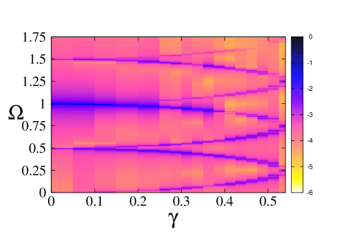
Figure 11: (Color online) Density plot of the logarithm of the frequency spectra of $x(t)$, $y=\log_{10}\{PS[x(t)]\}$, as a function of $\gamma$. The discrete frequency components of the spectra for each value of $\gamma$ are indicated with blue (darker) color.

Introducing the frequency $\omega=2\pi/T\equiv\pi/\tau$ we define the reduced parameters $\Omega=\omega/\omega_{0}$ and $\tilde{\gamma}=\gamma/\omega_{0}$. Then, the equation that controls the stability regions becomes

$$\left|\cos\left[\frac{\pi\sqrt{1-\gamma^{2}}}{\Omega}\right]\right|=\gamma,$$ (34)

where the tilde has been dropped. Eq. (34) has solutions for $|\gamma|<1$; for different reduced frequencies $\Omega$ we obtain different number of solutions of the earlier equation, the number of the latter icreases with decreasing frequency $\omega$. Once we have the solutions of Eq. (34) we can find the regimes of stability and instability. Consider the resonant case $\Omega=1$ where the external frequency of gain/loss alternation matches the self-frequency of the oscillator. Besides the trivial solution at $\gamma=0$, numerical solution of Eq. (34) gives $\gamma_{1}\approx 0.676$ so that the stable region is in the range $0\leq\gamma\leq\gamma_{1}$. For $\Omega=0.5$ the corresponding solutions are $\gamma_{1}\approx 0.54$, $\gamma_{2}\approx 0.80$, and $\gamma_{3}\approx 0.90$ with two stability regions, i.e., $0\leq\gamma\leq\gamma_{1}$ and $\gamma_{2}\leq\gamma\leq\gamma_{3}$.

The stable solutions of Eq. (12) as a function of time $t$ are in general quasi-periodic oscillations whose spectral content varies both with $\tau$ and $\gamma$. For an illustration, we consider a particular value of $\tau$, i.e., $\tau=2\pi$ ($\Omega=0.5$) for which the boundaries of the stability regions have been calculated. For the interval with relatively low values of $\gamma$, $0\leq\gamma\leq\gamma_{1}\simeq 0.54$, that is more physically relevant, we present a density plot of the logarithm of the frequency spectra of $x(t)$, $y=\log_{10}\{PS[x(t)]\}$, as a function of $\gamma$ (Fig. 11). In this figure, the discrete frequency components of the spectra for each value of $\gamma$ are indicated in dark (blue) color. For $\gamma=0$ and very close to zero, the only frequency appearing in the spectrum is the eigenfrequency of the oscillator $\Omega\simeq 1$. With increasing $\gamma$, the frequency components at $\Omega\simeq 1\pm 0.5$ become more and more important. At about $\gamma=0.15$ these half-integer frequency components start splitting into pairs of frequencies that are symmetric around the half-integer values. The separation between these pairs increases with further increasing $\gamma$, and the frequency components from neighboring pairs come closer and closer together until they eventually merge for $\gamma$ approaching its critical value $0.54$.

VI Conclusions

We have investigated theoretically a ${\cal PT}-$symmetric nonlinear metamaterial relying on gain and loss. Eigenfrequency spectra for linearized systems of either small and large $N$ and two different configurations were calculated and the critical points $\gamma_{c}$ were determined. Large ${\cal PT}-$symmetric metamaterials with the dimer chain configuration exhibit phase transitions for the exact to the broken ${\cal PT}-$symmetry phase, while large ${\cal PT}-$symmetric metamaterials with the equidistant SRR configuration are always in the broken ${\cal PT}$ phase.

In the presence of nonlinearity, we have demonstrated numerically the a ${\cal PT}-$symmetric dimer chain supports localized excitations in the form of discrete breathers. Breathers are excited by a purely dynamical process, with a frequency chirped external magnetic field that induces instability in a zero initial state. Subsequently, the nonlinearity focuses energy around points that have acquired high amplitude leading to the formation of localized structures. The external field is then switched off and those localized structures are then solely driven by the gain, while the excess energy lives the system through its lossy parts at the ends, leading eventually to breather generation.

Remarkably, slight imbalance between gain and loss does not destroy the breathers instantly; they can still be generated through the frequency chirping procedure and they can be regarded as stationary for relatively short time intervals. In the long term, the imbalanced breathers either gain constantly energy and diverge or lose constantly energy and vanish. The time-scale for the latter events depends exponentially on the amount of imbalance.

We have introduced a ”zero-dimensional” ${\cal PT}$ system that can be realized by a harmonic oscillator with a ”damping” term that provides balanced gain and loss, through alternation of the sign of the damping coefficient. We consider a piecewise linear gain/loss function and obtain a stability condition, i.e., a relation between the parameters of the problem. We thus obtain a ”phase diagram” with parameter regions where oscillatory (stable) motion and diverging (unstable) motion occur. A crossing of the stability boundary marks the onset of a transition from stable to unstable evolution that is equivalent to the ${\cal PT}$ transition from the exact to the broken phase in this zero-dimensional problem.

References

- (1) Achilleos, V., Kevrekidis, P.G., Frantzeskakis, D.J., Carretero-González, R.: Dark solitons and vortices in pt-symmetric nonlinear media: From spontaneous symmetry breaking to nonlinear pt phase transitions. Phys. Rev. A 86, 013,808 (7pp) (2012)
- (2) Alexeeva, N.V., Barashenkov, I.V., Sukhorukov, A.A., Kivshar, Y.S.: Optical solitons in pt-symmetric nonlinear couplers with gain and loss. Phys. Rev. A 85, 063,837 (13pp) (2012)
- (3) Anlage, S.M.: The physics and applications of superconducting metamaterials. J. Opt. 13, 024,001–10 (2011)
- (4) Barashenkov, I.V., Suchkov, S.V., Sukhorukov, A.A., Dmitriev, S.V., Kivshar, Y.S.: Breathers in pt-symmetric optical couplers. Phys. Rev. A 86, 053,809 (12pp) (2012)
- (5) Boardman, A.D., Grimalsky, V.V., Kivshar, Y.S., Koshevaya, S.V., Lapine, M., Litchinitser, N.M., Malnev, V.N., Noginov, M., Rapoport, Y.G., Shalaev, V.M.: Active and tunable metamaterials. Laser Photonics Rev. 5 (2), 287–307 (2010)
- (6) Boardman, D., King, N., Rapoport, Y.: Circuit model of gain in metamaterials. In: C. Denz, S. Flach, Y.S. Kivshar (eds.) Nonlinearities in Periodic Structures and Metamaterials, Springer Series in Optical Sciences, vol. 150, pp. 259–272. Springer Berlin, Heidelberg (2010)
- (7) Dmitriev, S.V., Sukhorukov, A.A., Kivshar, Y.S.: Binary parity-time-symmetric nonlinear lattices with balanced gain and loss. Opt. Lett. 35, 2976–2978 (2010)
- (8) El-Ganainy, R., Makris, K.G., Christodoulides, D.N., Musslimani, Z.H.: Theory of coupled optical pt-symmetric structures. Opt. Lett. 32, 2632–2634 (2007)
- (9) Esaki, L.: New phenomenon in narrow germanium junctions. Phys. Rep. 109, 603–605 (1958)
- (10) Feth, N., König, M., Husnik, M., Stannigel, K., Niegemann, J., Busch, K., Wegener, M., Linden, S.: Electromagnetic interaction of spit-ring resonators: The role of separation and relative orientation. Opt. Express 18, 6545–6554 (2010)
- (11) Flach, S., Gorbach, A.V.: Discrete breathers - advances in theory and applications. Phys. Rep. 467, 1–116 (2008)
- (12) Guo, A.: Observation of pt-symmetry breaking in complex optical potentials. Phys. Rev. Lett. 103, 093,902 (2009)
- (13) Hesmer, F., Tatartschuk, E., Zhuromskyy, O., Radkovskaya, A.A., Shamonin, M., Hao, T., Stevens, C.J., Faulkner, G., Edwardds, D.J., Shamonina, E.: Coupling mechanisms for split-ring resonators:theory and experiment. Phys. Stat. Sol. (b) 244, 1170–1175 (2007)
- (14) Hook, D.W.: Non-hermittian potentials and real eigenvalues. Ann. Phys. (Berlin) 524 (6-7), A106 (2012)
- (15) Jiang, T., Chang, K., Si, L.M., Ran, L., Xin, H.: Active microwave negative-index metamaterial transmission line with gain. Phys. Rev. Lett. 107, 205,503 (2011)
- (16) Lazarides, N., Eleftheriou, M., Tsironis, G.P.: Discrete breathers in nonlinear magnetic metamaterials. Phys. Rev. Lett. 97, 157,406–4 (2006)
- (17) Lazarides, N., Molina, M.I., Tsironis, G.P.: Breather induction by modulational instability in binary metamaterials. Acta Physica Polonica A 116 (4), 635–637 (2009)
- (18) Lazarides, N., Molina, M.I., Tsironis, G.P.: Breathers in one-dimensional binary metamaterial models. Physica B 405, 3007–3011 (2010)
- (19) Lazarides, N., Paltoglou, V., Tsironis, G.P.: Nonlinear magnetoinductive transmission lines. Int. J. Bifurcation Chaos 21, 2147–2156 (2011)
- (20) Lazarides, N., Tsironis, G.P.: Gain-driven discrete breathers in pt-symmetric nonlinear metamaterials. Phys. Rev. Lett. 110, 053,901 (5pp) (2013)
- (21) Li, K., Kevrekidis, P.G.: Pt-symmetric oligomers: Analytical solutions, linear stability, and nonlinear dynamics. Phys. Rev. E 83, 066,608 (7pp) (2011)
- (22) Lin, Z., Ramezani, H., Eichekraut, T., Kottos, T., Cao, H., Christodoulides, D.N.: Unidirectional invisibility induced by pt-symmetric periodic structures. Phys. Rev. Lett. 106, 213,901 (4pp) (2011)
- (23) Makris, K.G., El-Ganainy, R., Christodoulides, D.N., Musslimani, Z.H.: Beam dynamics in pt-symmetric optical lattices. Phys. Rev. Lett. 100, 103,904 (2008)
- (24) Miroshnichenko, A.E., Malomed, B.A., Kivshar, Y.S.: Nonlinearly pt-symmetric systems: Spontaneous symmetry breaking and transmission resonances. Phys. Rev. A 84, 012,123 (4pp) (2011)
- (25) Molina, M.I., Lazarides, N., Tsironis, G.P.: Bulk and surface magnetoinductive breathers in binary metamaterials. Phys. Rev. E 80, 046,605 (2009)
- (26) Ramezani, H., Christodoulides, D.N., Kovanis, V., Vitebskiy, I., Kottos, T.: Pt-symmetric talbot effects. Phys. Rev. Lett. 109, 033,902 (2012)
- (27) Ramezani, H., Kottos, T., El-Ganainy, R., Christodoulides, D.N.: Unidirectional nonlinear pt-symmetric optical structures. Phys. Rev. A 82, 043,803 (6pp) (2010)
- (28) Rosanov, N.N., Vysotina, N.V., Shatsev, A.N., Shadrivov, I.V., Powell, D.A., Kivshar, Y.S.: Discrete dissipative localized modes in nonlinear magnetic metamaterials. Opt. Express 19, 26,500 (2011)
- (29) Rüter, C.E., Makris, K.G., El-Ganainy, R., Christodoulides, D.N., Segev, M., Kip, D.: Observation of parity–time symmetry in optics. Nature Physics 6, 192– (2010)
- (30) Sato, M., Hubbard, B.E., Sievers, A.J., Ilic, B., Czaplewski, D.A., Graighead, H.G.: Observation of locked intrinsic localized vibrational modes in a micromechanical oscillator array. Phys. Rev. Lett. 90, 044,102 (4pp) (2003)
- (31) Schindler, J., Li, A., Zheng, M.C., Ellis, F.M., Kottos, T.: Experimental study of active lrc circuits with pt symmetries. Phys. Rev. A 84, 040,101(R) (2011)
- (32) Sersić, I., Frimmer, M., Verhagen, E., Koenderink, A.F.: Electric and magnetic dipole coupling in near-infrared split-ring metamaterial arrays. Phys. Rev. Lett. 103, 213,902 (2009)
- (33) Si, L.M., Jiang, T., Chang, K., T.-C.Chen, Lv, X., Ran, L., Xin, H.: Active microwave metamaterials incorporating ideal gain devices. Materials 4, 73–83 (2011)
- (34) Suchkov, S.V., Malomed, B.A., Dmitriev, S.V., Kivshar, Y.S.: Solitons in a chain of parity-time invariant dimers. Phys. Rev. A 84, 046,609 (2011)
- (35) Sydoruk, O., Radkovskaya, A., Zhuromskyy, O., Shamonina, E., Shamonin, M., Stevens, C., Faulkner, G., Edwards, D., Solymar, L.: Tailoring the near-field guiding properties of magnetic metamaterials with two resonant elements per unit cell. Phys. Rev. B 73, 224,406 (2006)
- (36) Szameit, A., Rechtsman, M.C., Bahat-Treidel, O., Segev, M.: Pt-symmetry in honeycomb photonic lattices. Phys. Rev. A 84, 021,806(R) (2011)
- (37) Wang, B., Zhou, J., Koschny, T., Soukoulis, C.M.: Nonlinear properties of split-ring resonators. Opt. Express 16, 16,058 (2008)
- (38) Xu, W., Padilla, W.J., Sonkusale, S.: Loss compensation in metamaterials through embedding of active transistor based negative differential resistance circuits. Opt. Express 20, 22,406 (2012)
- (39) Zezyulin, D.A., Konotop, V.V.: Nonlinear modes in finite-dimensional pt-symmetric systems. Phys. Rev. Lett. 108, 213,906 (5pp) (2012)
- (40) Zheludev, N.I.: The road ahead for metamaterials. Science 328, 582–583 (2010)