An exact formalism for the quench dynamics of integrable models

Abstract

We describe a formulation for studying the quench dynamics of integrable systems generalizing an approach by Yudson. We study the evolution of the Lieb-Liniger model, a gas of interacting bosons moving on the continuous infinite line and interacting via a short range potential. The formalism allows us to quench the system from any initial state. We find that for any value of repulsive coupling independently of the initial state the system asymptotes towards a strongly repulsive gas, while for any value of attractive coupling, the system forms a maximal bound state that dominates at longer times. In either case the system equilibrates but does not thermalize. We compare this to quenches in a Bose-Hubbard lattice and show that there, initial states determine long-time dynamics independent of the sign of the coupling.

I Introduction

Nonequilibrium processes occur in fields as diverse as metallurgy and cell biology – in fact, most physical processes that occur in nature are dynamical. It is therefore important to understand nonequilibrium phenomena from a variety of perspectives and in several different contexts.

In the context of physics, the dynamics of nonequilibrium processes has been studied since the early days of thermodynamics (see Ref. De Groot and Mazur, 2012 for a historical introduction to the subject). More recently, the study of quantum nonequilibrium processes has received a boost from highly tunable experimental systems, in particular ultracold atomic gases, that can be well isolated from their environment. They provide a testing ground for theories of quantum nonequilibrium behavior and have led to observations of interesting new phenomena Bloch et al. (2008).

Unlike thermodynamics, there exists no general framework to understand far from equilibrium behavior. Different problems need different approaches and in most cases we can only understand the behavior of physical observables in limited regimes of parameters or windows of time. However, a good sense of the complexity of the problem is emerging from a multitude of studies on several types of systems analytically, computationally, and experimentally.

Within the domain of quantum phenomena, transport and quenches are the primary means of studying nonequilibrium physics. Transport phenomena include for example, transient and steady-state currents in devices, study of quantum impurity models and their conduction properties, quantum hall edge states, and the surface states of topological insulators. Quenches, on the other hand, allow us to study phenomena like thermalization and relaxation of physical observables by strongly disturbing an equilibrium system and watching it evolve . Cold atom systems, as noted, are particularly amenable to quenches – we briefly describe these in section II. On the theoretical side, with advances in computational techniques, it is possible to calculate the time evolution of various observables of larger systems and study the underlying physics Rigol (2009); Rigol et al. (2008); Calabrese and Caux (2007); Mossel and Caux (2012); White and Feiguin (2004); Daley et al. (2004). However, these techniques are not suitable for very large systems or continuum models.

In this article, we are interested in studying the quench dynamics of systems described by integrable models. These models possess an infinite number of conserved quantities, and this property is expected to reveal itself in their dynamics Rigol (2009); Rigol et al. (2008); Kinoshita et al. (2006). A generic model would access all of the constant energy surface in phase space as it evolves, but this may not be the case for an integrable model. As we will mention later in more detail, this work studies the expansion of a local initial state into infinite volume, and therefore is different from studying the thermodynamics. The approach we take here mimics experiments directly.

The eigenstates of integrable models can be obtained via the Bethe Ansatz technique Bethe (1931), which allows the construction of a complete set of eigenstates of the Hamiltonian. The Bethe Ansatz has proved to be of tremendous use in studying the ground states and thermodynamics of such models Takahashi (1999); Andrei et al. (1983); Tsvelick and Wiegmann (1983); Andrei (1995). However, in spite of knowing the eigenstates of the Hamiltonian the dynamics still remains a complicated problem. In the remainder of this paper, we elucidate a framework for dynamics introduced by Yudson Yudson (1985, 1988). We introduce some generalizations and use it to understand the quench dynamics of a gas of bosons with attractive or repulsive short range interactions in the context of the Lieb-Liniger model Lieb and Liniger (1963). This approach allows analytical calculations that are essential for a complete understanding of the out-of-equilibrium properties of the system.

The article is a follow up to Ref. Iyer and Andrei, 2012. Some of the formulas are derived in detail, and some of the plots are repeated for completeness. We also correct an error in the earlier work.

Before getting into details we discuss some general issues concerning the quench dynamics of isolated systems defined on the infinite line.

I.1 Dynamics of $1d$ isolated many-body systems

While studying the thermodynamic properties of a quantum system, one needs to enumerate and classify the eigenstates of the Hamiltonian in order to construct the partition function. To achieve this, some finite volume boundary conditions (BC) are typically imposed — either periodic BC to maintain translation invariance or open BC when the system has physical ends. One can then identify the ground state and the low lying excitations that dominate the low-temperature physics. In the thermodynamic limit $\frac{N\to\infty}{L\to\infty}\equiv\rho$, the limit of very large systems with large number of particles at finite density, the effect of the boundary condition is negligible and we expect the results to be universally valid.

When the system is out of equilibrium, a different set of issues arises. We shall consider here the process of a “quantum quench” where one studies the time evolution of a system after a sudden change in the parameters of the Hamiltonian governing the system. To be precise, one assumes that the system starts in some stationary state $\lvert\Psi_{0}\rangle$. This stationary state can be thought of as the ground state of some (interacting) Hamiltonian $H_{0}$. Following the quench at $t=0$, the system evolves in time under the influence of a new Hamiltonian $H$ which may differ from $H_{0}$ in many ways. One may add an interaction, change an interaction coupling constant, apply or remove an external potential or increase the size of the system. Further, the quench can be sudden, i.e., over a time window much shorter than other time scales in the system, driven at a constant rate or with a time dependent ramp.

In this paper we shall concentrate on sudden quenches where the initial state $\lvert\Psi_{0}\rangle$ describes a system in a finite region of space with a particular density profile: lattice-like, or condensate-like (see Fig. 1). Under the effect of the quenched Hamiltonian the system evolves as $\lvert\Psi_{0},t\rangle=e^{-iHt}\lvert\Psi_{0}\rangle$.

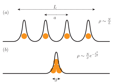
Figure 1: Initial states. $(a)$ For $\frac{a}{\sigma}\gg 1$, we have a lattice like state, $\lvert\Psi_{\text{latt}}\rangle$. $(b)$ For $a=0$, we have a condensate like state $\lvert\Psi_{\text{cond}}\rangle$, $\sigma$ determines the spread.

To compute the evolution, it is convenient to expand the initial state in the eigenbasis of the evolution Hamiltonian,

$$\lvert\Psi_{0}\rangle=\sum_{\{n\}}C_{n}\lvert n\rangle,$$ (I.1)

where $\lvert n\rangle$ are the eigenstates of $H$ and $C_{n}=\langle n\rvert\Psi_{0}\rangle$ are the overlaps with the initial state, determining the weights with which different eigenstates contribute to the time evolution:

$$\lvert\Psi_{0},t\rangle=\sum_{\{n\}}e^{-i\epsilon_{n}t}C_{n}\lvert n\rangle.$$ (I.2)

The evolution of observables is then given by,

$$\begin{split}\langle\hat{O}(t)\rangle_{\Psi_{0}}&=\langle\Psi_{0},t|\hat{O}\lvert\Psi_{0},t\rangle\\ &=\sum_{\{n,m\}}e^{-i(\epsilon_{m}-\epsilon_{n})t}C^{*}_{n}\,C_{m}\langle n|\hat{O}\lvert m\rangle,\end{split}$$ (I.3)

with observables that may be local operators, correlation functions, currents or global quantities such as entanglements.

The time evolution is characterized by the energy of the initial state,

$$\epsilon_{\text{quench}}=\langle\Psi_{0}\rvert H\lvert\Psi_{0}\rangle=\sum_{\{n\}}\epsilon_{n}\lvert C_{n}\rvert^{2}$$ (I.4)

which is conserved throughout the evolution, specifying the energy surface on which the system moves. This surface is determined by the initial state through the overlaps $C_{n}$. Unlike the situation in thermodynamics where the ground state and low-lying excitations play a central role, this is not the case out-of-equilibrium. A quench puts energy into the system which the isolated system cannot dissipate and it cannot relax to its ground state. Rather, the eigenstates that contribute to the dynamics depend strongly on the initial state via the overlaps $C_{n}$ (see Fig. 2).

A vivid illustration comes from comparing quenches in systems that differ in the sign of the interaction. In the Bose-Hubbard model and the XXZ model it has been observed that the sign of the interaction plays no role in the quench dynamics Lahini et al. (2012); Barmettler et al. (2010), even though the ground states that correspond to the different signs are very different. For example, for the XXZ magnet, the ground state is either ferromagnetic or Néel ordered (RVB in 1$d$) depending on the sign of the anisotropy $\Delta$. In Appendix A, we show results for the Bose-Hubbard model, and provide an argument for this observation. The Lieb-Liniger model, whose quench dynamics we describe here, on the other hand shows very different behavior, reaching an long time equilibrium state that depends mainly on the sign of the interaction.

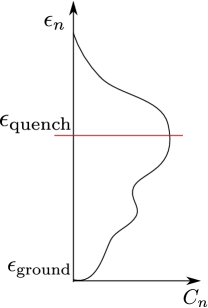
Figure 2: Difference between quench dynamics and thermodynamics. After a quench, the system probes high energy states and does not necessarily relax to the ground state. In thermodynamics, we minimize the energy (or free energy) of a system and probe the region near the ground state.

In the experiments that we seek to describe, a system of $N$ bosons is initially confined to a region of space of size $L$ and then allowed to evolve on the infinite line while interacting with short range interactions. It is important to first understand the time-scales of the phenomena that we are studying. There are two main types of time scales here. One is determined by the initial condition (spatial extent, overlap of nearby wave-functions), and the other by the parameters of the quenched system (mass, interaction strength).

For an extended system where we start with a locally uniform density (see Fig. 1$a$), we expect the dynamics to be in the constant density regime as long as $t\ll\frac{L}{v}$, $v$ being the characteristic velocity of propagation. Although the low energy thermodynamics of a constant density Bose gas can be described by a Luttinger liquid Giamarchi (2004), we expect the collective excitations of the quenched system to behave as a highly excited Liquid since the initial state is far from the ground state. It is also possible that depending on the energy density $\epsilon_{\text{quench}}/L$, the Luttinger liquid description may break down altogether.

The other time scale that enters the description of nonequilibrium dynamics is the interaction time scale, $\tau$, a measure of the time it takes the interactions to develop fully: $\tau\sim\frac{1}{c^{2}}$ for the Lieb-Liniger model . Assuming $L$ is large enough so that $\tau\ll\frac{L}{v}$, we expect a fully interacting regime to be operative at times beyond the interactions scale until $t\gg\frac{L}{v}$ and the density of the system can no longer be considered constant, diminishing with time as the system expands. In the Lieb-Liniger model, this leads to an effective increase in the coupling constant which manifests itself as fermionization for repulsive interaction and bound-state correlations in the case of attractive interactions. Thus the main operation of the interaction occurs in the time range $\tau\lesssim t\lesssim\frac{L}{v}$, over which the wave function rearranges and after which the system is dilute and freely expands. In this low density limit, we cannot make contact with thermodynamic ensembles, in particular, the Generalized Gibbs ensemble Rigol et al. (2007); Calabrese and Cardy (2007); Caux and Essler (2013); Caux and Konik (2012). For the case $L=\infty$, free expansion is not present. Figure 3 summarizes the different time-scales involved in a dynamical situation.

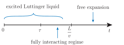
Figure 3: Time scales involved in quench dynamics. $\tau$ is an intrinsic time scale that depends on the interaction strength. $L/v$ is a characteristic time at which the system sees the finite extent.

We shall also consider initial conditions where the bosons are “condensed in space”, occupying the same single particle state characterized by some scale $\sigma$ (see Fig. 1$b$). In this case the short time dynamics is not present, the time scales at which we can measure the system are typically much larger than $\frac{\sigma}{N}$ and we expect the dynamics to be in the strongly interacting and expanding regime.

I.2 Quench dynamics and the Bethe Ansatz

To carry out the computation of the quench dynamics we need to know the eigenstates of the propagating Hamiltonian. The Bethe Ansatz approach is helpful in this respect as it provides us with the eigenstates of a large class of interacting one dimensional Hamiltonians. Many of the Hamiltonians that can be thus be solved are of fundamental importance in condensed matter physics and have been proposed to study various experimental situations. A partial list includes the Heisenberg chain (magnetism), the Hubbard model (strong-correlations), the Lieb-Liniger model (cold atoms in optical traps), the Kondo model, and the Anderson model (impurities in metals, quantum dots) Bethe (1931); Lieb and Wu (1968); Lieb and Liniger (1963); Andrei et al. (1983); Andrei (1995); Tsvelick and Wiegmann (1983). For a Hamiltonian to possess eigenstates that are given in the form of a Bethe Ansatz it must have the property that multi-particle interactions can be consistently factorized into series of two particle interactions, all of them being equivalent.

While originally formulated to understand the Heisenberg chain Bethe (1931), the technology has been studied extensively and recast into a more sophisticated algebraic formulation Sklyanin et al. (1979); Korepin et al. (1997). The usual focus of the Bethe Ansatz approach has been on the thermodynamic properties of the system: determining the spectrum, the free energy, and susceptibilities. Also, considerable efforts were made to compute correlation functions Thacker (1981); Korepin et al. (1997). In particular, the Algebraic Bethe Ansatz has been used in conjunction with numerical methods to calculate so-called form factors which allows access to the dynamical structure functions Mossel and Caux (2012); Calabrese and Caux (2007); Gritsev et al. (2010).

Using the Bethe Ansatz to extract dynamics one encounters a triply complicated problem — the first being to obtain the full spectrum of the Hamiltonian, the second to calculate overlaps, and the third to carry out the sum, which in some cases involves sums over large sets of different “configurations” of states. The overlaps are particularly difficult to evaluate due to the complicated nature of the Bethe eigenstates and their normalization. The problem is more pronounced in the far from equilibrium case of a quench when the state we start with suddenly finds itself far away from the eigenstates of the new Hamiltonian [see eq. (I.2)], and all the eigenstates have non-trivial weights in the time-evolution. In all but the simplest cases, the problem is non-perturbative and the existing analytical techniques are not suited for a direct application to such a situation.

Often quench calculations are carried out in finite volume and the infinite volume limit is taken at the end of the calculation. This may be necessary for thermodynamic calculations, as noted, but not for quench dynamics (see sec. I.1). We shall instead carry out the quench directly in the infinite volume limit in which case the Yudson representation allows us to carry out the calculations in an efficient way, doing away with some of the difficulties mentioned above by not requiring any information about the spectrum, and by using integration as opposed to discrete summation.

More explicitly, the Schrodinger equation for $N$ bosons $H\lvert\vec{\lambda}\rangle=\epsilon(\vec{\lambda})\lvert\vec{\lambda}\rangle$ is satisfied for any value of the momenta $\{\lambda_{j},j=1,\cdots,N\}$ if no boundary conditions are imposed. The initial state can then be written as $\lvert\Psi_{0}\rangle=\int d^{N}\lambda\;C_{\vec{\lambda}}\;\lvert\vec{\lambda}\rangle$, with the integration over $\vec{\lambda}$ replacing the summation. This is akin to summing over an over-complete basis, the relevant elements in the sum being automatically picked up by the overlap with the physical initial state.

It is important to note, however, that while the spectrum of an infinite system is continuous, it can still be very complicated. This is indeed the case with several integrable models, including the Lieb-Liniger model, where the analytic structure of the $S$-matrix (the momentum dependent phase picked up when two particles cross) may permit momenta in the form of complex-conjugate pairs signifying bound states. In the formalism we employ, such states are taken into account by appropriately choosing the contours of integration in the complex plane. This procedure is described in detail.

The remainder of this article is organized as follows. In section II, we briefly discuss experiments with cold atoms. In sections III and IV we will describe the Lieb-Liniger model and Yudson representation for this model, and show how we can use it to calculate the time evolution of an arbitrary initial state. Section V studies the two particle case in detail. We then go on to calculate the evolution of the noise correlations for both the repulsive and the attractive gas at long times in sec. VI. We conclude with a conjecture about the nature of equilibration and thermalization and end with a description of ongoing work and future directions in sec. VII. Appendix A discusses a quench in the Bose-Hubbard model, and why the sign of the interaction doesn’t affect the quench dynamics.

II Experiments with cold atoms

The experimental arena to which our calculations apply are ultracold atomic gases in laser traps, which have become a powerful system for exploring nonequilibrium phenomena Bloch et al. (2008); Cazalilla et al. (2011). The systems are formed by trapping a gas of atoms using standing light waves made by lasers. The gases are cooled evaporatively and are well isolated from any thermal baths making them ideal for studying relaxation and thermalization in isolated quantum systems. The interactions between the particles, the potentials, and their statistics can be controlled by the use of external magnetic and electric fields, tuning the optical lattice, and loading different atoms into the traps. Systems with mobile impurities can also be studied by loading two or more different species of atoms into the lattices. Lattices can be three dimensional or can be made quasi-1$d$ or 2$d$ by using confining potentials. The typical relaxation and evaporation time scales in these systems are in the milliseconds. This makes measurement easier than in solid state systems. It also allows for sudden quenches. Disorder is also largely absent, unless introduced.

Tuning the parameters allows the study of superfluid behavior, Mott insulators, spin chains and so on. Such a gas trapped by lasers and cooled to nano-Kelvin temperatures can be quenched by suddenly changing the interaction between the molecules and the external trapping potential. Evolution can be globally observed by imaging the gas, and the time evolution of densities and correlation functions can be obtained from these images Bloch et al. (2008); Görlitz et al. (2001); Kinoshita et al. (2006); Moritz et al. (2003).

In one dimension, which is of particular interested to us, the typical models that are used to study these systems are the Bose-Hubbard model, the XXZ model, the Sine-Gordon model and the Lieb-Liniger model. Each of these models studies a different regime of the gas. The Bose-Hubbard model is optimal for atoms hopping on a one dimensional lattice. A particular limit of the Bose-Hubbard model can be mapped to the XXZ spin chain Barmettler et al. (2010) which is integrable. The continuum gas is captured by the Lieb-Liniger model.

In this article, we will study the long time dynamics of the Lieb-Liniger model, also an integrable model as mentioned. In this context, it is an important question as to how “integrable” a particular experimental realization is. Often the experimental setup maintains an external trapping potential and including such a potential in an integrable Hamiltonian may render the system non-integrable. Experimentally, such potentials need to be eliminated to the extent possible. This can be partially achieved by using blue/red detuned lasers to create a flat potential well. As has been shown in Ref. Kinoshita et al., 2006, the dynamics in a particular experiment very closely resembles what we expect from an integrable model, and it is believed that we can indeed create integrable systems to a close approximation. This also opens up the question of how far from integrability do we need to be in order to see the effects of integrability breaking. We discuss this point in some detail in the conclusions.

III The Lieb-Liniger model

Bosons in one dimensional traps interact via short range potentials, which can be well approximated by a $\delta$-function interaction. This model was solved in 1963 by Lieb and Liniger Lieb and Liniger (1963) who originally introduced it to overcome shortcomings of other models and approaches for understanding quantum gases and liquids, and to provide a rigorous result to test perturbation theory against. In particular, they sought to improve upon Girardeau’s hard-core boson model Girardeau (1960) by providing a tunable parameter and better model a low density gas, perhaps extensible to higher dimensions. The Schrödinger equation for the model is also commonly known as the Non-linear Schrödinger equation and has been extensively studied both classically and quantum mechanically.

The Hamiltonian is given by

$$H=\int_{x}[\partial b^{\dagger}(x)\partial b(x)+c\,b^{\dagger}(x)b(x)b^{\dagger}(x)b(x)],$$ (III.1)

where $b$ is a bosonic field and $c$ is the interaction strength. The mass has been set to 1/2. The action for the model $\sim\int_{x,t}[\partial_{t}-\partial_{x}^{2}]$. Time therefore has the dimension of (length)². The coupling constant $c$ has the dimensions of length.

The model is integrable and the eigenstates take the Bethe Ansatz form,

$$\lvert\vec{\lambda}\rangle=N(\vec{\lambda})\int_{x}\prod_{i<j}Z_{ij}^{x}(\lambda_{i}-\lambda_{j})\prod_{j}e^{i\lambda_{j}x_{j}}b^{\dagger}(x_{j})\lvert 0\rangle,$$ (III.2)

where $N(\lambda)$ is a normalization factor determined by a particular solution, and

$$Z^{x}_{ij}(z)=\frac{z-ic\operatorname{sgn}(x_{i}-x_{j})}{z-ic}$$ (III.3)

incorporates the two particle $S$-matrix, $S_{ij}=\frac{\lambda_{i}-\lambda_{j}+ic}{\lambda_{i}-\lambda_{j}-ic}$ occurring when two bosons cross. The above state satisfies

$$H\lvert\vec{\lambda}\rangle=\sum_{j}\lambda_{j}^{2}\,\,\lvert\vec{\lambda}\rangle$$ (III.4)

for any value of the momenta $\vec{\lambda}$, which, depending on the sign of $c$, may be pure real or form complex pairs. In our work, we study the evolution dynamics of the model on the infinite line and need not solve for explicit distributions of the $\vec{\lambda}$ that characterize the low lying energy eigenstates, as discussed in section I.1.

IV Yudson representation

In 1985, V. I. Yudson presented a new approach to time evolve the Dicke model (a model for superradiance in quantum optics Dicke (1954)) considered on an infinite line Yudson (1985). The dynamics in certain cases was extracted in closed form with much less work than previously required, and in some cases where it was even impossible with earlier methods. The core of the method is to bypass the laborious sum over momenta using an appropriately chosen set of contours and integrating over momentum variables in the complex plane. It is applicable in its original form to models with a particular pole structure in the two particle $S$-matrix, and a linear spectrum. We generalize the approach to the case of the quadratic spectrum and apply it to the study of quantum quenches.

As discussed earlier, in order to carry out the quench of a system given at $t=0$ in a state $|\Psi_{0}\rangle$ one naturally proceeds by introducing a “unity” in terms of a complete set of eigenstates and then apply the evolution operator–

$$\begin{split}\lvert\Psi_{0},t\rangle=e^{-iHt}\sum_{\{\lambda\}}\lvert\vec{\lambda}\rangle\langle\vec{\lambda}|\Psi_{0}\rangle=\sum_{\{\lambda\}}e^{-i\epsilon(\vec{\lambda})t}\lvert\vec{\lambda}\rangle\langle\vec{\lambda}\rvert\Psi_{0}\rangle\end{split}$$ (IV.1)

The Yudson representation overcomes the difficulties in carrying out this sum by using an integral representation for the complete basis directly in the infinite volume limit.

In the following two sections, we will discuss the representation for the repulsive and attractive models. Each will require a separate set of contours of integrations in order for the representation to be valid. We will notice that in the repulsive case, it is sufficient to integrate over the real line. The attractive case will require the use of contours separated out in the imaginary direction (to be qualified below) consistent with the fact that the spectrum consists of “strings” with momenta taking values as complex conjugate pairs Lieb and Liniger (1963).

IV.1 Repulsive case

We begin by discussing the repulsive case, $c>0$. For this case, a similar approach has been independently developed in Ref. Tracy and Widom, 2008 and has been used by Lamacraft Lamacraft (2011) to calculate noise correlations in the repulsive model. We will start with a generic initial state given by

$$\lvert\Psi_{0}\rangle=\int_{\vec{x}}\Phi_{s}(\vec{x})\prod_{j}b^{{\dagger}}(x_{j})\lvert 0\rangle.$$ (IV.2)

with $\Phi_{s}$ symmetrized. Using the symmetry of the bosonic operators, we can rewrite this state in terms of N-boson coordinate basis states,

$$\lvert\Psi_{0}\rangle=N!\int_{\vec{x}}\Phi_{s}(\vec{x})\lvert\vec{x}\rangle$$ (IV.3)

where,

$$\lvert\vec{x}\rangle=\theta(\vec{x})\prod_{j}b^{\dagger}(x_{j})\lvert 0\rangle.$$ (IV.4)

with $\theta(\vec{x})=\theta(x_{1}>x_{2}>\cdots>x_{N})$. It suffices therefore to show that we can express any coordinate basis state as an integral over the Bethe Ansatz eigenstates

$$\lvert\vec{x}\rangle=\theta(\vec{x})\int_{\gamma}\prod_{j}\frac{\mathrm{d}\lambda_{j}}{2\pi}A(\vec{\lambda},\vec{x})\lvert\vec{\lambda}\rangle$$ (IV.5)

with appropriately chosen contours of integration $\{\gamma_{j}\}$ and $A(\lambda,\vec{x})$, which plays a role similar to the overlap of the eigenstates and the initial state.

We claim that in the repulsive case equation (IV.5) is realized with

$$A(\vec{\lambda},\vec{x})=\prod_{j}e^{-i\lambda_{j}x_{j}}.$$ (IV.6)

and the contours $\gamma_{j}$ running along the real axis from minus to plus infinity. In other words eqn. (IV.5) takes the form,

$$\lvert\vec{x}\rangle=\theta(\vec{x})\int_{\vec{y}}\int\prod_{j}\frac{{\rm d}\lambda_{j}}{2\pi}\>\prod_{i<j}Z^{y}_{ij}(\lambda_{i}-\lambda_{j})\\ \times\prod_{j}e^{i\lambda_{j}(y_{j}-x_{j})}b^{\dagger}(y_{j})\lvert 0\rangle.$$ (IV.7)

Equivalently, we claim that the $\lambda$ integration above produces $\prod_{j}\delta(y_{j}-x_{j})$.

We shall prove this in two stages. Consider first $y_{N}>x_{N}$. To carry out the integral using the residue theorem, we have to close the integration contour in $\lambda_{N}$ in the upper half plane. The poles in $\lambda_{N}$ are at $\lambda_{j}-ic$, $j<N$. These are all below $\gamma_{N}$ and so the result is zero. This implies that any non-zero contribution comes from $y_{N}\leq x_{N}$. Let us now consider $y_{N-1}>x_{N-1}$. The only pole above the contour is $\lambda_{N-1}^{*}=\lambda_{N}+ic$. However, we also have, $y_{N-1}>x_{N-1}>x_{N}\geq y_{N}\implies y_{N-1}>y_{N}$. This causes the only contributing pole to get canceled. The integral is again zero unless $y_{N-1}\leq x_{N-1}$. We can proceed is this fashion for the remaining variables thus showing that the integral is non-zero only for $y_{j}\leq x_{j}$.

Now consider $y_{1}<x_{1}$. We have to close the contour for $\lambda_{1}$ below. There are no poles in that region, and the residue is zero. Thus the integral is non-zero for only $y_{1}=x_{1}$. Consider $y_{2}<x_{2}$. The only pole below, at $\lambda_{2}^{*}=\lambda_{1}-ic$ is canceled as before since we have $y_{2}<x_{2}<x_{1}=y_{1}$. Again we get that the integral is only non-zero for $y_{2}=x_{2}$. Carrying this on, we end up with

$$\theta(\vec{x})\int_{\vec{y}}\prod_{j}\delta(y_{j}-x_{j})b^{\dagger}(y_{j})\lvert 0\rangle=\lvert\vec{x}\rangle.$$ (IV.8)

In order to time evolve this state, we can act on it with the unitary time evolution operator. Since the integrals are well-defined we can move the operator inside the integral signs to obtain,

$$\lvert\vec{x},t\rangle=\theta(\vec{x})\int\prod_{j}\frac{{\rm d}\lambda_{j}}{2\pi}\>e^{-i\epsilon(\vec{\lambda})t}A(\vec{\lambda},\vec{x})\lvert\vec{\lambda}\rangle.$$ (IV.9)

IV.2 Attractive case

We now consider an attractive interaction, $c<0$. As mentioned earlier, this changes the spectrum of the Hamiltonian, allowing complex, so-called string solutions, which in this model, correspond to many-body bound states. In fact, the ground state at $T=0$ consists of one $N$-particle bound state. We will see how the Yudson integral representation takes this into account. Similar properties are seen to emerge in Prolhac and Spohn (2011), where the authors obtain a propagator for the attractive Lieb-Liniger model by analytically continuing the results obtained by Tracy and Widom Tracy and Widom (2008) for the repulsive model.

One will immediately notice from the eigenstates that the pole structure of the $S$-matrix is altered. This change prevents the proof of the previous section from working. In particular, the poles in the variable $\lambda_{N}$ are at $\lambda_{j}+i\lvert c\rvert$ for $j<N$, and the residue of the contour closed in the upper half plane is not zero any more. We need choose a contour to avoid this pole. This can be achieved by separating the contours in the imaginary direction such that adjacent ${\rm Im}[\lambda_{j}-\lambda_{j-1}]>\lvert c\rvert$. At first sight, this seems to pose a problem as the quadratic term in exponent diverges at large positive $\lambda$ and positive imaginary part. There are two ways around this. We can tilt the contours as shown in Fig. 4 so that they lie in the convergent region of the Gaussian integral. The pieces towards the end, that join the real axes though essential for the proof to work at $t=0$, where we evaluate the integrals using the residue theorem, do not contribute at finite time as the integrand vanishes on them as they are taken to infinity.

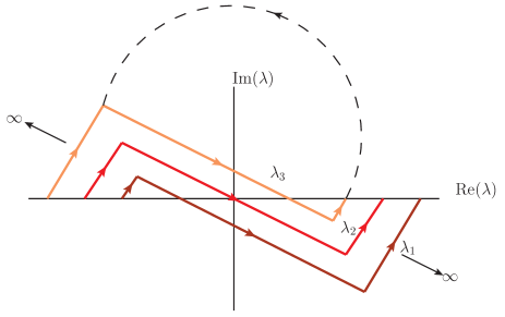
Figure 4: Contours for the $\lambda$ integration. Shown here are three contours, and the closing of the $N$th (here, third) contour as discussed in the proof.

Another more natural means of doing this is to use the finite spatial support of the initial state. The overlaps of the eigenstates with the initial state effectively restricts the support for the $\lambda$ integrals, making them convergent.

The proof of equation (IV.5) now proceeds as in the repulsive case. We start by assuming that $y_{N}>x_{N}$ requiring us to close the contour in $\lambda_{N}$ in the upper half plane. This encloses no poles due to the choice of contours and the integral is zero unless $y_{N}\leq x_{N}$. Now assume $y_{N-1}>x_{N-1}$. Closing the contour above encloses one pole at $\lambda_{N-1}^{*}=\lambda_{N}-i\lvert c\rvert$, however since $y_{N-1}>x_{n-1}>x_{N}\geq y_{N}$, this pole is canceled by the numerator and again we have $y_{N-1}\leq x_{N-1}$. We proceed in this fashion and then backwards to show that the integral is non-zero only when all the poles cancel, giving us $\prod_{j}\delta(y_{j}-x_{j})$, as required.

V Two particle dynamics

We begin with a detailed discussion of the quench dynamics of two bosons. As we saw, it is convenient to express any initial state in terms of an ordered coordinate basis, $\lvert\vec{x}\rangle=\theta(x_{1}>x_{2}>\cdots>x_{N})\prod_{j}b^{\dagger}(x_{j})\lvert 0\rangle$. At finite time, the wave function of bosons initially localized at $x_{1}$ and $x_{2}$ and subsequently evolved by a repulsive Lieb-Liniger Hamiltonian is given by,

$$\begin{split}&\lvert\vec{x},t\rangle_{2}=e^{-iHt}\theta(x_{1}-x_{2})b^{\dagger}(x_{1})b^{\dagger}(x_{2})\lvert 0\rangle\\ &=\int_{y,\lambda}Z^{y}_{12}(\lambda_{1}-\lambda_{2})e^{-i\lambda_{1}^{2}t-i\lambda_{2}^{2}t+i\lambda_{1}(y_{1}-x_{1})+i\lambda_{2}(y_{2}-x_{2})}\\ &\qquad\qquad\times b^{\dagger}(y_{1})b^{\dagger}(y_{2})\lvert 0\rangle\\ &=\int_{y}\frac{e^{i\frac{(y_{1}-x_{1})^{2}}{4t}+i\frac{(y_{2}-x_{2})^{2}}{4t}}}{4\pi it}\\ &\times\Big{[}1-c\sqrt{\pi it}\theta(y_{2}-y_{1})e^{\frac{i}{8t}\alpha^{2}}\operatorname{erfc}\left(\frac{i-1}{4}\frac{i\alpha}{\sqrt{t}}\right)\Big{]}\\ &\times b^{\dagger}(y_{1})b^{\dagger}(y_{2})\lvert 0\rangle.\end{split}$$ (V.1)

where $\alpha=2ct-i(y_{1}-x_{1})-i(y_{2}-x_{2})$. The above expression retains the Bethe form of wave functions defined in different configuration sectors. The only scales in the problem are the interaction strength $c$ and the scale from the initial condition, the separation between the particles at $t=0$.

In order to get physically meaningful results we need to start from a physical initial state. We choose first the state $\lvert\Psi(0)_{\text{latt}}\rangle$ where bosons are trapped in a periodic trap forming initially a lattice-like state (see fig. 1a),

$$\lvert\Psi(0)_{\text{latt}}\rangle=\prod_{j}\left[\frac{1}{(\pi\sigma^{2})^{\frac{1}{4}}}\int_{\vec{x}}e^{-\frac{(x_{j}+(j-1)a)^{2}}{2\sigma^{2}}}b^{\dagger}(x_{j})\right]\lvert 0\rangle.$$ (V.2)

If we assume that the wave functions of neighboring bosons do not overlap significantly, i.e., $e^{-\frac{a^{2}}{\sigma^{2}}}\ll 1$, then the ordering of the initial particles needed for the Yudson representation is induced by the non-overlapping support and it becomes possible to carry out the integral analytically.

We now calculate the evolution of some observable in the state $\lvert\Psi(0)_{\text{latt}}\rangle$. Consider first the evolution of the density $\rho(x)=b^{{\dagger}}(x)b(x)$ at $x=0$. Fig. 5 shows $\langle\Psi_{\text{latt}},t\rvert\rho(0)\lvert\Psi_{\text{latt}},t\rangle$ for repulsive, attractive and non-interacting bosons. No difference is discernible between the three cases. The reason is obvious: the local interaction is operative only when the wave functions of the particles overlap. As we have taken $\sigma\ll a$ this will occur only after a long time when the wave-function is spread out and overlap is negligible.

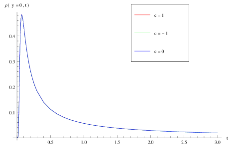
Figure 5: (Color online) $\langle\rho(x=0,t)\rangle$ vs. $t$, after the quench from $\lvert\Psi_{\text{latt}}\rangle$. $\sigma/a\sim 0.1$. The curves appear indistinguishable (i.e. lie on top of each other) since the particles start out with non significant overlap. The interaction effects would show up only when they have propagated long enough to have spread sufficiently to reach a significant overlap, at which time the density is too low.

Consider now an initial state where we set the separation $a$ to zero, starting with maximal initial overlap between the bosons $|\Psi(0)_{\text{cond}}\rangle$. We refer to this state as a condensate (in position-space). Fig. 6 shows the density evolution for attractive, repulsive and no interaction. The decay of the density is slower for attractive model than the for the non-interacting which in turn is slower than for the repulsive model - indeed, unlike before, the interaction is operative from the beginning.

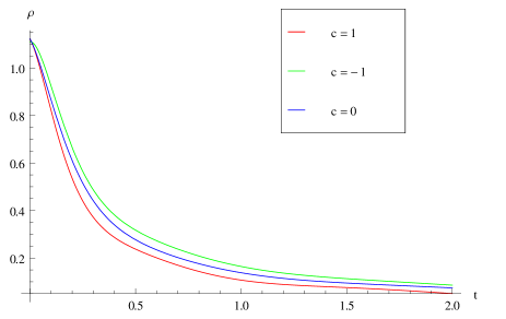
Figure 6: (Color online) $\langle\rho(x=0,t)\rangle$ vs. $t$, after the quench from $\lvert\Psi_{\text{cond}}\rangle$. $\sigma\sim 0.5,\>a=0$. As the bosons overlap interaction effects show up immediately. Lower line: $c=1$, Upper line: $c=-1$, Middle line: $c=0$.

Still, the density does not show much difference between repulsive and attractive interactions in this case. However, a drastic difference will appear when we study the noise correlations $\langle\Psi_{0},t|\rho(x_{1})\rho(x_{2})|\Psi_{0},t\rangle$, as will be shown below.

A comment about the attractive case is in order here. Recall that the contours of integration are separated in the imaginary direction. In order to carry out the integration over $\lambda$, we shift the contour for $\lambda_{2}$ to the real axis, and add the residue of the pole at $\lambda_{2}=\lambda_{1}+i\lvert c\rvert$. The two particle finite time state can be written as

$$\begin{split}&\lvert\vec{x},t\rangle_{2}=\int_{y}\int_{\gamma_{c}}\prod_{i<j=1,2}Z^{y}_{ij}(\lambda_{i}-\lambda_{j})\\ &\qquad\qquad\times\prod_{j=1,2}e^{-i\lambda_{j}^{2}t+i\lambda_{j}(y_{j}-x_{j})}b^{\dagger}(y_{j})\lvert 0\rangle\\ &=\int_{y}\bigg{[}\int_{\gamma_{r}}\prod_{i<j,1}^{2}Z^{y}_{ij}(\lambda_{i}-\lambda_{j})\prod_{j,1}^{2}e^{-i\lambda_{j}^{2}t+i\lambda_{j}(y_{j}-x_{j})}b^{\dagger}(y_{j})\lvert 0\rangle\\ &\qquad+\theta(y_{2}-y_{1})I(\lambda_{2}=\lambda_{1}+i\lvert c\rvert,t)b^{\dagger}(y_{1})b^{\dagger}(y_{2})|0\rangle\bigg{]}\end{split}$$ (V.3)

$\gamma_{c}$ refers to contours that are separated in imaginary direction, $\gamma_{r}$ refers to all $\lambda$ integrated along real axis. $I(\lambda_{2}=\lambda_{1}+i\lvert c\rvert,t)$ is the residue obtained by shifting the $\lambda_{2}$ contour to the real axis from the pole at $\lambda_{2}$ at $\lambda_{1}+i\lvert c\rvert$. This second term corresponds to a two-particle bound state. It is given by

$$\begin{split}&I(\lambda_{2}=\lambda_{1}+i\lvert c\rvert,t)=\\ &-2c\int_{y}\int_{\lambda_{1}}e^{i\lambda_{1}(y_{1}-x_{1})+i(\lambda_{1}+i\lvert c\rvert)(y_{2}-x_{2})-i\lambda_{1}^{2}t-i(\lambda_{1}+i\lvert c\rvert)^{2}t}\\ &=-2c\int_{y}\int_{\lambda_{1}}e^{i\lambda_{1}(y_{1}-x_{1}+y_{2}-x_{2})-\frac{\lvert c\rvert}{2}(y_{2}-y_{1})-\frac{\lvert c\rvert}{2}(x_{1}-x_{2})}\\ &\qquad\qquad\times e^{-i(\lambda_{1}-i\lvert c\rvert/2)^{2}t-i(\lambda_{1}+i\lvert c\rvert/2)^{2}t}\\ &=-c\int_{y}\int_{\lambda_{1}}e^{i\lambda_{1}(y_{1}-x_{1}+y_{2}-x_{2})-\frac{\lvert c\rvert}{2}(x_{1}-x_{2})-\frac{\lvert c\rvert}{2}|y_{2}-y_{1}|}\\ &\qquad\qquad\times e^{-2i\lambda_{1}^{2}t+i\frac{\lvert c\rvert^{2}}{2}t}.\end{split}$$ (V.4)

This contribution corresponds to the particles propagating as a bound state, $e^{-\frac{\lvert c\rvert}{2}|y_{2}-y_{1}|}$, with kinetic energy $E_{k}=2\lambda_{1}^{2}$, and binding energy $E_{b}=-c^{2}/2$. The rest of the expression, $e^{i\lambda_{1}(y_{1}-x_{1}+y_{2}-x_{2})-\frac{\lvert c\rvert}{2}(x_{1}-x_{2})}$, yields the overlap of the bound state with the initial state $|\vec{x}\rangle$. Note that the overlap decays exponentially as the distance $\lvert x_{1}-x_{2}\rvert$ between the initial positions is increased.

Such bound states appear for any number of particles involved. For instance, for three particles, the Yudson representation with complex $\lambda$s automatically produces multiple bound-states coming from the poles, i.e. $I(\lambda_{2}=\lambda_{1}+i\lvert c\rvert)$, $I(\lambda_{3}=\lambda_{1}+i\lvert c\rvert)$, etc. They give rise to two and three particle bound states, the latter being of the form $e^{-\frac{|c|}{2}(|y_{1}-y_{2}|+|y_{1}-y_{3}|+|y_{2}-y_{3}|)}$ with binding energy $E_{b}=-2c^{2}$. It is important to remark that these bound states were not put in by hand, but arise straightforwardly from the contour representation. The binding energy of an $N$-particle bound state thus appearing in the time evolution is $E_{b}=-c^{2}N(N^{2}-1)/12$ as expected from the spectrum of the Hamiltonian Yang (1968).

Finally, we combine the bound state contribution discussed above and the “real axis” term, $\int_{y}\int_{\gamma_{r}}\prod_{i<j,1}^{2}Z^{y}_{ij}(\lambda_{i}-\lambda_{j})\prod_{j,1}^{2}e^{-i\lambda_{j}^{2}t+i\lambda_{j}(y_{j}-x_{j})}b^{\dagger}(y_{j})\lvert 0\rangle$, which corresponds to the non-bound propagating states in (LABEL:eq:att2pint). The resulting wave function is,

$$\begin{split}&\lvert\vec{x},t\rangle_{2}=\int_{y}\frac{e^{i\frac{(y_{1}-x_{1})^{2}}{4t}+i\frac{(y_{2}-x_{2})^{2}}{4t}}}{4\pi it}\\ &\left[1+\lvert c\rvert\sqrt{\pi it}\theta(y_{2}-y_{1})e^{\frac{i}{8t}\tilde{\alpha}^{2}}\operatorname{erfc}\left(\frac{i-1}{4}\frac{i\tilde{\alpha}}{\sqrt{t}}\right)\right]\\ &\qquad\qquad\qquad\times b^{\dagger}(y_{1})b^{\dagger}(y_{2})|0\rangle\end{split}$$ (V.5)

where $\tilde{\alpha}=-2\lvert c\rvert t-i(y_{1}-x_{1})-i(y_{2}-x_{2})$. Surprisingly, the wave function maintains its form and we only need to replace $c\to-c$. This simple result is not valid for more than two particles.

We now compute the noise correlation in the evolving state. We expect the interaction to have a a significant effect as the geometry of the set up measures the interference of “direct” and “crossed” measurements as shown in fig. 7a.

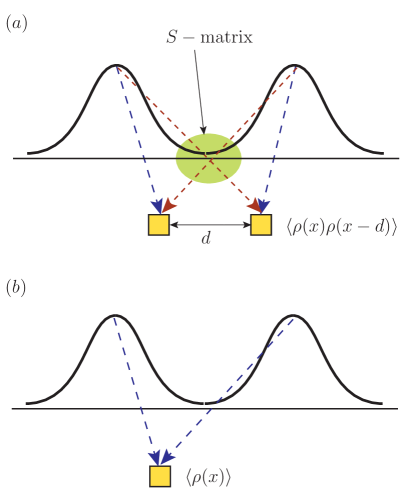
Figure 7: $(a)$ The Hanbury-Brown Twiss effect, where two detectors are used to measure the interference of the direct (big dashes) and the crossed waves (small dashes). The $S$-matrix enters explicitly. $(b)$ The density measurement is not directly sensitive to the $S$-matrix. The thick black line shows the wave-function amplitude, the dotted lines show time propagation.

In contrast, the density measurements do not see the $S$-matrix, as shown in fig. 7$b$.

This is the famous Hanbury-Brown Twiss experiment Hanbury-Brown and Twiss (1956) where for free bosons or fermions, the crossing produces a phase of $\pm 1$ and causes destructive or constructive interference. In our case the set up is generalized to multiple time dependent sources with the phase given by the two particle $S$-matrix capturing the interactions between the particles. In Fig. 8 we present the two point correlation matrix $\langle\rho(x_{1})\rho(x_{2})\rangle$ for the repulsive gas, attractive gas, and the non-interacting gas, shown at different times, starting with the lattice initial state. Figure 9 shows the same for the condensate initial state.

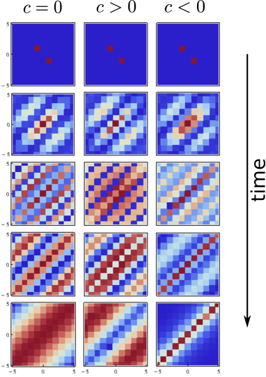
Figure 8: (Color online) Time evolution of density-density correlation matrix ($\langle\rho(x)\rho(y)\rangle$) for the $\lvert\Psi_{\text{latt}}\rangle$ initial state. Blue is zero and red is positive. The repulsive model shows anti-bunching, i.e., fermionization at long times, while the attractive model shows bunching.

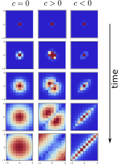
Figure 9: (Color online) Time evolution of density-density correlation matrix ($\langle\rho(x)\rho(y)\rangle$) for the $\lvert\Psi_{\text{cond}}\rangle$ initial state. Blue is zero and red is positive. The repulsive model shows anti-bunching, i.e., fermionization at long times, while the attractive model shows bunching.

In both these, we note that the repulsive gas develops fermionic correlations (i.e., strong anti-bunching), and the attractive gas retains bosonic correlations at long time, showing strong bunching.

It is interesting to compare this result with the time evolution after a quench on the lattice by the Bose-Hubbard model, the lattice counterpart of the Lieb-Liniger model, as we shall see in Appendix A. The results for continuum model differs strongly from those of the lattice model.

We expect the results to be qualitatively similar for higher particle number. In order to go beyond two particles however, the integrations cannot be carried out exactly. However, we can extract the asymptotic behavior of the wavefunction analytically, as we show below.

VI Multiparticle dynamics at long times

In this section, we derive an expression for the multiparticle wavefunction evolution at long times. The number of particles $N$ is kept fixed in the limiting process, hence, as discussed in the introduction we are in the low density limit where interactions are expected to be dominant. The other regime where $N$ is sent to infinity first will be discussed in a separate report. We first deal with the repulsive model, for which no bound states exist and the momentum integrations can be carried out over the real line, and then proceed to the attractive model. In a separate sub-section, we examine the effect of starting with a condensate-like initial state.

VI.1 Repulsive interactions - Asymptotics

From (IV.5) we can see by scaling $\lambda\to\lambda\sqrt{t}$, we get

$$Z^{y}_{ij}(\lambda_{i}-\lambda_{j})\to\operatorname{sgn}(y_{i}-y_{j})+O\left(\frac{1}{\sqrt{t}}\right),$$ (VI.1)

yielding to leading order,

$$\begin{split}&|\Psi_{0},t\rangle\to\int_{x}\int_{y}\int_{\lambda}\,\theta(\vec{x})\Psi_{0}(\vec{x})\\ &\times\prod_{j}\frac{1}{\sqrt{t}}e^{-i\lambda_{j}^{2}+i\lambda_{j}(y_{j}-x_{j})/\sqrt{t}}\prod_{i<j}\operatorname{sgn}(y_{i}-y_{j})b^{\dagger}(y_{j})\lvert 0\rangle\\ &=\int_{x,y,\lambda,k}\,\theta(\vec{x})\Psi_{0}(\vec{x})\prod_{j}e^{-i\lambda_{j}^{2}t+i\lambda_{j}(y_{j}-x_{j})}e^{-ik_{j}y_{j}}c^{{\dagger}}_{k_{j}}\lvert 0\rangle\\ &=\int_{x,k}\,\theta(\vec{x})\Psi_{0}(\vec{x})\prod_{j}e^{-ik_{j}^{2}t-ik_{j}x_{j}}c^{{\dagger}}_{k_{j}}\lvert 0\rangle\\ &=e^{-iH^{f}_{0}t}\int_{x}\mathcal{A}_{x}\theta(\vec{x})\Psi_{0}(\vec{x})\prod_{j}c^{\dagger}(x_{j})\lvert 0\rangle,\end{split}$$

$c^{\dagger}(y)$ being fermionic creation operators replacing the “fermionized” hardcore bosonic operators, $\prod_{j}c^{\dagger}(y_{j})=\prod_{i<j}\operatorname{sgn}(y_{i}-y_{j})b^{\dagger}(y_{j})$. We denote $H^{f}_{0}=\int_{x}\partial c^{\dagger}(x)\partial c(x)$ the free fermionic Hamiltonian and $\mathcal{A}_{y}$ is an anti-symmetrizer acting on the $y$ variables. Thus, the repulsive Bose gas, for any value of $c>0$, is governed in the long time by the $c=\infty$ hard core boson limit (or its fermionic equivalent) Jukić et al. (2008); Girardeau (1960), and the system equilibrates with an asymptotic momentum distribution, $n_{k}=\langle\tilde{\Psi}_{0}|c^{\dagger}_{k}c_{k}|\tilde{\Psi}_{0}\rangle$, determined by the antisymmetric wavefunction $\tilde{\Psi}_{0}(\vec{y})=\mathcal{A}_{y}\theta(\vec{y})\Psi_{0}(\vec{y})$ and the total energy, $E_{\Psi_{0}}=\langle\Psi_{0}\rvert H\lvert\Psi_{0}\rangle$.

We will now derive the corrections to the infinite time limit. At large time, we use the stationary phase approximation to carry out the $\lambda$ integrations. The phase oscillations come primarily from the exponent $e^{-i\lambda_{j}^{2}t+i\lambda_{j}(y_{j}-x_{j})}$. At large $t$ (i.e., $t\gg\frac{1}{c^{2}}$), the oscillations are rapid, and the stationary point is obtained by solving

$$\frac{\operatorname{d}}{\operatorname{d}\lambda_{j}}[-i\lambda_{j}^{2}t+i\lambda_{j}(y_{j}-x_{j})]=0.$$ (VI.2)

Note that typically one would ignore the second term above since it doesn’t oscillate faster with increasing $t$, but here we cannot since the integral over $y$ produces a non-zero contribution for $y\sim t$ at large time. Doing the Gaussian integral around this point (and fixing the $S$-matrix prefactor to its stationary value), we obtain for the repulsive case,

$$\lvert\vec{x},t\rangle\to\int_{y}\prod_{i<j}Z^{y}_{ij}\left(\frac{y_{i}-y_{j}-x_{i}+x_{j}}{2t}\right)\\ \times\prod_{j}\frac{1}{\sqrt{4\pi it}}e^{-i\frac{(y_{j}-x_{j})^{2}}{4t}+i\frac{(y_{j}-x_{j})^{2}}{2t}}b^{\dagger}(y_{j})\lvert 0\rangle.$$ (VI.3)

In the above expression, the wavefunction has support mainly from regions where $y_{j}/t$ is of order one. In an experimental setup, one typically starts with a local finite density gas, i.e., a finite number of particles localized over a finite length. With this condition, at long time, we can neglect $x_{j}/t$ in comparison with $y_{j}/t$, giving

$$\lvert\vec{x},t\rangle\to\int_{y}\prod_{i<j}Z_{ij}(\xi_{i}-\xi_{j})\prod_{j}\frac{1}{\sqrt{4\pi it}}e^{it\xi_{j}^{2}-i\xi_{j}x_{j}}b^{\dagger}(y_{j})\lvert 0\rangle$$ (VI.4)

where $\xi=\frac{y}{2t}$.

We turn now to calculated the asymptotic evolution of some observables. To compute the expectation value of the density we start from the coordinate basis states, $\langle\vec{x^{\prime}},t\rvert\rho(z)\lvert\vec{x},t\rangle$ which we then integrate with the chosen initial state,

$$\langle\vec{x^{\prime}},t\rvert\rho(z)\lvert\vec{x},t\rangle=\sum_{\{P\}}\int_{y}\left(\sum_{j}\delta(y_{j}-z)\right)\\ \times\prod_{i<j}Z_{ij}(\xi_{i}-\xi_{j})Z^{*}_{P_{i}P_{j}}(\xi_{P_{i}}-\xi_{P_{j}})\prod_{j}\frac{1}{4\pi t}e^{-i(\xi_{j}x_{j}-\xi_{P_{j}}x^{\prime}_{j})}$$ (VI.5)

Note that the above product of $S$-matrices is actually independent of the ordering of the $y$. First, only those terms appear in the product for which the permutation $P$ has an inversion. For example, say for three particles, if $P=312$, then the inversions are 13 and 23. It is only these terms which give a non-trivial $S$-matrix contribution. For the non-inverted terms, here 12, we get

$$\frac{\xi_{1}-\xi_{2}-ic\operatorname{sgn}(y_{1}-y_{2})}{\xi_{1}-\xi_{2}-ic}\frac{\xi_{1}-\xi_{2}+ic\operatorname{sgn}(y_{1}-y_{2})}{\xi_{1}-\xi_{2}+ic}$$ (VI.6)

which is always unity irrespective of the ordering of $y_{1},y_{2}$. For a term with an inversion, say 23, we get,

$$\frac{\xi_{2}-\xi_{3}-ic\operatorname{sgn}(y_{2}-y_{3})}{\xi_{2}-\xi_{3}-ic}\frac{\xi_{3}-\xi_{2}+ic\operatorname{sgn}(y_{3}-y_{2})}{\xi_{3}-\xi_{2}+ic}$$ (VI.7)

which is always equal to

$$\frac{\xi_{2}-\xi_{3}+ic}{\xi_{2}-\xi_{3}-ic}\equiv S(\xi_{2}-\xi_{3})$$ (VI.8)

irrespective of the sign of $y_{2}-y_{3}$. This allows us to carry out the integration over the $y_{j}$.

VI.1.1 Lattice initial state

In order to calculate physical observables, we have to choose initial states. We choose two different initial states for the problem, one with $N$ particles distributed with uniform density in a series of harmonic traps given by,

$$\lvert\Psi_{\text{latt}}\rangle=\int_{x}\prod_{j=1}^{N}\frac{1}{(\pi\sigma^{2})^{\frac{1}{4}}}e^{-\frac{(x_{j}+(j-1)a)^{2}}{2\sigma^{2}}}b^{\dagger}(x_{j})\lvert 0\rangle,$$ (VI.9)

such that the overlap between the wave functions of two neighboring particles is negligible. In this particular case, the ordering of the particles is induced by the limited non-overlapping support of the wave function.

In the lattice-like state, the initial wave function starts out with the neighboring particles having negligible overlap. At small time (as seen from (V.1)), the particle repel each other, but they never cross due to the repulsive interaction. So at large time, the interaction does not play a role since the wave functions are sufficiently non-overlapping. It is only the $P=1$ contribution then that survives, and we get for the density

$$\langle\vec{x}^{\prime},t\rvert\rho(z)\lvert\vec{x},t\rangle=\sum_{j}\prod_{k\neq j}\frac{\delta(x_{k}-x_{k}^{\prime})e^{-i\frac{z}{2t}(x_{j}-x_{j}^{\prime})}}{4\pi t}.$$ (VI.10)

We need to integrate the position basis vectors $\lvert\vec{x}\rangle$ over some initial condition. We do this here for the lattice state (VI.9) This gives

$$\langle\Psi_{\text{latt}},t\rvert\rho(z)\lvert\Psi_{\text{latt}},t\rangle=\rho_{\text{latt}}(\xi_{z})=\frac{N\sigma}{2\sqrt{\pi}t}e^{-\frac{\xi_{z}^{2}}{\sigma^{2}}}$$ (VI.11)

Mathematically, any $S$-matrix factor that appears will necessarily have zero contribution from the pole - this is easy to see from the pole structure, and the ordering of the coordinates. In order to get a non-zero result, we need to fix at least two integration variables (i.e., the $y_{j}$). Thus the first non-trivial contribution comes from the two-point correlation function.

We now proceed to calculate the evolution of the noise, i.e., the two body correlation function $\rho_{2}(z,z^{\prime};t)_{\text{latt}}=\langle\Psi_{\text{latt}},t\rvert\rho(z)\rho(z^{\prime})\lvert\Psi_{\text{latt}},t\rangle$. The contributions can be grouped in terms of number of crossings, which corresponds to a grouping in terms of the coefficient $e^{-ca}$ Lamacraft (2011). The leading order term can be explicitly evaluated and we show below which terms contribute. In general we have

$$\rho_{2\text{ latt}}(z,z^{\prime};t)=\sum_{\{P\}}\int_{y}\left(\sum_{j,K}\delta(y_{j}-z)\delta(y_{k}-z^{\prime})\right)\\ \times\prod_{i<j,(ij)\in P}S(\xi_{i}-\xi_{j})\prod_{j}\frac{1}{4\pi t}e^{-i(\xi_{j}x_{j}-\xi_{P_{j}}x^{\prime}_{j})}.$$ (VI.12)

The above shorthand in the $S$-matrix product means that only the $(ij)$ that belong to the inversions in $P$ are included. We will now determine which terms contribute in this sum. First note that for integration over a particular $\xi_{j}$, the residue depends on the sign of $x_{j}-x_{P_{j}}$. Let us consider a specific example. Consider the three particle case with the term $P=321$. All three $S$-matrix factors appear in this term. $\xi_{3}$ has a pole at $\xi_{1}-ic$ and $\xi_{2}-ic$. Thus integrating over $y_{3}$ will give a non-zero residue only if $x_{3}>x_{1}^{\prime}$ which is however not satisfied by the initial conditions we choose. So, everything is zero, unless we do not integrate over $y_{3}$, implying it has to be one of the measured variables. Similarly for $\xi_{1}$, the poles are at $\xi_{2}+ic$ and $\xi_{3}+ic$. In order to get a non-zero residue we need $x_{1}<x_{3}^{\prime}$ which again is not satisfied by the initial conditions. We get a non-zero result if we pin $\xi_{1}$. As for $\xi_{2}$ it has poles both above and below the real line and so this always gives a non-zero contribution irrespective of the sign of $x_{2}-x_{2}^{\prime}$.

One can see that this argument can be extended to the case with more particles. Depending on what coordinates we are measuring at, we’ll get a specific contribution from the sum over permutations. The next simplification comes from not allowing any crossings among the unmeasured coordinates. It can be shown that allowing for these gives us a higher order contribution in $e^{-ca}$. In other words, the leading order contribution comes from terms such as $P=21,32,321,4231,5342,52341,\ldots$. The only exchanges are on the ends. A general term will therefore look like (for $l<k$),

$$\begin{split}&\int_{y}\delta(y_{l}-z)\delta(y_{k}-z^{\prime})\prod_{j\neq\{l,k\}}S(\xi_{i}-\xi_{j})S(\xi_{j}-\xi_{k})\\ &\times\frac{e^{-i\xi_{j}(x_{j}-x_{j}^{\prime})}}{4\pi t}\frac{\xi_{l}-\xi_{k}+ic}{\xi_{l}-\xi_{k}-ic}\frac{e^{-i\xi_{l}(x_{l}-x_{k}^{\prime})-i\xi_{k}(x_{k}-x_{l}^{\prime})}}{(4\pi t)^{2}}\end{split}$$ (VI.13)

We have to sum over $l,k$, which will automatically sum over the number of intermediate $j$’s appearing. We’ll integrate the above general term, since the $y_{j}$ integrals factor anyway. This gives

$$\prod_{i\neq k,l,j}\delta(x_{i}-x^{\prime}_{i})S(\xi_{l}-\xi_{k})\frac{e^{-i\xi_{l}(x_{l}-x^{\prime}_{k})-i\xi_{k}(x_{k}-x^{\prime}_{l})}}{(4\pi t)^{2}}\\ \times\prod_{j}\bigg{[}\delta(x_{j}-x^{\prime}_{j})-S(\xi_{l}-\xi_{k}-ic)\\ \times\bigg{\{}\theta(x_{j}>x^{\prime}_{j})e^{-i(\xi_{l}-ic)(x_{j}-x^{\prime}_{j})}+\\ +\theta(x_{j}<x^{\prime}_{j})e^{-i(\xi_{k}+ic)(x_{j}-x^{\prime}_{j})}\bigg{\}}\bigg{]}$$ (VI.14)

We can sum the different contributions now. Note that the number of terms appearing the product over $j$ is given by $k-l-1$. So for a given $l$, we have to sum over all the $k$. Using a shorthand notation, the sum can be written as (note that it is understood that $y_{l}$ and $y_{k}$ are integrated over using the delta functions. We retain the indices to keep track of the terms. We actually have $\xi_{l}=2zt$ and $\xi_{k}=2z^{\prime}t$.

$$\sum_{l,k}\prod_{i<l,i>k}\delta_{i}f_{lk}\prod_{j=l+1}^{k-1}g_{jlk}$$ (VI.15)

In order to proceed with the summation, we have to integrate over the $x$. We use the initial conditions described by (VI.9), i.e., the lattice-like state. We’ll do it term by term.

$$\int_{x_{i},x^{\prime}_{i}}\delta(x_{i}-x^{\prime}_{i})\frac{e^{-\frac{(x_{i}+(i-1)a)^{2}}{2\sigma^{2}}-\frac{(x^{\prime}_{i}+(i-1)a)^{2}}{2\sigma^{2}}}}{\sqrt{\pi\sigma^{2}}}=1$$ (VI.16)

$$\int_{x_{l},x^{\prime}_{k},x_{k},x^{\prime}_{l}}f_{lk}\frac{e^{-\sum_{l,k,l^{\prime},k^{\prime}}\frac{(x_{l}+(l-1)a)^{2}}{2\sigma^{2}}}}{\pi\sigma^{2}}\\ =\frac{\sigma^{2}}{4\pi t^{2}}S(\xi_{l}-\xi_{k})e^{-(\xi_{l}^{2}+\xi_{k}^{2})\sigma^{2}}e^{ia(k-l)(\xi_{k}-\xi_{l})}$$ (VI.17)

$$\int_{x_{j},x^{\prime}_{j}}g_{jlk}\frac{e^{-\frac{(x_{j}+(j-1)a)^{2}}{2\sigma^{2}}-\frac{(x^{\prime}_{j}+(j-1)a)^{2}}{2\sigma^{2}}}}{\pi\sigma^{2}}=1-2c\sqrt{\pi}\sigma\\ \times S(\xi_{l}-\xi_{k}-ic)\Big{[}e^{(c+i\xi_{l})^{2}\sigma^{2}}\operatorname{erfc}\{(c+i\xi_{l})\sigma\}+\\ +e^{(c-i\xi_{k})^{2}\sigma^{2}}\operatorname{erfc}\{(c-i\xi_{k})\sigma\}\Big{]}$$ (VI.18)

Note that last expression has no $j$ dependence. So, the sum over the product over $j$ is just a geometric series. Recall that $\xi_{l}$ and $\xi_{k}$ are fixed at $z$ and $z^{\prime}$ respectively. This series can be summed. Note that the number of terms in the product is equal to the $k-l$, and summing over them is effectively summing over $k$. The previous term therefore needs to be taken into account. Writing $\xi_{l}=\xi_{z}$ and $\xi_{k}=\xi_{z^{\prime}}$, we can write the sum as

$$\frac{\sigma^{2}}{4\pi t^{2}}S(\xi_{z}-\xi_{z^{\prime}})e^{-(\xi_{x}^{2}+\xi_{z^{\prime}}^{2})\sigma^{2}}\sum_{l<k}e^{ia(k-l)(\xi_{z}-\xi_{z^{\prime}})}g_{zz^{\prime}}^{k-l-1}$$ (VI.19)

where

$$g_{zz^{\prime}}=1-2c\sqrt{\pi}\sigma S(\xi_{z}-\xi_{z^{\prime}}-ic)\\ \times\Big{[}e^{(c+i\xi_{z})^{2}\sigma^{2}}\operatorname{erfc}\{(c+i\xi_{z})\sigma\}+\\ +e^{(c-i\xi_{z^{\prime}})^{2}\sigma^{2}}\operatorname{erfc}\{(c-i\xi_{z^{\prime}})\sigma\}\Big{]}$$ (VI.20)

Finally, we have to account for the $k>l$ case which is equivalent to setting $\xi_{l}=\xi_{z^{\prime}}$ and $\xi_{l}=\xi_{z}$. Doing this is further equivalent to adding the complex conjugate. We also have to take into account the term with no permutations. So, finally we have,

$$\rho_{2\text{ latt}}(z,z^{\prime})=\frac{N^{2}\sigma^{2}}{4\pi t^{2}}e^{-(\xi_{x}^{2}+\xi_{z^{\prime}}^{2})\sigma^{2}}\bigg{[}1+\frac{2}{N^{2}}\mathrm{Re}S(\xi_{z}-\xi_{z^{\prime}})\\ \times e^{ia(z-z^{\prime})}\frac{N(1-e^{ia(z-z^{\prime})}g)+e^{iaN(z-z^{\prime})}g_{zz^{\prime}}^{N}-1}{[1-g_{zz^{\prime}}e^{ia(z-z^{\prime})}]^{2}}\bigg{]}$$ (VI.21)

To compare with the Hanbury-Brown Twiss result, we calculate the normalized spatial noise correlations, given by $C_{2}(z,z^{\prime})\equiv\frac{\rho_{2}(z,z^{\prime})}{\rho(z)\rho(z^{\prime})}-1\equiv C_{2}(z,z^{\prime})$. In the non-interacting case, i.e., $c=0$, $S(\xi)=1$ and $g_{zz^{\prime}}=0$ and we recover the HBT result for $N=2$,

$$C_{2}^{0}(\xi_{z},\xi_{z^{\prime}})=\frac{1}{2}\cos(a(\xi_{z}-\xi_{z}^{\prime}))$$ (VI.22)

One can also check that the limit of $c\to\infty$ gives the expected answer for free fermions, namely,

$$C_{2}^{\infty}(\xi_{z},\xi_{z^{\prime}})=-\frac{1}{2}\cos(a(\xi_{z}-\xi_{z}^{\prime}))$$ (VI.23)

At finite $c$ we can see a sharp fermionic character appear that broadens with increasing $c$ as shown in Fig. 10.

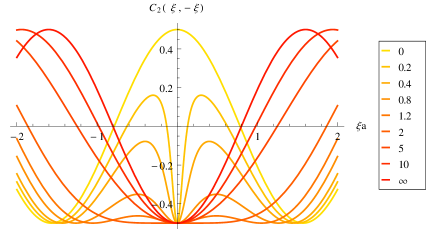
Figure 10: (Color online) Normalized noise correlation function $C_{2}(\xi,-\xi)$. Fermionic correlations develop on a time scale $\tau\sim c^{-2}$, so that for any $c$ we get a sharp fermionic peak near $\xi=0$, i.e., at large time. The key shows values of $ca$ (from Ref. Iyer and Andrei, 2012).

The large time behavior is captured in a small window around $\xi=0$. One can see that at any finite $c$, the region near zero develops a strong fermionic character, thus indicating that irrespective of the value of the coupling that we start with, the model flows towards an infinitely repulsive model at large time, that can be described in terms of free fermions. We also obtained this result “at” $t=\infty$ at the beginning of this section.

For higher particle number, we see “interference fringes” corresponding to the number of particles, that get narrower and more numerous with an increase, memory of the initial lattice state. However, the asymptotic fermionic character does not disappear. Figures 11 and 12 show the noise correlation function for five and ten particles respectively. The large peaks are interspersed by smaller peaks and so on. This reflects the character of the initial state.

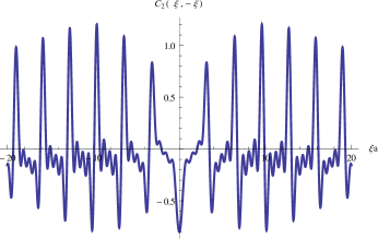
Figure 11: Normalized noise correlation function for five particles released for a Mott-like state for $c>0$ (from Ref. Iyer and Andrei, 2012)

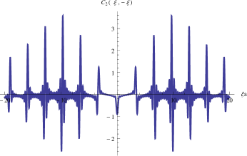
Figure 12: Normalized noise correlation function for ten particles released for a Mott-like state for $c>0$.

VI.1.2 Quenching from a bound state

In this brief section our initial state is the ground state of the attractive Lieb-Liniger Hamiltonian (with interaction strength $-c_{0}<0$. For two bosons, this take the form Lieb and Liniger (1963),

$$\lvert\Psi_{\text{bound}}\rangle=\int_{\vec{x}}e^{-c_{0}\lvert x_{1}-x_{2}\rvert-\frac{x_{1}^{2}}{2\sigma^{2}}-\frac{x_{2}^{2}}{2\sigma^{2}}}b^{{\dagger}}(x_{1})b^{{\dagger}}(x_{2})\lvert 0\rangle,$$ (VI.24)

and we quench it with a repulsive Hamiltonian.The long time noise correlations are displayed in Fig. 13. We see that while the initial state correlations are preserved over most of the evolution, in the asymptotic long time limit the characteristic fermionic dip.

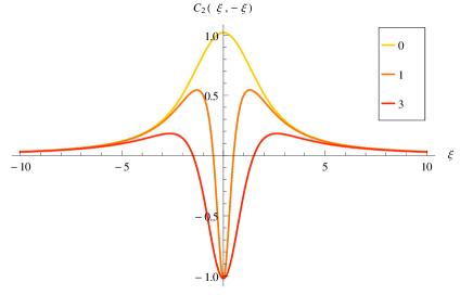
Figure 13: (Color online) Normalized noise correlation function for two particle quenched from a bound state into the repulsive regime. The legend indicates the values of $c$ that the state is quenched into. We start with $c_{0}\sigma^{2}=3,\;\sigma=1$, $c_{0}$ being the interaction strength of the initial state Hamiltonian. Again, we see the fermionic dip, but the rest of the structure is determined by the initial state.

We expect similar effects for any number of bosons.

VI.2 Attractive interactions

For the attractive case, since the contours of integration are spread out in the imaginary direction, we have the contributions from the poles in addition to the stationary phase contributions at large time. The stationary phase contribution is picked up on the real line, but as we move the contour, it stays pinned above the poles and we need to include the residue obtained from going around them, leading to sum over several terms.Fig. 14 shows an example of how this works.

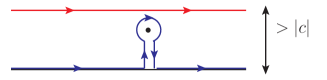
Figure 14: (Color online) Contribution from stationary phase and pole at large time in the attractive model. The blue (lower) contour represents the shifted contour.

In Ref. Iyer and Andrei, 2012, a formula was provided for the asymptotic state. Here we give a more careful treatment by taking into account that the fixed point of the approximation moves for terms that come from a pole of the $S$-matrix. It is therefore necessary to first shift the contours of integration, and then carry out the integral at long time. We carry this out below.

Shifting a contour over a pole leads to an additional term from the residue:

$$\int_{\gamma_{2}}\frac{{\rm d}\lambda_{2}}{2\pi}\to\int_{\gamma^{\rm R}_{2}}\frac{{\rm d}\lambda_{2}}{2\pi}-i\mathcal{R}(\lambda_{2}\to\lambda_{1}+i\lvert c\rvert)$$ (VI.25)

where $\mathcal{R}(x)$ indicates that we evaluate the residue given by the pole $x$. $\gamma_{j}$ indicates the original contour of integration and $\gamma_{j}^{\rm R}$ indicates that integration is carried out over the real axis. Proceeding with the other variables we end up with

$$\int_{\gamma_{1},\gamma_{2},\cdots,\gamma_{N}}\to\int_{\gamma^{\rm R}_{1}}\left[\int_{\gamma^{\rm R}_{2}}+i\mathcal{R}(\lambda_{2}\to\lambda_{1}+i\lvert c\rvert)\right]\\ \times\left[\int_{\gamma^{\rm R}_{3}}+i\mathcal{R}(\lambda_{3}\to\lambda_{1}+i\lvert c\rvert)+i\mathcal{R}(\lambda_{3}\to\lambda_{2}+i\lvert c\rvert)\right]\cdots\\ \times\Big{[}\int_{\gamma^{\rm R}_{N}}+i\mathcal{R}(\lambda_{N}\to\lambda_{1}+i\lvert c\rvert)+i\mathcal{R}(\lambda_{N}\to\lambda_{2}+i\lvert c\rvert)+\\ +\cdots+i\mathcal{R}(\lambda_{N}\to\lambda_{N-1}+i\lvert c\rvert)\Big{]}$$ (VI.26)

The integrals can now be evaluated using the stationary phase approximation. The correction produced by the above procedure does not affect the qualitative features observed in Ref. Iyer and Andrei, 2012.

VI.2.1 Lattice initial state

We now calculate the evolution of the density and the two body correlation function in order to compare with the repulsive case. We will first study the two particle case. Although we have a finite time expression for this case from which we can directly take a long time limit, we will study the asymptotics using the above scheme for an $N$-particle state, since we have an analytical expression to go with. We get two terms, the first being the stationary phase contribution, and is just like the repulsive case with $c\to-c$. The second is the contribution from the pole. It contains the bound state contribution which brings about another interesting feature of the attractive case. While the asymptotic dynamics of the repulsive model is solely dictated by the new variables $\xi_{j}\equiv\frac{y_{j}}{2t}$, and all the time dependence of the wave function enters through this “velocity” variable, this is not the case in the attractive model. While it is true that the system is naturally described in terms of $\xi$ variables, there still exists non-trivial time dependence.

First, we integrate out the $x$ dependence assuming an initial lattice-like state. This gives,

$$\lvert\Psi_{\text{latt}}(t)\rangle=\int_{y}\sum_{\xi_{j}^{*}=\xi_{j},\xi_{i}^{*}+ic,i<j}\prod_{i<j}S_{ij}(\xi_{i}^{*}-\xi_{j}^{*})\prod_{j}\frac{(4\pi\sigma^{2})^{\frac{1}{4}}}{\sqrt{4\pi it}}\\ \times e^{-(\sigma^{2}/2+it)(\xi_{j}^{*})^{2}+i\xi_{j}^{*}(2t\xi_{j}+a(j-1))}b^{\dagger}(y_{j})\lvert 0\rangle.$$ (VI.27)

Defining $\phi(\xi,t)$ from $\lvert\Psi_{\text{latt}}(t)\rangle=\int_{y}\phi(\xi,t)\prod_{j}b^{\dagger}(y_{j})\lvert 0\rangle$, we have for the density evolution under attractive interactions, $c<0$,

$$\rho_{\text{latt}}^{-}(z;t)=\sum_{\{P\},j}\int_{y}\delta(y_{j}-z)\phi^{*}(\xi_{P},t)\phi(\xi,t)$$ (VI.28)

We can show numerically (the expressions are a bit unwieldy to write here), that asymptotically, the density shows the same Gaussian profile that we expect from a uniformly diffusing gas, namely, $e^{-\xi^{2}\sigma^{2}}$.

With this, we can proceed to compute the noise correlation function. The two particle case is easy, as there are no more integrations to carry out. We get,

$$\begin{split}\rho_{2\text{ latt}}^{-}(z,z^{\prime};t)&=\sum_{\{P\},j,k}\int_{y}\delta(y_{j}-z)\delta(y_{k}-z^{\prime})\phi^{*}(\xi_{P},t)\phi(\xi,t)\\ &=\lvert\phi_{s}(\xi_{z},\xi_{z}^{\prime})\rvert^{2},\end{split}$$ (VI.29)

where $\phi_{s}$ is the symmetrized wavefunction. Fig.15 shows the normalized noise correlations for different values of $t$.

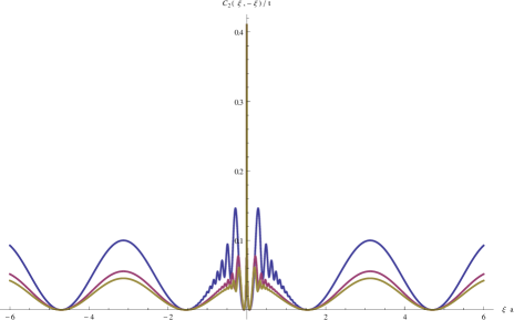
Figure 15: (Color online) Variation of $C_{2}$ for the attractive case with time. Note the growth of the central peak. At larger times, the correlations away from zero fall off. $ta^{2}=20,40,60$ for blue (top), magenta (middle) and yellow (bottom) respectively.

For more particles, we see interference fringes similar to the repulsive case. We note that the central peak increases and sharpens with time, indicating increasing contribution from bound states to the correlations (see Fig. 16 for an example).

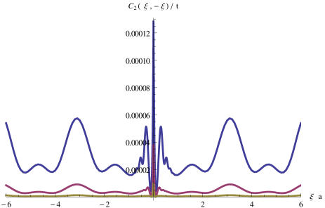
Figure 16: (Color online) $C_{2}(\xi,-\xi)$ for three particles in the attractive case plotted for three different times. At larger times, the correlations away from zero fall off. $ta^{2}=20,40,60$ for blue (top), magenta (middle) and yellow (bottom) respectively. (from Ref. Iyer and Andrei, 2012)

VI.3 Starting with a condensate - attractive and repulsive interactions

In this section, we study the evolution of the Bose gas after a quench from an initial state where all the bosons are in a single level of a harmonic trap. For $t<0$, the state is described by

$$\lvert\Psi_{\text{cond}}\rangle=\int_{x}\mathcal{S}_{x}\prod_{j}\frac{e^{-\frac{x_{j}^{2}}{\sigma^{2}}}}{(\pi\sigma^{2})^{\frac{1}{4}}}b^{\dagger}(x_{j})\lvert 0\rangle.$$ (VI.30)

Recall that in order to use the Yudson representation, the initial state needs to be ordered. We can rewrite the above state as

$$\lvert\Psi_{\text{cond}}\rangle=\int_{x}\theta(x_{1}>\cdots>x_{N})\\ \times\mathcal{S}_{x}\prod_{j}\frac{e^{-\frac{x_{j}^{2}}{\sigma^{2}}}}{(\pi\sigma^{2})^{\frac{1}{4}}}b^{\dagger}(x_{j})\lvert 0\rangle$$ (VI.31)

where $\mathcal{S}$ is a symmetrizer. The time evolution can be carried out via the Yudson representation, and again, we concentrate on the asymptotics. For the repulsive model, the stationary phase contribution is all that appears, and we get

$$\lvert\vec{x}\rangle=\int_{y}\prod_{i<j}S^{y}_{ij}\left(\frac{y_{i}-y_{j}-x_{i}+x_{j}}{2t}\right)\\ \prod_{j}\frac{1}{\sqrt{2\pi it}}e^{-i\frac{(y_{j}-x_{j})^{2}}{4t}+i\frac{(y_{j}-x_{j})^{2}}{2t}}b^{\dagger}(y_{j})\lvert 0\rangle.$$ (VI.32)

At large time $t$, we therefore have

$$\lvert\Psi_{\text{cond}}(t)\rangle=\int_{x,y}\theta(x_{1}>\cdots>x_{N})\phi_{2}(x)I(y,x,t)\\ \times\prod_{j}b^{\dagger}(y_{j})\lvert 0\rangle$$ (VI.33)

$\phi_{2}(x)$ is symmetric in $x$. $I(y,x,t)$ is symmetric in the $y$ but not in the $x$. Therefore we have to carry out the $x$ integration over the wedge $x_{1}>\cdots>x_{N}$. This is not straightforward to carry out. If $I(y,x,t)$ was also symmetric in $x$, then we can add the other wedges to rebuild the full space in $x$. However, due to the $S$-matrix factors, symmetrizing in $y$ does not automatically symmetrize in $x$. The exponential factors on the other hand are automatically symmetric in both variables if one of them is symmetrized because their functional dependence is of the form $f(y_{j}-x_{j})$. It is however possible to make the $S$-matrix factors approximately symmetric in $x$, and we will define what we mean by approximately shortly. What is important is to obtain a $y_{j}-x_{j}$ dependence. As of now, the $S$-matrix that appears in the above expression is

$$S^{y}_{ij}\left(\frac{y_{i}-y_{j}-x_{i}+x_{j}}{2t}\right)=\frac{\frac{y_{i}-y_{j}-x_{i}+x_{j}}{2t}-ic\operatorname{sgn}(y_{i}-y_{j})}{\frac{y_{i}-y_{j}-x_{i}+x_{j}}{2t}-ic}$$ (VI.34)

First, we can change $\operatorname{sgn}(y_{i}-y_{j})$ to $\operatorname{sgn}\left(\frac{y_{i}-y_{j}}{2t}\right)$ since $t>0$. Next, note that asymptotically in time, the stationary phase contribution comes from $\frac{y}{2t}\sim\mathcal{O}(1)$. However, since $x$ has finite extent, at large enough time, $\frac{x}{2t}\sim 0$. We are therefore justified in writing $\operatorname{sgn}\left(\frac{y_{i}-x_{i}}{2t}-\frac{y_{j}-x_{j}}{2t}\right)$. The only problem could arise when $y_{i}\sim y_{j}$. However, if this occurs, then the $S$-matrix is approximately $\operatorname{sgn}(y_{i}-y_{j})$ which is antisymmetric in $ij$. With this prefactor the particles are effectively fermions, and therefore at $y_{i}\sim y_{j}$, the wave-function has an approximate node. At large time therefore, we do not have to be concerned with the possibility of particles overlapping, and including the $x_{i}$ inside the $\operatorname{sgn}$ function is valid. With this change the $S$-matrix also becomes a function of $y_{j}-x_{j}$ and symmetrizing over $y$ one automatically symmetrizes over $x$.

In short, we have established that the wave function asymptotically in time can be made symmetric in $x$. This allows us to rebuild the full space. We get

$$\begin{split}\lvert\Psi_{\text{cond}}(t)\rangle&=\int_{x,y}\sum_{P}\theta(x_{P})\phi_{2}(x)I^{s}(y,x,t)\prod_{j}b^{\dagger}(y_{j})\lvert 0\rangle\\ &=\int_{x,y}\phi_{2}(x)I^{s}(y,x,t)\prod_{j}b^{\dagger}(y_{j})\lvert 0\rangle\end{split}$$ (VI.35)

where the $s$ superscript indicates that we have established that $I(y,x,t)$ is also symmetric in $x$. With this in mind, we can do away with the ordering when we’re integrating over the $x$ if we symmetrize the initial state wave function and the final wave function. Note that when we calculate the expectation value of a physical observable, the symmetry of the wavefunction is automatically enforced, and thus taken care of automatically.

Recall that when we calculated the noise correlations of the repulsive gas, in order to get an analytic expression for $N$ particles, we considered the leading order term, i.e., the HBT term. We did this by showing that higher order crossings produced terms higher order in $e^{-2ca}$ which we claimed was a small number. Now, however, $a=0$, and although the calculation is essentially the same with our approximate symmetrization, this simplification does not occur. The two and three particle results remain analytically calculable, but for higher numbers, we have to resort to numerical integration. Fig. 17 shows the noise correlation for two and three repulsive bosons starting from a condensate. For non-interacting particles, we expect a straight line $C_{2}=\frac{1}{2}$. When repulsive interactions are turned on, we see the characteristic fermionic dip develop. The plots for the attractive Bose gas are shown in Figs. 18 and 19. As expected from the non-interacting case the oscillations arising from the interference of particles separated spatially does not appear. The attractive however does show the oscillations near the central peak that are also visible in the case when we start from a lattice-like state. It is interesting to note that for three particles we do not see any additional structure develop in the attractive case.

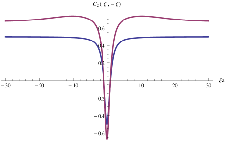
Figure 17: (Color online) $C_{2}(\xi,-\xi)$ for two (blue, bottom) and three (magenta, top)repulsive bosons starting from a condensate. Unlike the attractive case, there is no explicit time dependence asymptotically. $ca=3$ (from Ref. Iyer and Andrei, 2012)

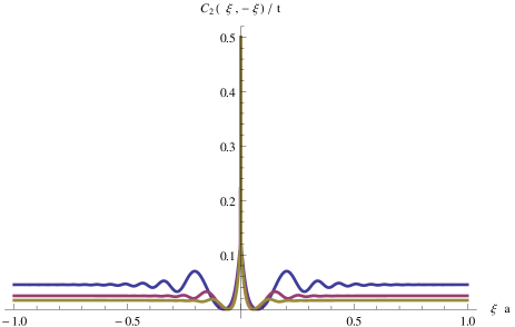
Figure 18: (Color online) Noise correlation for two attractive bosons starting from a condensate - as time increases from blue (top) to yellow (bottom), the central peak dominates.

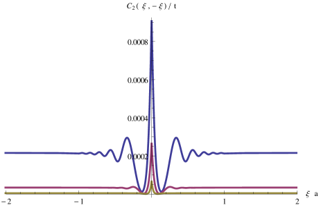
Figure 19: (Color online) $C_{2}(\xi,-\xi)$ for three attractive bosons starting from a condensate. Note that the side peak structure found in fig. 16 is missing due to the initial condition. We show the evolution at three times. As time increases, the oscillations near the central peak die out. Times from top to bottom $tc^{2}=20,40,60$. (from Ref. Iyer and Andrei, 2012)

VII Conclusions and the dynamic RG hypothesis

We have shown that the Yudson contour integral representation for arbitrary states can indeed be used to understand aspects of the quench dynamics of the Lieb-Liniger model, and obtain the asymptotic wave functions exactly. The representation overcomes some of the major difficulties involved in using the Bethe-Ansatz to study the dynamics of some integrable systems by automatically accounting for complicated states in the spectrum.

We see some interesting dynamical effects at long times. The infinite time limit of the repulsive model corresponds to particles evolving with a free fermionic Hamiltonian. It retains, however, memory of the initial state and therefore is not a thermal state. The correlation functions approach that of hard core bosons at long time indicating a dynamical increase in interaction strength. The attractive model also shows a dynamic strengthening of the interaction and the long time limit is dominated by a multiparticle bound state. This of course does not mean that it condenses. In fact the state diffuses over time, but remains strongly correlated.

We may interpret our results in terms of a “dynamic RG” in time. The asymptotic evolutions of the model both for $c>0$ and for $c<0$ are given by the Hamiltonians $H^{*}_{\pm}$ with $c\to\pm\infty$ respectively. Accepting the RG logic behind the conjecture one would expect that there would be basins of attraction around the Lieb-Liniger Hamiltonian with models whose long time evolution would bring them close to the ”dynamic fixed points” $H^{*}_{\pm}$. One such Hamiltonian would have short range potentials replacing the $\delta$-function interaction that renders the Lieb-Liniger model integrable. Perhaps, lattice models could be also found in this basin whose time asymptotics would be close, in the repulsive case, to that given by a free fermionic model on the lattice. Clearly, as discussed earlier, the Bose-Hubbard model is not such a model since it has a lattice symmetry that is not present in the Lieb-Liniger model. This could be however overcome by adding such terms as the next nearest hopping or interactions that break this symmetry, or as shown in Appendix A, with an appropriate choice of initial state.

We have to emphasize, however, that as these models are not integrable, we do not expect that they would actually flow to $H^{*}_{\pm}$. Instead, starting close enough in the “basin”, they would flow close to $H^{*}_{\pm}$ and spend much time in its neighborhood, eventually evolving into another, thermal state. We thus conjecture that away from integrability, a system would approach the corresponding non-thermal equilibrium, where the dynamics will slow down leading to a “prethermal” state Berges et al. (2004). Fig. 20 shows a schematic of this. Such prethermalization behavior has indeed been observed in lattice models Kollath et al. (2007). The system is expected to eventually find a thermal state. It is therefore of interest to characterize different ways of breaking integrability to see when a system is “too far” from integrability to see this effect and in what regimes a system can be considered as close to integrability. For a review and background on this subject, see Ref. Polkovnikov et al., 2011.

Further, the flow diagram in Fig. 20 might have another axis that represents initial states. Studying the Bose-Hubbard model shows an interesting initial state dependence. Whereas the sign of the interaction does not affect the quench dynamics, the asymptotic state depends strongly on the initial state, with a lattice-like state leading to fermionization, and a condensate-like state retaining bosonic correlations. The strong dependence on the initial state in the quench dynamics is evident from eq. (I.2) and is subject of much debate, in particular as relating to the Eigenstate Thermalization Hypothesis Rigol et al. (2008); Srednicki (1994); Deutsch (1991).

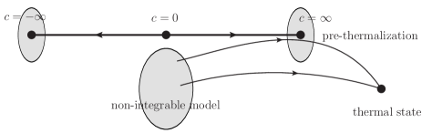
Figure 20: Schematic showing pre-thermalization of states in a non-integrable model

This work also opens up several new questions. It provides a prediction for experiments that can be carried out in the context of continuum cold atom systems (though the experiments we are aware of are carried out on the lattice and therefore described by the Bose-Hubbard model) Theoretically, while the representation is provable mathematically, further investigation is required to understand, physically, how it achieves the tedious sum over eigenstates, while automatically accounting for the details of the spectrum. This would allow us to extend the approach to other models with a more complicated $S$-matrix structure. It would also be useful to tie this approach to other means of calculating overlaps in the Algebraic Bethe Ansatz, i.e., the form-factor approach. The representation can essentially be thought of as a different way of writing the identity operator. From that standpoint, it could serve as a new way of evaluating correlation functions using the Bethe Ansatz. We are currently studying generalizations of this approach to other models that can be realized in optical lattices.

VIII Acknowledgments

We are grateful to G. Goldstein for very useful discussions. This work was supported by NSF grant DMR 1006684.

Appendix A Quenching the Bose-Hubbard model

We compare the results obtained in Section V with those from the lattice version of the Lieb-Liniger model - the Bose-Hubbard model,

$$H_{\text{BH}}=\sum_{i}\left[\left(tb^{{\dagger}}_{i}b_{i+1}+\text{h.c.}\right)+Un_{i}(n_{i}-1)\right]$$ (A.1)

It describe bosons $b$ hopping on a 1$d$ lattice with on-site interaction $U$ and is non-integrable since it allows multiparticle interactions on the same site. It has been extensively studied in many contexts and much is known about its equilibrium properties (see e.g., Ref. Kühner and Monien, 1998). For $0<U/t\ll 1$, the model is a superfluid, and for $U/t\gg 1$ it is a Mott insulator. For negative $U$, the model is attractive and the ground state is a Bose condensate. A non-equilibrium phase diagram of the Bose-Hubbard model is given in Ref. Kollath et al., 2007.

We study here the two boson quench dynamics and contrast it with the corresponding dynamics of the Lieb-Liniger model. Contrary to what one may expect, the introduction of the lattice modifies the dynamics in an essential way even at long times and distances. The calculations of density correlations as a function of time after a sudden quench have been carried out using the Algorithms and Libraries for Physics Simulations (ALPS) code http://alps.comp-phys.org ; Bauer et al. (2011); Albuquerque et al. (2007) and the Open source TEBD package http://physics.mines.edu/downloads/software/tebd/ after making the necessary modifications to accommodate the initial states we are interested in. Our results confirm some results obtained in Ref. Lahini et al., 2012.

In Fig. 21 we show the time evolution of the correlation matrix defined as $\langle n_{i}n_{j}\rangle$ after a sudden quench from an initial state $b^{{\dagger}}_{0}b^{{\dagger}}_{0}\lvert 0\rangle$, and in Fig. 22 the evolution from initial state $b^{{\dagger}}_{0}b^{{\dagger}}_{1}\lvert 0\rangle$. We quench into the interacting regime, where $|U|/t=10$. There are a couple of interesting features: (1) Unlike the situation in the Lieb-Liniger model where the bunching or anti-bunching effect is independent of the initial state, here, quenching a lattice-like state leads to anti-bunching Fig. 22, while quenching a condensate-like state leads to bunching Fig. 21. It is also interesting to compare the anti-bunching evolution of the bosons with the evolution of free fermions in Fig. 23.

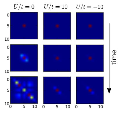
Figure 21: (Color online) Time evolution of the correlation matrix after a sudden quench from a state containing two bosons on the same site. The values increase from blue (0) to red. The correlations remain strong in the center indicating strong bunching.

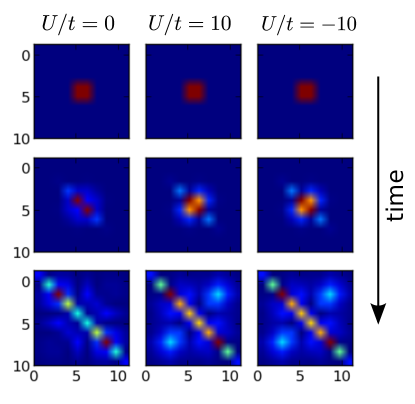
Figure 22: (Color online) Time evolution of the correlation matrix after a sudden quench from a state containing bosons on two neighboring sites. The values increase from blue (0) to red. The off diagonal correlations indicate anti-bunching, as can be seen from free fermion evolution in Fig. 23.

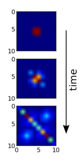
Figure 23: (Color online) Time evolution of free fermions on a lattice. Notice how off diagonal correlations develop. The values increase from blue (0) to red.

(2) The sign of the interaction plays no role in the evolution in the Bose-Hubbard model, as seen from either figures. This is unlike the situation in the continuum model where for repulsive interactions anti-bunching (fermionization) occurs independently of the initial state, while bunching will take place for attractive interactions.

This non-dependence on the sign of the interaction is due to a particle-hole symmetry that is present on the lattice, but not in the continuum. The 1$d$ lattice, being bipartite, allows the the transformation $b_{j}\to e^{i\pi j}b_{j}$, with$j$ the site index, under which the hopping terms pick up a minus sign, while the on-site interaction terms are unaffected, thus $U/t\to-U/t$. In terms of $\mathcal{U}$ the corresponding unitary operator we have,

$$\mathcal{U}H_{\text{BH}}(t,-U)\mathcal{U}^{{\dagger}}=-H_{\text{BH}}\,(t,U).$$ (A.2)

Denoting eigenstates and eigenvalues of $H_{\text{BH}}(t,U)\equiv H_{\text{BH}}$ by $\lvert m\rangle$ and $\epsilon_{m}$ and the corresponding eigenstates and eigenvalues of $H_{\text{BH}}(t,-U)\equiv\tilde{H}_{\text{BH}}$ by $\lvert\tilde{m}\rangle$ and $\tilde{\epsilon}_{m}$ we can relate the states by: $\lvert\tilde{m}\rangle=\mathcal{U}\lvert m\rangle$, and the eigenvalues by: $\tilde{\epsilon}_{m}=-\epsilon_{m}$. The time evolution of an operator $\mathcal{O}$ under the action of $H_{\text{BH}}(t,U)$ from an initial state $\lvert\Psi_{0}\rangle$

$$\langle\mathcal{O}(t)\rangle_{H}=\sum_{m,m^{\prime}}\langle\Psi_{0}|m^{\prime}\rangle\langle m|\Psi_{0}\rangle\langle m^{\prime}\rvert\mathcal{O}\lvert m\rangle e^{-i(\epsilon_{m}-\epsilon_{m^{\prime}})t}$$ (A.3)

Under $\tilde{H}_{\text{BH}}$,

$$\begin{split}&\langle\mathcal{O}(t)\rangle_{\tilde{H}}=\sum_{\tilde{m},\tilde{m}^{\prime}}\langle\Psi_{0}|\tilde{m}^{\prime}\rangle\langle\tilde{m}|\Psi_{0}\rangle\langle\tilde{m}^{\prime}\rvert\mathcal{O}\lvert\tilde{m}\rangle e^{-i(\tilde{\epsilon}_{m}-\tilde{\epsilon_{m^{\prime}}})t}\\ &=\sum_{m,m^{\prime}}\langle\Psi_{0}\rvert\mathcal{U}\lvert m^{\prime}\rangle\langle m\rvert\mathcal{U}^{{\dagger}}\lvert\Psi_{0}\rangle\langle m^{\prime}\rvert\mathcal{U}^{{\dagger}}\mathcal{O}\mathcal{U}\lvert m\rangle e^{i(\epsilon_{m}-\epsilon_{m^{\prime}})t}\end{split}$$ (A.4)

Both initial state we considered, $\lvert\Psi_{\text{latt}}\rangle=b_{0}^{{\dagger}}b_{1}^{{\dagger}}\lvert 0\rangle$ and $\lvert\Psi_{\text{cond}}\rangle=(b^{{\dagger}}_{0})^{2}\lvert 0\rangle$ are simply transformed, $\mathcal{U}\lvert\Psi_{0}\rangle=\pm\lvert\Psi_{0}\rangle$ and as they occur twice in the overlaps the transformation leaves no effect. Similarly the operators we have considered (density-density correlations) are bilinear in the site operators and are therefore not affected, $\mathcal{U}^{{\dagger}}\mathcal{O}\mathcal{U}=\mathcal{O}$. This gives

$$\langle\mathcal{O}(t)\rangle_{\tilde{H}}=\sum_{m,m^{\prime}}\langle\Psi_{0}\lvert m^{\prime}\rangle\langle m\lvert\Psi_{0}\rangle\langle m^{\prime}\rvert\mathcal{O}\lvert m\rangle e^{i(\epsilon_{m}-\epsilon_{m^{\prime}})t}$$ (A.5)

Next, we note that the Bose-Hubbard Hamiltonian is invariant under time reversal, i.e., $[H_{\text{BH}},\mathcal{T}]=0$ where $\mathcal{T}$ is the anti-unitary time reversal operator:

$$\mathcal{T}t\mathcal{T}^{-1}=-t,\qquad\mathcal{T}i\mathcal{T}^{-1}=-i.$$ (A.6)

Applying the time reversal operator to the expectation value above, we get

$$\begin{split}&\langle\mathcal{O}(t)\rangle_{\tilde{H}}=\mathcal{T}\langle\mathcal{O}(t)\rangle_{\tilde{H}}\mathcal{T}^{-1}\\ &=\sum_{m,m^{\prime}}\langle\Psi_{0}\lvert m^{\prime}\rangle^{*}\langle m\lvert\Psi_{0}\rangle^{*}\langle m^{\prime}\rvert\mathcal{O}\lvert m\rangle^{*}e^{i(\epsilon_{m}-\epsilon_{m^{\prime}})t}\\ &=\sum_{m,m^{\prime}}\langle\Psi_{0}\lvert m\rangle\langle m^{\prime}\lvert\Psi_{0}\rangle\langle m\rvert\mathcal{O}\lvert m^{\prime}\rangle e^{i(\epsilon_{m}-\epsilon_{m^{\prime}})t}\\ &=\sum_{m,m^{\prime}}\langle\Psi_{0}\lvert m^{\prime}\rangle\langle m\lvert\Psi_{0}\rangle\langle m^{\prime}\rvert\mathcal{O}\lvert m\rangle e^{-i(\epsilon_{m}-\epsilon_{m^{\prime}})t}\\ &=\langle\mathcal{O}(t)\rangle_{H}\end{split}$$ (A.7)

thus indeed, the time evolution looks the same for both signs of the interaction. Note that with initial states or operators that are not invariant (up to a sign) under the transformation $\mathcal{U}$, we should see a difference in the time evolution of the attractive and repulsive models.

A similar symmetry exists in the XXZ model or the Hubbard model in 1$d$ (or higher dimensional bipartite lattices). For the magnet, the

sign of the anisotropy $\Delta$ leads to either ferromagnetic or antiferromagnetic ground states for negative or positive anisotropy. However, it does not influence the quench dynamics Barmettler et al. (2010), as can be seen from arguments like the above. Similarly in the Hubbard model, the quench dynamics is unaffected by the change of sign of $U$ Schneider et al. (2012).

References

- De Groot and Mazur (2012) S. R. De Groot and P. Mazur, Non-equilibrium Thermodynamics (Dover Publications, 2012).
- Bloch et al. (2008) I. Bloch, J. Dalibard, and W. Zwerger, Rev. Mod. Phys. 80, 885 (2008).
- Note (1) In the broader sense transport may be viewed as the long time limit of quench. For example, a steady state current would result if we quench a quantum dot attaching it to two leads held at different chemical potentials Doyon and Andrei (2006).
- Rigol (2009) M. Rigol, Phys. Rev. Lett. 103, 100403 (2009).
- Rigol et al. (2008) M. Rigol, V. Dunjko, and M. Olshanii, Nature 451, 854 (2008).
- Calabrese and Caux (2007) P. Calabrese and J.-S. Caux, Journal of Statistical Mechanics: Theory and Experiment 2007, P08032 (2007).
- Mossel and Caux (2012) J. Mossel and J.-S. Caux, arXiv:1201.1885 cond-mat.stat-mech (2012).
- White and Feiguin (2004) S. R. White and A. E. Feiguin, Phys. Rev. Lett. 93, 076401 (2004).
- Daley et al. (2004) A. J. Daley, C. Kollath, U. Schollwöck, and G. Vidal, Journal of Statistical Mechanics: Theory and Experiment 2004, P04005 (2004).
- Kinoshita et al. (2006) T. Kinoshita, T. Wenger, and D. S. Weiss, Nature 440, 900 (2006).
- Bethe (1931) H. Bethe, Zeitschrift für Physik A Hadrons and Nuclei 71, 205 (1931), 10.1007/BF01341708.
- Takahashi (1999) M. Takahashi, Thermodynamics of One Dimensional Solvable Models (Cambridge University Press, 1999).
- Andrei et al. (1983) N. Andrei, K. Furuya, and J. H. Lowenstein, Rev. Mod. Phys. 55, 331 (1983).
- Tsvelick and Wiegmann (1983) A. Tsvelick and P. Wiegmann, Advances in Physics 32, 453 (1983).
- Andrei (1995) N. Andrei, in Low-Dimensional Quantum Field Theories for Condensed Matter Physicists: Lecture Notes of ICTP Summer Course Trieste, Italy September 1992, Series on Modern Condensed Matter Physics, Vol. 6, edited by S. Lundqvist, G. Morandi, L. Yü, and I. C. for Theoretical Physics (World Scientific, 1995).
- Yudson (1985) V. I. Yudson, Soviet Physics JETP 61, 1043 (1985).
- Yudson (1988) V. I. Yudson, Physics Letters A 129, 17 (1988).
- Lieb and Liniger (1963) E. H. Lieb and W. Liniger, Phys. Rev. 130, 1605 (1963).
- Iyer and Andrei (2012) D. Iyer and N. Andrei, Phys. Rev. Lett. 109, 115304 (2012).
- Lahini et al. (2012) Y. Lahini, M. Verbin, S. D. Huber, Y. Bromberg, R. Pugatch, and Y. Silberberg, Phys. Rev. A 86, 011603 (2012).
- Barmettler et al. (2010) P. Barmettler, M. Punk, V. Gritsev, E. Demler, and E. Altman, New Journal of Physics 12, 055017 (2010).
- Giamarchi (2004) T. Giamarchi, Quantum Physics in One Dimension, edited by J. Birman, S. F. Edwards, R. Friend, M. Rees, D. Sherrington, and G. Veneziano, The International Series of Monographs on Physics (Oxford University Press, 2004).
- Note (2) One can refine the estimate for the interaction time setting , with . Also if we start from a lattice-like state, will include a short time scale before which the system only expands as a non-interacting gas, until neighboring wave-functions overlap sufficiently.
- Rigol et al. (2007) M. Rigol, V. Dunjko, V. Yurovsky, and M. Olshanii, Phys. Rev. Lett. 98, 050405 (2007).
- Calabrese and Cardy (2007) P. Calabrese and J. Cardy, Journal of Statistical Mechanics: Theory and Experiment 2007, P10004 (2007).
- Caux and Essler (2013) J.-S. Caux and F. H. L. Essler, (2013), arXiv:1301.3806 .
- Caux and Konik (2012) J.-S. Caux and R. M. Konik, Phys. Rev. Lett. 109, 175301 (2012).
- Lieb and Wu (1968) E. H. Lieb and F. Y. Wu, Phys. Rev. Lett. 20, 1445 (1968).
- Note (3) This set of conditions is known as the Yang-Baxter equation.
- Sklyanin et al. (1979) E. K. Sklyanin, L. A. Takhtadzhyan, and L. D. Faddeev, Theoretical and Mathematical Physics 40, 688 (1979), 10.1007/BF01018718.
- Korepin et al. (1997) V. E. Korepin, N. M. Bogoliubov, and A. G. Izergin, Quantum Inverse Scattering Method and Correlation Functions (Cambridge Monographs on Mathematical Physics) (Cambridge University Press, 1997).
- Thacker (1981) H. B. Thacker, Rev. Mod. Phys. 53, 253 (1981).
- Gritsev et al. (2010) V. Gritsev, T. Rostunov, and E. Demler, Journal of Statistical Mechanics: Theory and Experiment 2010, P05012 (2010).
- Cazalilla et al. (2011) M. A. Cazalilla, R. Citro, T. Giamarchi, E. Orignac, and M. Rigol, Rev. Mod. Phys. 83, 1405 (2011).
- Görlitz et al. (2001) A. Görlitz, J. M. Vogels, A. E. Leanhardt, C. Raman, T. L. Gustavson, J. R. Abo-Shaeer, A. P. Chikkatur, S. Gupta, S. Inouye, T. Rosenband, and W. Ketterle, Phys. Rev. Lett. 87, 130402 (2001).
- Moritz et al. (2003) H. Moritz, T. Stöferle, M. Köhl, and T. Esslinger, Phys. Rev. Lett. 91, 250402 (2003).
- Girardeau (1960) M. Girardeau, J. Math. Phys. 1, 516 (1960).
- Dicke (1954) R. H. Dicke, Phys. Rev. 93, 99 (1954).
- Tracy and Widom (2008) C. A. Tracy and H. Widom, Journal of Physics A: Mathematical and Theoretical 41, 485204 (2008).
- Lamacraft (2011) A. Lamacraft, Phys. Rev. A 84, 043632 (2011).
- Prolhac and Spohn (2011) S. Prolhac and H. Spohn, Journal of Mathematical Physics 52, 122106 (2011).
- Yang (1968) C. N. Yang, Phys. Rev. 168, 1920 (1968).
- Hanbury-Brown and Twiss (1956) R. Hanbury-Brown and R. Q. Twiss, Nature 177, 27 (1956).
- Jukić et al. (2008) D. Jukić, R. Pezer, T. Gasenzer, and H. Buljan, Phys. Rev. A 78, 053602 (2008).
- Berges et al. (2004) J. Berges, S. Borsányi, and C. Wetterich, Phys. Rev. Lett. 93, 142002 (2004).
- Kollath et al. (2007) C. Kollath, A. M. Läuchli, and E. Altman, Phys. Rev. Lett. 98, 180601 (2007).
- Polkovnikov et al. (2011) A. Polkovnikov, K. Sengupta, A. Silva, and M. Vengalattore, Rev. Mod. Phys. 83, 863 (2011).
- Srednicki (1994) M. Srednicki, Phys. Rev. E 50, 888 (1994).
- Deutsch (1991) J. M. Deutsch, Phys. Rev. A 43, 2046 (1991).
- Kühner and Monien (1998) T. D. Kühner and H. Monien, Phys. Rev. B 58, R14741 (1998).
- (51) http://alps.comp-phys.org, .
- Bauer et al. (2011) B. Bauer, L. D. Carr, H. G. Evertz, A. Feiguin, J. Freire, S. Fuchs, L. Gamper, J. Gukelberger, E. Gull, S. Guertler, A. Hehn, R. Igarashi, S. V. Isakov, D. Koop, P. N. Ma, P. Mates, H. Matsuo, O. Parcollet, G. Pawłowski, J. D. Picon, L. Pollet, E. Santos, V. W. Scarola, U. Schollwöck, C. Silva, B. Surer, S. Todo, S. Trebst, M. Troyer, M. L. Wall, P. Werner, and S. Wessel, Journal of Statistical Mechanics: Theory and Experiment 2011, P05001 (2011).
- Albuquerque et al. (2007) A. Albuquerque, F. Alet, P. Corboz, P. Dayal, A. Feiguin, S. Fuchs, L. Gamper, E. Gull, S. Gürtler, A. Honecker, R. Igarashi, M. Körner, A. Kozhevnikov, A. Läuchli, S. Manmana, M. Matsumoto, I. McCulloch, F. Michel, R. Noack, G. P. owski, L. Pollet, T. Pruschke, U. Schollwöck, S. Todo, S. Trebst, M. Troyer, P. Werner, and S. Wessel, Journal of Magnetism and Magnetic Materials 310, 1187 (2007), proceedings of the 17th International Conference on Magnetism.
- (54) http://physics.mines.edu/downloads/software/tebd/, .
- Schneider et al. (2012) U. Schneider, L. Hackermüller, J. P. Ronzheimer, S. Will, S. Braun, T. Best, I. Bloch, E. Demler, S. Mandt, D. Rasch, and A. Rosch, Nature Physics 8, 213 (2012), arXiv:1005.3545 [cond-mat.quant-gas] .
- Doyon and Andrei (2006) B. Doyon and N. Andrei, Phys. Rev. B 73, 245326 (2006).