Distributing Entanglement with Separable States

Abstract

We experimentally demonstrate a protocol for entanglement distribution by a separable quantum system. In our experiment, two spatially separated modes of an electromagnetic field get entangled by local operations, classical communication, and transmission of a correlated but separable mode between them. This highlights the utility of quantum correlations beyond entanglement for the establishment of a fundamental quantum information resource and verifies that its distribution by a dual classical and separable quantum communication is possible.

Like a silver thread, quantum entanglement Schrodinger_35 runs through the foundations and breakthrough applications of quantum information theory. It cannot arise from local operations and classical communication (LOCC) and therefore represents a more intimate relationship among physical systems than we may encounter in the classical world. The “nonlocal” character of entanglement manifests itself through a number of counterintuitive phenomena encompassing the Einstein-Podolsky-Rosen paradox Einstein_35 ; Reid_89 , steering Wiseman_07 , Bell nonlocality Bell_64 , or negativity of entropy Cerf_97 ; MHorodecki_05 . Furthermore, it extends our abilities to process information. Here, entanglement is used as a resource which needs to be shared between remote parties. However, entanglement is not the only manifestation of quantum correlations. Notably, separable quantum states can also be used as a shared resource for quantum communication. The experiment presented in this Letter highlights the quantumness of correlations in separable mixed states and the role of classical information in quantum communication by demonstrating entanglement distribution using merely a separable ancilla mode.

The role of entanglement in quantum information is nowadays vividly demonstrated in a number of experiments. A pair of entangled quantum systems shared by two observers enables us to teleport Bennett_93 quantum states between them with a fidelity beyond the boundary set by classical physics. Concatenated teleportations Zukowski_93 can further span entanglement over large distances Briegel_98 which can be subsequently used for secure communication Ekert_91 . An a priori shared entanglement also allows us to double the rate at which information can be sent through a quantum channel Bennett_92 or one can fuse bipartite entanglement into larger entangled cluster states that are “hardware” for quantum computing Raussendorf_01 .

The common feature of all entangling methods used so far is that entanglement is either produced by some global operation on the systems that are to be entangled or it results from a direct transmission of entanglement (possibly mediated by a third system) between the systems. Even entanglement swapping Zukowski_93 ; Pan_98 , capable of establishing entanglement between the systems that do not have a common past, is not an exception to the rule because also here entanglement is directly transmitted between the participants.

However, quantum mechanics admits conceptually different means of establishing entanglement which are free of transmission of entanglement. Remarkably, the creation of entanglement between two observers can be disassembled into local operations and the communication of a separable quantum system between them Cubitt_03 . The impossibility of entanglement creation by LOCC is not violated because communication of a quantum system is involved. The corresponding protocol exists only in a mixed-state scenario and obviously utilizes fewer quantum resources in comparison with the previous cases because communication of only a discordant Streltsov_12 ; Chuan_12 ; Kay_12 separable quantum system is required.

In this Letter, we experimentally demonstrate the entanglement distribution by a separable ancilla Cubitt_03 with Gaussian states of light modes Mista_09 . The protocol aims at entangling mode $A$ which is in possession of a sender Alice, with mode $B$ held by a distant receiver Bob by local operations and transmission of a separable mediating mode $C$ from Alice to Bob. This requires the parties to prepare their initial modes $A$, $B$, and $C$ in a specific correlated but fully separable Gaussian state. Once the resource state $\hat{\rho}_{ABC}$ is established, no further classical communication is needed to accomplish the protocol. To emphasize this, we attribute the state preparation process to a separate party, David. Note that this resource state preparation is performed by LOCC only. No global quantum operation with respect to David’s separated boxes is executed at the initial stage, and no entanglement is present.

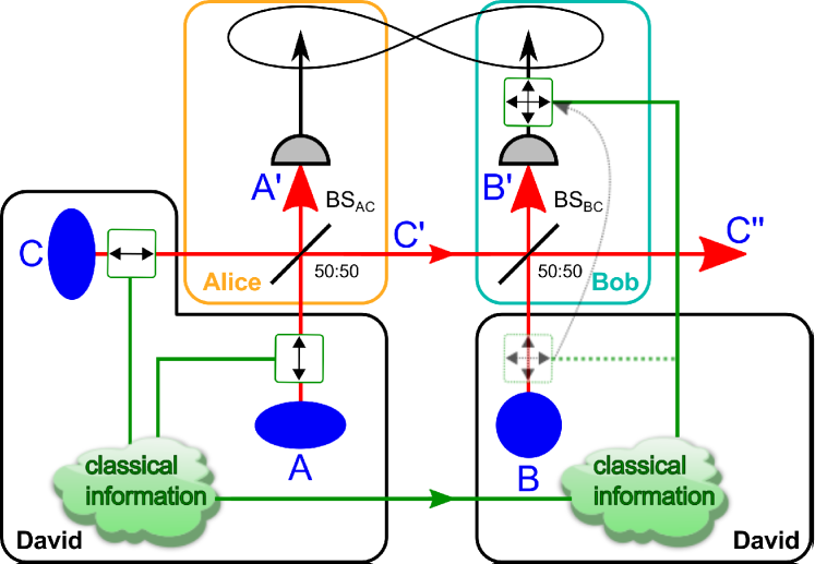
Figure 1: Sketch of the Gaussian entanglement distribution protocol. David prepares a momentum squeezed vacuum mode $A$, a position squeezed vacuum mode $C$, and a vacuum mode $B$. He then applies random displacements (green boxes) of the $\hat{x}$ quadrature (horizontal arrow) and the $\hat{p}$ quadrature (vertical arrow) as in Eq. (Protocol.), which are correlated via a classical communication channel (green line). David passes modes $A$ and $C$ to Alice and mode $B$ to Bob. Alice superimposes modes $A$ and $C$ on a balanced beam splitter BS_AC and communicates the separable output mode $C^{\prime}$ to Bob (red line connecting Alice and Bob). Bob superimposes the received mode $C^{\prime}$ with his mode $B$ on another balanced beam splitter BS_BC, which establishes entanglement between the output modes $A^{\prime}$ and $B^{\prime}$ (black lemniscata). Note the position of the displacement on mode $B$. In the original protocol, the displacement is performed before BS_BC, which is depicted by the corresponding box with a dashed green line. Equivalently, this displacement on mode $B$ can be performed after BS_BC (dashed arrow indicates the respective relocation of displacement) on mode $B^{\prime}$, and even a posteriori after the measurement of mode $B^{\prime}$.

Protocol.

The protocol Mista_09 depicted in Fig. 1 consists of three steps. Initially, a distributor David prepares modes $A$ and $C$ in momentum squeezed and position squeezed vacuum states, respectively, with quadratures $\hat{x}_{A,C}=e^{\pm r}\hat{x}_{A,C}^{(0)}$ and $\hat{p}_{A,C}=e^{\mp r}\hat{p}_{A,C}^{(0)}$, whereas mode $B$ is in a vacuum state with quadratures $\hat{x}_{B}=\hat{x}_{B}^{(0)}$ and $\hat{p}_{B}=\hat{p}_{B}^{(0)}$. Here, $r$ is the squeezing parameter and the superscript $(0)$ denotes the vacuum quadratures. David then exposes all the modes to suitably tailored local correlated displacements Mista_12 :

$$\hat{p}_{A} \rightarrow \hat{p}_{A}-p,\quad\hat{x}_{C}\rightarrow\hat{x}_{C}+x,$$

$$\hat{x}_{B} \rightarrow \hat{x}_{B}+\sqrt{2}x,\quad\hat{p}_{B}\rightarrow\hat{p}_{B}+\sqrt{2}p.$$ (1)

The uncorrelated classical displacements $x$ and $p$ obey a zero mean Gaussian distribution with the same variance $(e^{2r}-1)/2$. The state has been prepared by LOCC across $A|B|C$ splitting and hence is fully separable.

In the second step, David passes modes $A$ and $C$ of the resource state to Alice and mode $B$ to Bob. Alice superimposes modes $A$ and $C$ on a balanced beam splitter BS_AC, whose output modes are denoted by $A^{\prime}$ and $C^{\prime}$. The beam splitter BS_AC cannot create entanglement with mode $B$. Hence the state is separable with respect to $B|A^{\prime}C^{\prime}$ splitting. Moreover, the state also fulfils the positive partial transpose (PPT) criterion Peres96 ; Horodecki96 with respect to mode $C^{\prime}$ and hence is also separable across $C^{\prime}|A^{\prime}B$ splitting Werner_01 , as required (see Appendix).

In the final step, Alice sends mode $C^{\prime}$ to Bob who superimposes it with his mode $B$ on another balanced beam splitter BS_BC. The presence of the entanglement between modes $A^{\prime}$ and $B^{\prime}$ is confirmed by the sufficient condition for entanglement Giovannetti_03 ; Dong_07

$$\Delta_{\rm norm}^{2}(g\hat{x}_{A^{\prime}}+\hat{x}_{B^{\prime}})\Delta_{\rm norm}^{2}(g\hat{p}_{A^{\prime}}-\hat{p}_{B^{\prime}})<1,$$ (2)

where $g$ is a variable gain factor. Minimizing the left-hand side of Ineq. (2) with respect to $g$, we get fulfilment of the criterion for any $r>0$, which confirms successful entanglement distribution.

Experiment.

The experimental realization is divided into three steps: state preparation, measurement, and data processing. The corresponding setup is depicted in Fig. 2. From now on, we will work with polarization variables described by Stokes observables (see, e.g., Refs. Korolkova_02 ; Heersink_05 ) instead of quadratures. We choose the state of polarization such that mean values of $\hat{S}_{1}$ and $\hat{S}_{2}$ equal zero while $\langle\hat{S}_{3}\rangle\gg 0$. This configuration allows us to identify the “dark” $\hat{S}_{1}$-$\hat{S}_{2}$ plane with the quadrature phase space. $\hat{S}_{\theta},\hat{S}_{\theta+\pi/2}$ in this plane correspond to $\hat{S}_{1},\hat{S}_{2}$ renormalized with respect to $\hat{S}_{3}\approx S_{3}$ and can be associated with the effective quadratures $\hat{x},\hat{p}$. We use the modified version of the protocol indicated in Fig. 1 by the dashed arrow showing the alternative position of displacement in mode $B$: The random displacement applied by David can be performed after the beam splitter interaction of $B$ and $C^{\prime}$, even a posteriori after the measurement of mode $B^{\prime}$. This is technically more convenient and emphasizes that the classical information is sufficient for the entanglement recovery after the interaction of mode $A$ with mode $C$ and mode $B$ with mode $C^{\prime}$.

David prepares two identically polarization squeezed modes Heersink_05 ; Leuchs99 ; Silberhorn01 ; Dong_07 and adds noise in the form of random displacements to the squeezed observables. The technical details on the generation of these modes can be found in the Appendix. The modulation patterns applied to modes $A$ and $C$ to implement the random displacements are realized using electro-optical modulators (EOMs) and are chosen such that the two-mode state $\hat{\rho}_{A^{\prime}C^{\prime}}$ is separable. By applying a sinusoidal voltage $V_{\text{mod}}$, the birefringence of the EOMs changes at a frequency of 18.2 MHz. In this way, the state is modulated along the direction of its squeezed observable.

Two such identically prepared modes $A$ and $C$ are interfered on a balanced beam splitter (BS_AC) with a fixed relative phase of $\pi/2$ by controlling the optical path length of one mode with a piezoelectric transducer and a locking loop. This results in equal intensities of both output modes. In the final step, Bob mixes the ancilla mode $C^{\prime}$ with a vacuum mode $B$ on another balanced beam splitter and performs a measurement on the transmitted mode $B^{\prime}$.

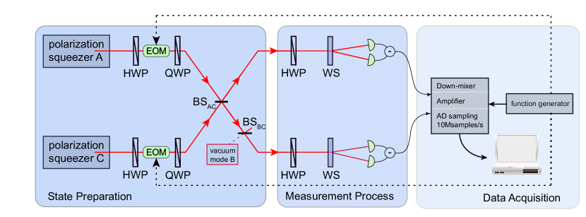
Figure 2: Sketch of the experimental setup. Used abbreviations: HWP, half-wave plate; QWP, quarter-wave plate; EOM, electro-optical modulator; BS, beam splitter; WS, Wollaston prism; and AD, analog-to-digital. State preparation: The polarization of two polarization squeezed states ($A$ and $C$) is modulated using EOMs and sinusoidal voltages from a function generator (dotted lines). The HWPs before the EOMs are used to adjust the direction of modulation to the squeezed Stokes variable, whereas the QWPs compensate for the stationary birefringence of the EOMs. Such prepared modes interfere with a relative phase of $\pi/2$ on a balanced beam splitter BS_AC. In the last step of the protocol, the mode $C^{\prime}$ interferes with the vacuum mode $B$ on a second balanced beam splitter BS_BC. Measurement process: A rotatable HWP, followed by a WS and a pair of detectors, from which the difference signal is taken, allows us to measure all possible Stokes observables in the $\hat{S}_{1}$-$\hat{S}_{2}$ plane. To determine the two-mode covariance matrix $\gamma_{A^{\prime}B^{\prime}}$, all necessary combinations of Stokes observables are measured. Removing the second beam splitter of the state preparation allows us to measure the covariance matrix of the two-mode state $\hat{\rho}_{A^{\prime}C^{\prime}}$. Data acquisition To achieve displacements of the modes in the $\hat{S}_{1}$-$\hat{S}_{2}$ plane we electronically mix the Stokes signals with a phase matched electrical local oscillator and sample them by an analog-to-digital converter.

The states involved are Gaussian quantum states and, hence, are completely characterized by their first moments and the covariance matrix $\gamma$ comprising all second moments (see Appendix). To study the correlations between modes $A^{\prime}$ and $C^{\prime}$ after BS_AC, multiple pairs of Stokes observables ($\hat{S}_{A^{\prime},\theta},\hat{S}_{C^{\prime},\theta}$) are measured. The covariance matrix $\gamma_{A^{\prime}C^{\prime}}$ is obtained by measuring five pairs of observables: $(\hat{S}_{A^{\prime},0^{\circ}},\hat{S}_{C^{\prime},0^{\circ}})$, $(\hat{S}_{A^{\prime},90^{\circ}},\hat{S}_{C^{\prime},0^{\circ}})$, $(\hat{S}_{A^{\prime},0^{\circ}},\hat{S}_{C^{\prime},90^{\circ}})$, $(\hat{S}_{A^{\prime},90^{\circ}},\hat{S}_{C^{\prime},90^{\circ}})$, and $(\hat{S}_{A^{\prime},45^{\circ}},\hat{S}_{C^{\prime},45^{\circ}})$, which determine all of its 10 independent elements. Here, $\theta$ is the angle in the $\hat{S}_{1}$-$\hat{S}_{2}$ plane between $\hat{S}_{0^{\circ}}$ and $\hat{S}_{\theta}$.

For the measurements of the different Stokes observables, we use two Stokes measurement setups, each comprising a rotatable half-wave plate, a Wollaston prism, and two balanced detectors. The difference signal of one pair of detectors gives one Stokes observable $\hat{S}_{\theta}$ in the $\hat{S}_{1}$-$\hat{S}_{2}$ plane, depending on the orientation of the half-wave plate. The signals are electrically down-mixed using an electric local oscillator at 18.2 MHz, which is in phase with the modulation used in the state preparation step. With this detection scheme, the modulation translates to a displacement of the states in the $\hat{S}_{1}$-$\hat{S}_{2}$ plane. The difference signal is low pass filtered (1.9 MHz), amplified, and then digitized using an analog-to-digital converter card (GaGe Compuscope 1610) at a sampling rate of $10^{6}$ samples/s. After the measurement process, we digitally low pass filter the data by an average filter with a window of 10 samples.

Because of the ergodicity of the problem, we are able to create a Gaussian mixed state computationally from the data acquired as described above. By applying $80$ different modulation depths $V_{\text{mod}}$ to each of the EOMs we acquire a set of $6400$ different modes. From this set of modes, we take various amounts of samples, weighted by a two-dimensional Gaussian distribution.

The covariance matrix $\gamma_{A^{\prime}C^{\prime}}$ for the two-mode state after BS_AC has been measured to be

$$\gamma_{A^{\prime}C^{\prime}}=\begin{pmatrix}20.90&1.102&-7.796&-1.679\\ 1.102&25.30&1.000&14.63\\ -7.796&1.000&20.68&0.8010\\ -1.679&14.63&0.8010&24.65\end{pmatrix}.$$ (3)

The estimation of the statistical errors of this covariance matrix $\gamma_{A^{\prime}C^{\prime}}$ can be found in the Appendix. A necessary and sufficient condition for the separability of a Gaussian state $\hat{\rho}_{XY}$ of two modes $X$ and $Y$ with the covariance matrix $\gamma_{XY}$ is given by the PPT criterion

$$\gamma_{XY}^{(T_{Y})}+i\Omega_{2} \geq 0,\quad\Omega_{2} =\bigoplus_{i=1}^{2}\left(\begin{array}[]{cc}0&1\\ -1&0\\ \end{array}\right)$$ (6)

where $\gamma_{XY}^{(T_{Y})}$ is the matrix corresponding to the partial transpose of the state $\hat{\rho}_{XY}$ with respect to the mode $Y$ (see Appendix). Effects that could possibly lead to some non-Gaussianity of the utilized states are also discussed in detail in the Appendix. The state described by $\gamma_{A^{\prime}C^{\prime}}$ fulfils the condition (6) as the eigenvalues (39.84, 28.47, 13.85, and 9.371) of $(\gamma_{A^{\prime}C^{\prime}}^{(T_{C^{\prime}})}+i\Omega_{2})$ are positive; hence, mode $C^{\prime}$ remains separable after BS_AC.

The measured two-mode covariance matrix of the output state $\gamma_{A^{\prime}B^{\prime}}$ is given by

$$\gamma_{A^{\prime}B^{\prime}}=\begin{pmatrix}19.95&1.025&-4.758&-1.063\\ 1.025&22.92&0.9699&9.153\\ -4.758&0.9699&9.925&0.2881\\ -1.063&9.153&0.2881&11.65\end{pmatrix}.$$ (7)

The statistical error of this measured covariance matrix is given in the Appendix. The separability is proven by the PPT criterion (eigenvalues 28.24, 21.79, 8.646, and 5.756).

The postprocessing for the recovery of the entanglement is performed on the measured raw data of mode $B^{\prime}$. Therefore, the displacement of the individual modes caused by the two modulators is calibrated. By means of this calibration, suitable displacements are applied digitally. The classical noise inherent in mode $B^{\prime}$ is completely removed. A part of the classical noise associated with $\hat{S}_{A^{\prime},0^{\circ}}$ is subtracted from $\hat{S}_{B^{\prime},0^{\circ}}$, while the same fraction of the noise in $\hat{S}_{A^{\prime},90^{\circ}}$ is added to $\hat{S}_{B^{\prime},90^{\circ}}$. In this way, the noise partially cancels out in the calculation of the separability criterion (2) and allows us to reveal the entanglement. We chose the fraction as in Eq. (Protocol.), which is compatible with the separability of the transmitted mode $C^{\prime}$ from the subsystem $(A^{\prime}B)$ in the scenario with modulation on mode $B$ before the beam splitter BS_BC.

Only as Bob receives the classical information about the modulation on the initial modes $A$ and $C$ from David is he able to recover the entanglement between $A^{\prime}$ and $B^{\prime}$. Bob verifies that the product entanglement criterion (2) is fulfilled, as illustrated in Fig. 3. That proves the emergence of entanglement. The used gain factor $g$ considers the slightly different detector response and the intentional loss of 50 % at Bob’s beam splitter. The clearest confirmation of entanglement $0.6922\pm 0.0002<1$ is shown for $g_{\text{opt}}=0.4235\pm 0.0005$ (Fig. 3). This is the only step of the protocol, where entanglement emerges, thus demonstrating the remarkable possibility to entangle remote parties Alice and Bob solely by sending a separable auxiliary mode $C^{\prime}$.

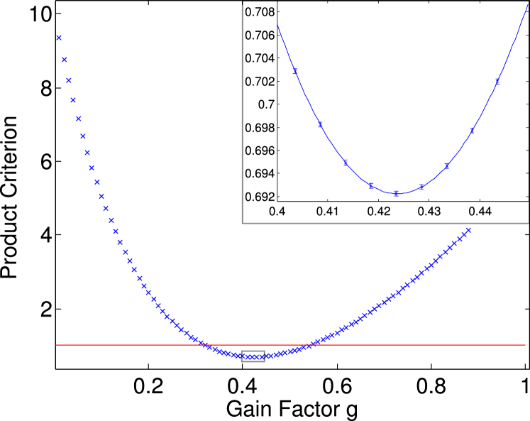
Figure 3: Entanglement distributed between modes $A^{\prime}$ and $B^{\prime}$. The experimental values for the criterion (2) are depicted in dependence of the gain factor $g$. Because of the attenuation of mode $B$ by 50 %, a gain factor of about 0.5 yields a value smaller than 1, i.e., below the limit for entanglement (solid red line). The inset zooms into the interesting section around the minimum. The depicted estimated errors are so small because of the large amount of data taken.

Discussion

The performance of the protocol can be explained using the structure of the displacements (Protocol.). Entanglement distribution without sending entanglement highlights vividly the important role played by classical information in quantum information protocols. Classical information lies in our knowledge about all the correlated displacement involved. This allows the communicating parties (or David on their behalf) to adjust the displacements locally to recover through clever noise addition quantum resources initially present in the input quantum squeezed states. Mode $C^{\prime}$ transmitted from Alice to Bob carries on top of the sub-shot-noise quadrature of the input squeezed state the displacement noise which is anticorrelated with the displacement noise of Bob’s mode. Therefore, when the modes are interfered on Bob’s beam splitter, this noise partially cancels out in the output mode $B^{\prime}$ when the light quadratures of both modes add. Moreover, the residual noise in Bob’s position (momentum) quadrature is correlated (anticorrelated) with the displacement noise in Alice’s position (momentum) quadrature in mode $A^{\prime}$, again initially squeezed. Because of this, the product of variances in criterion (2) drops below the value for separable states, and thus entanglement between Alice and Bob’s modes emerges. The difference between the theoretically proposed protocol Mista_09 and the experimental demonstration reported in this Letter lies merely in the way classical information is used. In the original protocol, the classical information is retained by David and he is responsible for clever tailoring of correlated noise. Bob evokes the required noise cancellation by carrying out the final part of the global operation via superimposing his mode with the ancilla on BS_BC. In the experimentally implemented protocol, David shares part of his information with Bob, giving Bob a possibility to get entanglement a posteriori, by using his part of the classical information after the quantum operation is carried out. Thus entanglement distribution in our case is truly performed via a dual classical and quantum channel, via classical information exchange in combination with the transmission of separable quantum states.

There are other interesting aspects to this protocol, which may open new, promising avenues for research. Noise introduced into the initial states by displacements contains specific classical correlations. On a more fundamental level, these displacements can be seen as correlated dissipation (including mode $C$ into the “environment”). It is already known that dissipation to a common reservoir can even lead to the creation of entanglement dissipation ; dissipation2 . Our scheme can be viewed as another manifestation of a positive role dissipation may play in quantum protocols.

The presence of correlated noise results in nonzero Gaussian discord at all stages of the protocol, a more general form of quantum correlations, which are beyond entanglement Adesso_10 . The role of discord in entanglement distribution has recently been discussed theoretically Streltsov_12 ; Chuan_12 . The requirements devised there are reflected in the particular separability properties of our global state after the interaction of modes $A$ and $C$ on Alice’s beam splitter. The state $\hat{\rho}_{A^{\prime}BC^{\prime}}$ contains discord and entanglement across $A^{\prime}|BC^{\prime}$ splitting and is separable and discordant across $C^{\prime}|A^{\prime}B$ splitting as required by the protocol. Our work thus illustrates an interplay of entanglement and other quantum correlations, such as correlations described by discord, across different partitions of a multipartite quantum system.

L. M. acknowledges Project No. P205/12/0694 of GAČR. N. K. is grateful for the support provided by the A. von Humboldt Foundation. The project was supported by the BMBF Grant “QuORep” and by the FP7 Project QESSENCE. We thank Christoffer Wittmann and Christian Gabriel for fruitful discussions. C. P. and V. C. contributed equally to this work.

Note added.

Recently, an experiment has been presented in Ref. Vollmer13 , which is based on a similar protocol. The main difference consists in the fact that it starts with entanglement which is hidden and recovered with thermal states. For this implementation no knowledge about classical information has to be communicated to Bob, besides the used thermal state. By contrast the setup presented in this work exhibits entanglement only at the last step of the protocol. Thus both works give good insights on different aspects of the theoretically proposed protocol Mista_09 . Another independent demonstration of a similar protocol based on discrete variables was recently presented in Ref Fedrizzi13 .

Appendix A Preparation of polarization squeezed states

To prepare two identically, polarization squeezed modes we use a well known technique like in Heersink_05 ; Leuchs99 ; Silberhorn01 ; Dong_07 . Each of these modes is generated by launching two orthogonally polarized femtosecond pulses ($\sim$200 fs) with balanced powers onto the two birefringent axes of a polarization maintaining fiber (FS-PM-7811, Thorlabs, 13 m). The pump source is a soliton-laser emitting light at a center wavelength of 1559 nm and a repetition rate of 80 MHz. By exploiting the optical Kerr effect of the fibers, the orthogonally polarized pulses are individually quadrature squeezed and subsequently temporally overlapped with a relative phase of $\pi/2$, resulting in a circular polarized light beam. The relative phase is actively controlled using an interferometric birefringence compensator including a piezoelectric transducer and a locking loop based on a 0.1 % tap-off signal after the fiber. In terms of Stokes observables (see Heersink_05 ; Korolkova_02 ) this results in states with zero mean values of $\hat{S}_{1}$ and $\hat{S}_{2}$, but a bright $\langle\hat{S}_{3}\rangle\gg 0$ component. These states exhibit polarization squeezing at a particular angle in the $\hat{S}_{1}$-$\hat{S}_{2}$-plane.

Appendix B Gaussian states

We implement the entanglement distribution protocol using optical modes which are systems in infinitely-dimensional Hilbert state space. An $N$-mode system can be conveniently characterized by the quadrature operators $\hat{x}_{j},\hat{p}_{k}$, $j,k=1,2,\ldots,N$ satisfying the canonical commutation rules $[\hat{x}_{j},\hat{p}_{k}]=i\delta_{jk}$ which can be expressed in the compact form as

$$[\hat{\xi}_{j},\hat{\xi}_{k}]=i{\Omega_{N}}_{jk}.$$ (8)

Here we have introduced the vector of quadratures $\hat{\xi}=(\hat{x}_{1},\hat{p}_{1},\ldots,\hat{x}_{N},\hat{p}_{N})$ and

$$\Omega_{N}=\bigoplus_{i=1}^{N}J,\quad J=\left(\begin{array}[]{cc}0&1\\ -1&0\\ \end{array}\right),$$ (11)

is the symplectic matrix.

The present protocol relies on Gaussian quantum states. As any standard Gaussian distribution, a Gaussian state $\hat{\rho}$ is fully characterized by the vector of its first moments

$$d=\mbox{Tr}\left(\hat{\rho}\hat{\xi}\right),$$ (12)

and by the covariance matrix $\gamma$ with elements

$$\gamma_{jk}=\mbox{Tr}[\hat{\rho}\{\hat{\xi}_{j}-d_{j}\openone,\hat{\xi}_{k}-d_{k}\openone\}],$$ (13)

where $\{\hat{A},\hat{B}\}=\hat{A}\hat{B}+\hat{B}\hat{A}$ is the anticommutator. A real symmetric positive-definite $2N\times 2N$ matrix $\gamma$ describes a covariance matrix of a physical quantum state if and only if it satisfies the condition Simon_94 :

$$\gamma+i\Omega_{N}\geq 0.$$ (14)

The separability of Gaussian states can be tested using the positive partial transpose (PPT) criterion. A single mode $j$ is separable from the remaining $N-1$ modes if and only if the Gaussian state $\hat{\rho}$ has a positive partial transposition $\hat{\rho}^{T_{j}}$ with respect to the mode $j$ Simon_00 ; Werner_01 . On the level of the covariance matrices, the partial transposition is represented by a matrix $\Lambda_{j}=\left(\bigoplus_{i\neq j=1}^{N-1}\openone^{(i)}\right)\oplus\sigma_{z}^{(j)}$, where $\sigma_{z}^{(j)}=\mbox{diag}(1,-1)$ is the diagonal Pauli $z$-matrix of mode $j$ and $\openone^{(i)}$ is the $2\times 2$ identity matrix. The matrix $\gamma^{(T_{j})}$ corresponding to a partially transposed state $\hat{\rho}^{T_{j}}$ reads $\gamma^{(T_{j})}=\Lambda_{j}\gamma\Lambda_{j}^{T}$. In terms of the covariance matrix, one can then express the PPT criterion in the following form. A mode $j$ is separable from the remaining $N-1$ modes if and only if Simon_00 ; Werner_01

$$\gamma^{(T_{j})}+i\Omega_{N}\geq 0.$$ (15)

The PPT criterion (15) is a sufficient condition for separability only under the assumption of Gaussianity. In our experiment, however, non-Gaussian states can be generated for which this criterion represents only a necessary condition for separability. Therefore it can fail in detecting entanglement.

Appendix C Analysis of non-Gaussianity

There are two sources of imperfections in our experimental set up that are potential sources of non-Gaussianity. These are phase fluctuations and the modulation of the initial squeezed states before the first beam splitter. They are discussed in the following sections.

C.1 Phase fluctuations

The experiment includes an interference of the modes $A$ and $C$ on a beam splitter, which is the first beam splitter $BS_{AC}$ in the protocol. Imperfect phase locking at this beam splitter might cause a phase drift resulting in a non-Gaussian character of the state $\hat{\rho}_{A^{\prime}C^{\prime}}$ after the beam splitter. The phase fluctuations can be modelled by a random phase shift of mode $A$ before the beam splitter described by a Gaussian distribution $P(\phi)$ with zero mean and variance $\sigma^{2}$. Denoting the operator corresponding to a beam splitter transformation as $\hat{\mathcal{U}}$ and the phase shift $\phi$ on mode $A$ as $\hat{V}_{A}(\phi)$, the state $\hat{\rho}_{A^{\prime}C^{\prime}}$ can be linked to the state $\hat{\rho}_{AC}$ before the onset of phase fluctuations as

$$\hat{\rho}_{A^{\prime}C^{\prime}}=\int_{-\infty}^{\infty}P(\phi)\hat{\mathcal{U}}\hat{V}_{A}(\phi)\hat{\rho}_{AC}\hat{V}_{A}^{{\dagger}}(\phi)\hat{\mathcal{U}}^{{\dagger}}d\phi.$$ (16)

Hence we can express the measured covariance matrix $\gamma_{A^{\prime}C^{\prime}}$ given in Eq. (3) of the main letter, and the vector of the first moments $d^{\prime}$ of the state $\hat{\rho}_{A^{\prime}C^{\prime}}$ in terms of the covariance matrix $\gamma_{AC}$ and the vector of the first moments $d$ of the input state $\hat{\rho}_{AC}$. For this it is convenient to define matrices $D$ and $D^{\prime}$ of the first moments with elements $D_{ij}=d_{i}d_{j}$ and $D^{\prime}_{ij}=d_{i}^{\prime}d_{j}^{\prime}$, $i,j=1,\ldots,4$. Using Eq. (16) and after some algebra, one gets the transformation rule for the matrix of the first moments in the form $D^{\prime}=U\Sigma D\Sigma U^{T}$, where $U$ describes the beam splitter on the level of covariance matrices. $\Sigma=\mbox{diag}(e^{-\frac{\sigma^{2}}{2}},e^{-\frac{\sigma^{2}}{2}},1,1)$ is a diagonal matrix. Similarly we get the covariance matrix

$$\gamma_{A^{\prime}C^{\prime}}=U\left(\Sigma\gamma_{AC}\Sigma+\pi\oplus 0\right)U^{T},$$ (17)

where $0$ is the $2\times 2$ zero matrix and

$$\pi=\frac{(1-e^{-\sigma^{2}})^{2}}{2}(A+\alpha)+\frac{1-e^{-2\sigma^{2}}}{2}J(A+\alpha)J^{T}.$$ (18)

Here the matrix $A$ is the $2\times 2$ matrix with elements $A_{ij}=(\gamma_{AC})_{ij}$, $i,j=1,2$, $\alpha$ is the $2\times 2$ matrix with elements $\alpha_{ij}=2D_{ij}$, $i,j=1,2$, and $J$ is defined in Eq. (11). Similar to Ref. Vollmer13 we can now invert the relation (17) and express the input covariance matrix $\gamma_{AC}$ via the output covariance matrix $\gamma_{A^{\prime}C^{\prime}}$ and the first moments after the beam splitter $BS_{AC}$ as

$$\gamma_{AC}=\Sigma^{-1}U^{T}\gamma_{A^{\prime}C^{\prime}}U\Sigma^{-1}+\tilde{\pi}\oplus 0,$$ (19)

where

$$\tilde{\pi}=\frac{(1-e^{\sigma^{2}})^{2}}{2}(\tilde{A}+\tilde{\alpha})+\frac{1-e^{2\sigma^{2}}}{2}J(\tilde{A}+\tilde{\alpha})J^{T}.$$ (20)

The $2\times 2$ matrices $\tilde{A}$ and $\tilde{\alpha}$ possess the elements $\tilde{A}_{ij}=(U^{T}\gamma_{A^{\prime}C^{\prime}}U)_{ij}$ and $\tilde{\alpha}_{ij}=2(U^{T}D^{\prime}U)_{ij}$, $i,j=1,2$.

Our estimate for the variance of the phase fluctuations is $\sigma^{2}=0.02^{\circ}$ and the vector $d^{\prime}$ of the measured mean values of the state $\hat{\rho}_{A^{\prime}C^{\prime}}$ reads

$$d^{\prime}=(-0.208,9.876,13.32,1.78).$$ (21)

By substituting these experimental values for $\sigma^{2}$ and $d^{\prime}$ in Eq. (19) and using the beam splitter with the measured transmissivity $T=0.49$ we get a legitimate covariance matrix $\gamma_{AC}$ before the phase fluctuations as can be easily verified by checking the condition (14).

Provided that the state with the covariance matrix $\gamma_{AC}$ is classical it can be expressed as a convex mixture of products of coherent states. Gaussian distributed phase fluctuations and a beam splitter preserve the structure of the state, hence the state after the first beam splitter cannot be entangled. The covariance matrix $\gamma_{AC}$ determines a physical Gaussian quantum state. Moreover, the covariance matrix possesses all eigenvalues greater than one and therefore the state is not squeezed Simon_94 which is in a full agreement with the fact that modulations of modes $A$ and $C$ completely destroy the squeezing. It then follows that this Gaussian state is classical and it therefore transforms to a separable state after the first beam splitter.

The inversion (19) thus allows us to associate a Gaussian state before the phase fluctuations with the covariance matrix $\gamma_{A^{\prime}C^{\prime}}$ measured after the first beam splitter. The separability properties of the state after the beam splitter can then be determined from the non-classicality properties of this Gaussian state.

C.2 Gaussianity of the utilized states

We have paid great attention on the modulations on modes $A$ and $C$ to preserve Gaussian character of the state $\hat{\rho}_{A^{\prime}C^{\prime}}$. Our success can be visually inspected at the examples in Fig. 4, which illustrates that both the modulation and the subsequent Gaussian mixing faithfully samples the required Gaussian shape.

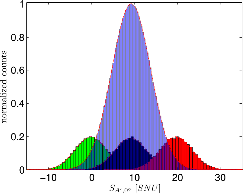
Figure 4: Histogram plots for $\hat{S}_{A^{\prime},0^{\circ}}$ of the Gaussian mixed state (blue) and three exemplary individual modes. This figure illustrates the preparation of the Gaussian mixed state via post processing. Exemplarily, three of the 6400 displaced individual modes are visualized by their histograms (in green, black and red colour). The normalization is chosen such that they can be depicted in the same plot as the histogram of the mixed state (blue), which is normalized to its maximum value. By merging the data for all individual modes using a weighting with a two dimensional Gaussian distribution, the mixed state is achieved. Its Gaussianity is visualized by the Gaussian fit (red curve).

Besides this raw visual check we have also tested quantitatively Gaussianity of the involved states by measuring higher-order moments of the Stokes measurements on modes $A^{\prime}$ and $C^{\prime}$. Specifically, we have focused on the determination of the shape measures called skewness $S$ and kurtosis $K$ defined for a random variable $x$ as the following third and fourth standardized moments

$$S=\frac{\mu_{3}}{s^{3}},\quad K=\frac{\mu_{4}}{s^{4}},$$ (22)

where $\mu_{k}=\langle(x-\langle x\rangle)^{k}\rangle$ is the $k$th central moment, $\langle x\rangle$ is the mean value and $s=\sqrt{\mu_{2}}$ is the standard deviation.

Skewness characterizes the orientation and the amount of skew of a given distribution and therefore informs us about its asymmetry in the horizontal direction. Gaussian distributions possess skewness of zero. The exemplary values of skewness for various measurement settings are summarized in the Table 2.

Table 1: Skewness $S$ for Stokes measurements on modes $A^{\prime}$ and $C^{\prime}$ in different measurement directions.

Measurement	$S_{A^{\prime},0^{\circ}}$	$S_{A^{\prime},90^{\circ}}$
Skewness$\times 10^{3}$	$6.240\pm 0.781$	$-1.478\pm 0.563$
Measurement	$S_{C^{\prime},0^{\circ}}$	$S_{C^{\prime},90^{\circ}}$
Skewness$\times 10^{3}$	$10.123\pm 0.727$	$1.106\pm 0.830$

Table 2: Kurtosis $K$ for Stokes measurements on modes $A^{\prime}$ and $C^{\prime}$ in different measurement directions.

Measurement	$S_{A^{\prime},0^{\circ}}$	$S_{A^{\prime},90^{\circ}}$
Kurtosis	$2.971\pm 2.211\times 10^{-3}$	$2.986\pm 1.852\times 10^{-3}$
Measurement	$S_{C^{\prime},0^{\circ}}$	$S_{C^{\prime},90^{\circ}}$
Kurtosis	$2.972\pm 1.978\times 10^{-3}$	$2.992\pm 1.568\times 10^{-3}$

The skewness can vanish also for the other symmetrical distributions, which may, however, differ from a Gaussian distribution in the peak profile and the weight of tails. These differences can be captured by the kurtosis which is equal to 3 for Gaussian distributions. The exemplary values of kurtosis for various measurement settings are summarized in the Table 2.

The tables reveal that the measured probability distributions satisfy within the experimental error the necessary Gaussianity conditions $S=0$ and $K=3$. More sophisticated normality tests can be performed, which is beyond the scope of the present manuscript.

Appendix D Statistical errors of the measured covariance matrices

By dividing our dataset in 10 equal in size parts we can estimate the statistical errors of our measured covariance matrices $\gamma_{A^{\prime}C^{\prime}}$ and $\gamma_{A^{\prime}B^{\prime}}$ given in Eqs. (3) and (5) of the main letter. We calculate the covariance matrix for each part and use the standard deviation as error estimation. The covariance matrix $\gamma_{A^{\prime}C^{\prime}}$ including the statistical error turns out to be

$$\gamma_{A^{\prime}C^{\prime}}=\begin{pmatrix}20.90\pm 0.0087&1.102\pm 0.0091&-7.796\pm 0.0069&-1.679\pm 0.0076\\ 1.102\pm 0.0091&25.30\pm 0.013&1.000\pm 0.0071&14.63\pm 0.0091\\ -7.796\pm 0.0069&1.000\pm 0.0071&20.68\pm 0.0093&0.8010\pm 0.011\\ -1.679\pm 0.0076&14.63\pm 0.0091&0.8010\pm 0.011&24.65\pm 0.0073\end{pmatrix}.$$ (23)

Similarly, the covariance matrix $\gamma_{A^{\prime}B^{\prime}}$ including the statistical error reads as

$$\gamma_{A^{\prime}B^{\prime}}=\begin{pmatrix}19.95\pm 0.011&1.025\pm 0.016&-4.758\pm 0.0050&-1.063\pm 0.0051\\ 1.025\pm 0.016&22.92\pm 0.012&0.9699\pm 0.0047&9.153\pm 0.0058\\ -4.758\pm 0.0050&0.9699\pm 0.0047&9.925\pm 0.0048&0.2881\pm 0.0047\\ -1.063\pm 0.0051&9.153\pm 0.0058&0.2881\pm 0.0047&11.65\pm 0.0038\end{pmatrix}.$$ (24)

We could achieve such small statistical errors by recording sufficient large datasets.

References

- (1) E. Schrödinger, Naturwissenschaften 23, 807 (1935).
- (2) A. Einstein, B. Podolsky, and N. Rosen, Phys. Rev. 47, 777 (1935).
- (3) M. D. Reid, Phys. Rev. A 40, 913 (1989).
- (4) H. M. Wiseman, S. J. Jones, and A. C. Doherty, Phys. Rev. Lett. 98, 140402 (2007).
- (5) J. S. Bell, Physics (Long Island City, N.Y.) 1, 195 (1965).
- (6) N. J. Cerf and C. Adami, Phys. Rev. Lett. 79, 5194 (1997).
- (7) M. Horodecki, J. Oppenheim, and A. Winter, Nature (London) 436, 673 (2005).
- (8) C. H. Bennett, G. Brassard, C. Crépeau, R. Jozsa, A. Peres, and W. K. Wootters, Phys. Rev. Lett. 70, 1895 (1993).
- (9) M. Žukowski, A. Zeilinger, M. A. Horne, and A. K. Ekert, Phys. Rev. Lett. 71, 4287 (1993).
- (10) H.-J. Briegel, W. Dür, J. I. Cirac, and P. Zoller, Phys. Rev. Lett. 81, 5932 (1998).
- (11) A. K. Ekert, Phys. Rev. Lett. 67, 661 (1991).
- (12) C. H. Bennett and S. J. Wiesner, Phys. Rev. Lett. 69, 2881 (1992).
- (13) R. Raussendorf and H.-J. Briegel, Phys. Rev. Lett. 86, 5188 (2001).
- (14) J.-W. Pan, D. Bouwmeester, H. Weinfurter, and A. Zeilinger, Phys. Rev. Lett. 80, 3891 (1998).
- (15) T. S. Cubitt, F. Verstraete, W. Dur and J. I. Cirac, Phys. Rev. Lett. 91, 037902 (2003).
- (16) A. Streltsov, H. Kampermann, and D. Bruß, Phys. Rev. Lett. 108, 250501 (2012).
- (17) T. K. Chuan, J. Maillard, K. Modi, T. Paterek, M. Paternostro, and M. Piani, Phys. Rev. Lett. 109, 070501 (2012).
- (18) A. Kay, Phys. Rev. Lett. 109, 080503 (2012).
- (19) L. Mišta, Jr. and N. Korolkova, Phys. Rev. A 80, 032310 (2009).
- (20) L. Mišta, Jr. and N. Korolkova, Phys. Rev. A 86, 040305 (2012).
- (21) A. Peres, Phys. Rev. Lett. 77, 1413 (1996).
- (22) M. Horodecki, P. Horodecki, and R. Horodecki, Phys. Lett. A 223, 1 (1996).
- (23) R. F. Werner and M. M. Wolf, Phys. Rev. Lett. 86, 3658 (2001).
- (24) V. Giovannetti, S. Mancini, D. Vitali, and P. Tombesi, Phys. Rev. A 67, 022320 (2003).
- (25) R. Dong, J. Heersink, J.-I. Yoshikawa, O. Glöckl, U. L. Andersen, and G. Leuchs, New J. Phys. 9, 410 (2007).
- (26) J. Heersink, V. Josse, G. Leuchs, and U. L. Andersen, Opt. Lett. 30, 1192 (2005).
- (27) N. Korolkova, G. Leuchs, R. Loudon, T. C. Ralph, and C. Silberhorn, Phys. Rev. A 65, 052306 (2002).
- (28) G. Leuchs, T. C. Ralph, C. Silberhorn, and N. Korolkova, J. Mod.Opt. 46, 1927 (1999).
- (29) C. Silberhorn, P. K. Lam, O. Weiß, F. König, N. Korolkova, and G. Leuchs, Phys. Rev. Lett. 86 4267 (2001).
- (30) F. Benatti and R. Floreanini, J. Phys. A 39, 2689 (2006).
- (31) D. Mogilevtsev, T. Tyc and N. Korolkova, Phys. Rev. A 79, 053832 (2009).
- (32) G. Adesso and A. Datta, Phys. Rev. Lett. 105, 030501 (2010).
- (33) C. E. Vollmer, D. Schulze, T. Eberle, V. Händchen, J. Fiurášek, and R. Schnabel, arXiv:1303.1082 [accepted by Phys. Rev. Lett.] (2013).
- (34) A. Fedrizzi, M. Zuppardo, G. G. Gillett, M. A. Broome, M. de Almeida, M. Paternostro, A. G. White, and T. Paterek, arXiv:1303.4634 [accepted by Phys. Rev. Lett.] (2013).
- (35) R. Simon, N. Mukunda, and B. Dutta, Phys. Rev. A 94, 1567 (1994).
- (36) R. Simon, and P. Horodecki, Phys. Rev. Lett. 84, 2726 (2000).