A state polytope decomposition formula

Abstract.

We give a decomposition formula for computing the state polytope of a reducible variety in terms of the state polytopes of its components: If a polarized projective variety $X$ is a chain of subvarieties $X_{i}$ satisfying some further conditions, then the state polytope of $X$ is the Minkowski sum of the state polytopes of $X_{i}$ translated by a vector $\tau$ which can be readily computed from the ideal of $X_{i}$. The decomposition is in the strongest sense in that the vertices of the state polytope of $X$ are precisely the sum of vertices of the state polytopes of $X_{i}$ translated by $\tau$. We also give a similar decomposition formula for the Hilbert-Mumford index of the Hilbert points of $X$. We give a few examples of the state polytope and the Hilbert-Mumford index computation of reducible curves which are interesting in the context of the log minimal model program for the moduli space of stable curves.

1. Introduction

The state polytope of an ideal encodes much information about the scheme it defines. Let $V$ be a vector space over an algebraically closed field $k$ of characteristic zero. Given a rational representation $W$ of ${\mathrm{S}L}(V)$ and a maximal torus $T\subset{\mathrm{S}L}(V)$, Kempf [Kem78, §3] defined the state of $w\in W$ (with respect to $T$) to be the set of the characters $\chi\in X(T)$ such that $w_{\chi}\neq 0$ where $w_{\chi}$ is the projection of $w$ in the weight space $W_{\chi}$. Given a projective variety $X\subset\mathbb{P}(V)$ and a choice of homogeneous coordinates, Bayer and Morrison in [BM88] defined the $m$th state polytope of $X\subset\mathbb{P}(V)$ to be the convex hull of the states of (any affine point over) the $m$th Hilbert point $[X]_{m}\in\mathbb{P}\left(\bigwedge^{Q(m)}S^{m}V^{*}\right)$ defined:

$$\left[(I_{X})_{m}\to S^{m}V^{*}\right]\in Gr_{Q(m)}S^{m}V^{*})\hookrightarrow\mathbb{P}\left(\bigwedge^{Q(m)}S^{m}V^{*}\right)$$

where $I_{X}$ is the saturated homogeneous ideal of $X$, $Q(t)$ is the dimension of the $t$th graded piece $(I_{X})_{t}$, and $m$ is a positive integer bigger than or equal to the Castelnuovo-Mumford regularity of $X$. The state polytope of a homogeneous ideal is the state polytope of the projective variety it defines. The relation between the state polytopes and the Gröbner theory is described by:

Theorem 1.1.

[BM88, Theorem 3.1]   There is a natural one-to-one correspondence between the initial ideals and the vertices of the state polytope.

Let $T$ be the maximal torus of ${\mathrm{S}L}(V^{*})$ diagonalized by $x_{0},\dots,x_{n}$. Then by considering the $T$-weight space decomposition of $\bigwedge^{Q(m)}S^{m}V^{*}$, one can naturally associate the characters in the state of a Hilbert point $\left[(I_{X})_{m}\to S^{m}V^{*}\right]$ and the monomials $x^{\alpha(1)}\wedge\cdots\wedge x^{\alpha(Q(m))}$ whose associated Plücker coordinate does not vanish at $[X]_{m}$. See [MS11] for this correspondence (Section 3.1) as well as for a very nice exposition on Kempf’s theory of the worst one-parameter subgroup and basics on state polytopes. In particular, the trivial character corresponds to the barycenter of which coordinates are all $\frac{mQ(m)}{\dim V}$.

In view of this correspondence, we take the following definition of the state polytope [Stu96, Formula (2.7)]:

Definition 1.2.

Given a homogeneous ideal $I\subset S=k[x_{0},\dots,x_{n}]$ and $m\geq\textup{reg}(I)$, the $m$th state polytope is defined and denoted by

(1) $${\mathcal{P}}_{m}(I):=\textup{Conv}\left\{\left.\sum_{x^{\alpha}\in\textup{\bf in}\,_{\prec}(I)_{m}}\alpha\,\right|\mbox{$\prec$ is a monomial order}\right\}.$$

Here, Conv means taking the convex hull and $\textup{reg}(I)$ is the Castelnuovo-Mumford regularity of $I$, and the condition $m\geq\textup{reg}(I)$ ensures that the $m$th Hilbert point of the scheme $X$ cut out by $I$ is well defined.

Apparent from the definition is that the state polytope can be computed from the universal Gröbner basis. More importantly, ${\mathcal{P}}_{m}(I_{X})$ determines the semistability of the Hilbert point $[X]_{m}$ with resect to the chosen basis. This is a direct consequence of the Mumford’s numerical criterion [Mum65]: $[X]_{m}$ is $T$-semistable (resp. $T$-stable) if and only if the state polytope in $X(T)$ (resp. interior of the polytope) contains the trivial character. This condition is equivalent to the state polytope (1) (resp. its interior) containing the barycenter, where the coordinates $x_{0},\dots,x_{n}$ are chosen so that $T$ acts on them via characters i.e. they diagonalize the $T$ action. The upshot is that, by computing the universal Gröbner basis (with a computer algebra system if and when convenient), one can determine the semistability with respect to the given coordinates i.e. with respect to the associated maximal torus $T$. If $[X]_{m}$ is $T$-unstable for some $T$, then $[X]_{m}$ is GIT unstable.

Of course, to prove the semistability of $[X]_{m}$, one has to prove its $T$-semistability for all maximal torus $T$, so in that regard the state polytope formulation of GIT semistability may not seem too much of a help. But in the special case when $X\subset\mathbb{P}(V)$ and $V$ is a multiplicity-free representation of a linearly reductive subgroup $\Gamma$ of $\textup{Aut}(X)$, the (semi)stability of $[X]_{m}$ is equivalent to the $T$-(semi)stability with respect to any maximal torus $T$ that preserves the $\Gamma$-irreducibles of $V$ [MS11, Proposition 4.7]. This is the key idea of Morrison and Swinarski that allowed them to prove the $m$-Hilbert semistability of various curves for small $m$ (§7, ibid). It was also the starting point for Alper, Fedorchuk and Smyth to obtain their results on the $m$-Hilbert semistability of canonical and bicanonical images of generic smooth curves for $m\geq 2$ [AFS10], which should prove essential in carrying out the log minimal model program for $\overline{M}_{g}$ (the Hassett-Keel program). In fact, Alper, Fedorchuk and Smyth do not rely on the state polytope technique: Instead, they work out by hand a collection of basis members for the (bi)canonical system and deduce from them the semistability directly, which is in every manner very impressive.

Inspired from the exciting developments, we shall consider in this article how one can more efficiently compute the state polytope of certain reducible varieties. More precisely, we give a formula for the state polytope of a variety in terms of the state polytopes of its subvarieties. We say that $X$ is a chain of subvarieties $X_{i}$ if $X=\cup_{i=1}^{\ell}X_{i}$ and $X_{i}$ meets $X_{j}$ when and only when $|i-j|=1$.

Theorem 1.3.

Let $X$ be a chain of subvarieties $X_{1},\dots,X_{\ell}$ defined by a homogeneous ideal $I_{X}=\cap_{i}I_{X_{i}}$. Suppose that there is a homogeneous coordinate system $x_{0},\dots,x_{n}$ and a sequence $n_{0}=0<n_{1}<\cdots<n_{\ell}=n$ such that

$$X_{i}\subset\{x_{0}=\cdots=x_{n_{i-1}-1}=0,x_{n_{i}+1}=x_{n_{i}+2}=\cdots=x_{n}=0\}.$$

Then the state polytope of $X$ is given by the following decomposition formula

($$\dagger {\mathcal{P}}_{m}(I_{X})=\sum_{i=1}^{\ell}{\mathcal{P}}_{m}(I_{X_{i}}\cap k[x_{n_{i-1}},\cdots,x_{n_{i}}])+\sum_{i=1}^{\ell-1}{\mathcal{P}}_{m}(T_{i}\cap k[x_{n_{i-1}},\dots,x_{n}])$$)

where $T_{i}=\langle x_{n_{i-2}},\dots,x_{n_{i-1}-1}\rangle\langle x_{n_{i}+1},\dots,x_{n}\rangle$ for $2\leq i\leq\ell-1$, and $T_{1}=\langle x_{n_{1}+1},x_{n_{1}+2},\dots,x_{n}\rangle$ and $T_{\ell}=\langle x_{n_{\ell-2}},x_{n_{\ell-2}+1},\dots,x_{n_{\ell-1}-1}\rangle$.

Remark 1.4.

1. Here, ${\mathcal{P}}_{m}(I_{X_{i}}\cap k[x_{n_{i-1}},\cdots,x_{n_{i}}])$ is regarded as a convex polytope in the subspace

   $$\{(a_{0},\dots,a_{n})\in\mathbb{R}^{n+1}\,|\,a_{0}=\cdots=a_{n_{i-1}-1}=0,a_{n_{i}+1}=a_{n_{i}+2}=\cdots=a_{n}=0\}.$$

   Similarly, ${\mathcal{P}}_{m}(T_{i}\cap k[x_{n_{i-1}},\dots,x_{n}])$ is also regarded as a convex polytope in the relevant vector subspace.

2. Note that the second term of ($\dagger$ ‣ 1.3) is zero dimensional since $T_{i}$ are monomial ideals. We shall reserve the letter $\tau$ to denote it.

In fact, the polytope decomposition in Theorem 1.3 is sharp in the following sense:

Corollary 1.5.

Retain notations from Theorem 1.3. Let $\mathcal{V}_{i}$ denote the set of vertices of ${\mathcal{P}}_{m}(I_{X_{i}}\cap k[x_{n_{i-1}},\dots,x_{n_{i}}])$, $i=1,\dots,\ell$. Then the vertices of ${\mathcal{P}}_{m}(I_{X})$ are precisely

$$\left\{\left.\tau+\sum_{i=1}^{\ell}v_{i}\,\right|\,v_{i}\in\mathcal{V}_{i}\right\}.$$

The Hilbert-Mumford index can also be computed by a similar decomposition formula. To be consistent with our main reference [HHL10], we state the formula in terms of the dual Hilbert point

$$[X]_{m}^{\star}=[S^{m}V^{*}\to S^{m}V^{*}/I_{m}]\in Gr^{P(m)}S^{m}V^{*}\hookrightarrow\mathbb{P}\left(\bigwedge^{P(m)}S^{m}V^{*}\right).$$

where $P(t)\in\mathbb{Q}[t]$ is the Hilbert polynomial of $X$.

Proposition 1.6.

Let $X$ be as in Theorem 1.3 and $\rho:\mathbb{G}_{m}\to{\mathrm{G}L}_{n+1}$ be a 1-parameter subgroup of ${\mathrm{G}L}_{n+1}$ diagonalized by $\{x_{0},\dots,x_{n}\}$ with weights $(r_{0},\cdots,r_{n})$ and $\rho_{i}$ be the restriction of $\rho$ to ${\mathrm{G}L}(kx_{n_{i-1}}+\cdots+kx_{n_{i}})$. Then the Hilbert-Mumford index $\mu([X]_{m}^{\star},\rho)$ of the $m$th Hilbert point of $X$ with respect to $\rho$ is given by

$$\mu([X]_{m}^{\star},\rho)=\sum_{i=1}^{\ell}\mu([X_{i}]_{m}^{\star},\rho_{i})-\sum_{i=1}^{\ell}\bigg{(}\frac{mP_{i}(m)}{n_{i}-n_{i-1}+1}\sum_{k=n_{i-1}}^{n_{i}}r_{k}\bigg{)}+\frac{mP(m)}{n+1}\sum_{i=0}^{n}r_{i}+m\sum_{i=1}^{\ell-1}r_{n_{i}}$$

where $P(m)$ is the Hilbert polynomial of $I_{X}\subset k[x_{0},\dots,x_{n}]$ and $P_{i}(m)$, the Hilbert polynomial of $I_{X_{i}}\cap k[x_{n_{i-1}},\dots,x_{n_{i}}]$ regarded as an ideal in $k[x_{n_{i-1}},\dots,x_{n_{i}}]$.

We shall give proofs of Theorem 1.3 and Proposition 1.6 in §4. Corollary 1.5 will be established in §3.

2. Basic examples

Before proving the main results, we shall give a few basic examples at the far ends of the spectrum, namely, monomial ideals and hypersurfaces (plane curves, to be more specific).

Example 2.1 (Monomial ideals).

Let $X=X_{1}\cup X_{2}\cup X_{3}\subset\mathbb{P}^{3}$ be a chain of $\mathbb{P}^{1}$’s:

$$X_{1}=\{x_{2}=x_{3}=0\},\quad X_{2}=\{x_{0}=x_{3}=0\},\quad X_{3}=\{x_{0}=x_{1}=0\}.$$

Then $I_{X_{1}}\cap k[x_{0},x_{1}]=0$ and it does not contribute to the state polytope. The other components do not contribute for the same reason, but the mixed terms

$$\{x_{0}x_{2},x_{0}x_{3}\}\cup\{x_{0}x_{3},x_{1}x_{3}\}$$

are precisely the monomial generators of the ideal of $X$, and the formula ($\dagger$ ‣ 1.3) holds.

More generally, if $X=\cup X_{i}$ as in Theorem 1.3 and each $X_{i}$ are defined by monomials $M_{i\alpha}$,

$${\mathcal{P}}_{m}(I_{X_{i}}\cap k[x_{n_{i-1}},\dots,x_{n_{i}}])=\left\{\sum_{\alpha}\log_{x}M_{i\alpha}\right\}$$

where $\log_{x}x^{\alpha}=\alpha$. The formula ($\dagger$ ‣ 1.3) implies that

$${\mathcal{P}}_{m}(I_{X})=\left\{\sum_{i}\sum_{\alpha}\log_{x}M_{i\alpha}+\sum_{x^{\beta}\in\sum_{i}T_{i}}\beta\right\}.$$

This is the same as

$${\mathcal{P}}_{m}(I_{X})=\left\{\sum_{x^{\alpha}\in(I_{X})_{m}}\alpha\right\}$$

since

$$I_{X}=\cap_{i}I_{X_{i}}=\cap_{i}\langle\{M_{i\alpha}\}_{\alpha},x_{0},\dots,x_{n_{i-1}-1},x_{n_{i}+1},\dots,x_{n}\rangle=\langle\{M_{i\alpha}\}_{i,\alpha}\rangle+\sum_{i}T_{i}.$$

Note that the inclusion $M_{i\alpha}\in\cap_{i}I_{X_{i}}$ follows from the assumption that $M_{i\alpha}$ is not a power of $x_{n_{i}}$ or of $x_{n_{i-1}}$.

Example 2.2 (Plane curves).

We consider a simple example of two plane curves

$$E_{1}=\{b^{2}c=a(a-c)(a-2c),d=e=0\}\quad\mbox{and}\quad E_{2}=\{d^{2}c=e^{2}(e+c),a=b=0\}$$

meeting in one node. Let $C$ denote the union of $E_{1}$ and $E_{2}$. The $3$rd state polytope of $E_{1}$ has three vertices

(2) $$\{(3,0,0,0,0),(1,0,2,0,0),(0,2,1,0,0)\}$$

and that of $E_{2}$ has two vertices

(3) $$\{(0,0,1,2,0),(0,0,0,0,3)\}.$$

Indeed, since $E_{i}$ are hypersurfaces (in suitable linear subspaces) of degree three, their 3rd state polytopes are precisely the Newton polytopes.

To compute the state polytope of $C$, we first take the sums of a point from $(\ref{E:E1})$ and a point from $(\ref{E:E2})$:

$$\{(3,0,1,2,0),(3,0,0,0,3),(1,0,3,2,0),(1,0,2,0,3),(0,2,2,2,0),(0,2,1,0,3)\}.$$

By the decomposition formula, the vertices themselves are these translated by $\tau$ which is the sum of the exponent vectors of

$$T=\{a^{2}d,abd,acd,ad^{2},ade,a^{2}e,abe,ace,ae^{2},b^{2}d,bcd,bd^{2},bde,b^{2}e,bce,be^{2}\}.$$

We compute $\tau=(11,11,4,11,11)$, and hence the vertices of ${\mathcal{P}}_{3}(I_{C})$ are:

$$\begin{array}[]{c}(14,11,5,13,11),(14,11,4,11,14),(12,11,7,13,11),\\ (12,11,6,11,14),(11,13,6,13,11),(11,13,5,11,14).\end{array}$$

This agrees with the direct computation of the $3$rd state polytope of the ideal of $C$:

$$\langle be,ae,bd,ad,-cd^{2}+e^{3}+e^{2},a^{3}-3a^{2}c-b^{2}c+2ac^{2}\rangle$$

Here we demonstrate the output of the Macaulay 2 [GS] package StatePolytope written by D. Swinarski.

i2 : R = QQ[a,b,c,d,e];
i3 : I1 = ideal(b^2*c - a*(a-c)*(a-2*c))
              3     2     2        2
o3 = ideal(- a  + 3a c + b c - 2a*c )
o3 : Ideal of R
i4 : I2 = ideal(d^2*c-e^2*(e+1))
              2    3    2
o4 = ideal(c*d  - e  - e )
o4 : Ideal of R
i5 : I = intersect(I1+ideal(d,e),I2+ideal(a,b))
                                     2    3    2   3     2     2        2
o5 = ideal (b*e, a*e, b*d, a*d, - c*d  + e  + e , a  - 3a c - b c + 2a*c )
o5 : Ideal of R
i6 : statePolytope(3,I)
LP algorithm being used: "cddgmp".
polymake: used package cddlib
  Implementation of the double description method of Motzkin et al.
  Copyright by Komei Fukuda.
  http://www.ifor.math.ethz.ch/~fukuda/cdd_home/cdd.html

VERTICES
1 14 11 5 13 11
1 14 11 4 11 14
1 12 11 6 11 14
1 11 13 5 11 14
1 12 11 7 13 11
1 11 13 6 13 11


o6 = {{14, 11, 5, 13, 11}, {14, 11, 4, 11, 14}, {12, 11, 6, 11, 14},
     ---------------------------------------------------------------
      {11, 13, 5, 11, 14}, {12, 11, 7, 13, 11}, {11, 13, 6, 13, 11}}

Example 2.3.

This example is non-trivial compared to the previous two. We shall consider a particular genus four curve with a genus two tail. Let $R$ be a rational curve with a rhamphoid cusp. It is of arithmetic genus two and admits a $\mathbb{G}_{m}$ action with two fixed points one of which is the cusp. The action comes from the automorphism of its normalization. Let $C$ be a genus two curve obtained by attaching two copies $R_{1},R_{2}$ of $R$ at the smooth fixed points, say $p_{i}\in R_{i}$, $i=1,2$.

2pt $R_{1}$ at 85 625 $y^{2}=x^{5}$ at 136 685 $p$ at 215 635 $R_{2}$ at 350 625

Figure 1.

We bicanonically embed $C$ in $\mathbb{P}^{8}$ and consider its state polytope. Note that $R_{1}$ can be parametrized by

$$\begin{array}[]{lll}\mathbb{P}^{1}&\rightarrow&\mathbb{P}^{8}\\ \left[s,t\right]&\mapsto&\left[s^{6},s^{4}t^{2},s^{2}t^{4},st^{5},t^{6},{\bf 0}_{4}\right]\end{array}$$

which has a rhamphoid cusp at $[1,0,\dots,0]$ and $p:=[{\bf 0}_{4},1,{\bf 0}_{4}]$ is fixed under the automorphism where ${\bf 0}_{i}=(\underbrace{0,\dots,0}_{i})$. $R_{2}$ is parametrized similarly, from which we can compute its defining saturated ideal. The $6$th state polytope of $I_{R_{1}}\cap k[x_{0},\dots,x_{4}]$ has $51$ vertices

$$\{(216,191,206,206,231,{\bf 0}_{4}),(216,191,191,236,216,{\bf 0}_{4}),\cdots,(181,248,210,180,231,{\bf 0}_{4})\}$$

which are obtained by Swinarski’s StatePolytope.

The state polytope of $I_{R_{2}}\cap k[x_{4},\dots,x_{8}]$ is the mirror flip of the above with respect to $x_{4}$. By the decomposition formula, the $6$th state polytope $P$ of $C$ is $\tau$-translate of the convex hull of $51\cdot 51=2601$ vertices obtained by choosing one from each state polytope and adding them up. Being the state polytope of a product of ideals of linear subspaces, $\tau$ can be readily computed either by hand or a computer algebra system:

$$\tau=(1750,1750,1750,1750,1504,1750,1750,1750,1750).$$

The barycenter of this state polytope is $v=(1956,1956,\dots,1956)$. How can we utilize the decomposition formula to check whether $v$ is in the state polytope? A natural thing to do is to try to decompose $v-\tau$ into the two symmetric points $v_{1}=(206,206,206,206,226,{\bf 0}_{4})$ and $v_{2}=({\bf 0}_{4},226,206,206,206,206)$, and see if $v_{i}$ is contained in $6$th state polytope of $R_{i}$. But this can be easily checked by using the function contains of the polyhedra package in Macaulay 2 as follows.

i3 : R=QQ[a,b,c,d,e];
i4 : Q=QQ[s,t];
i5 : f=map(Q,R,{s^6,s^4*t^2,s^2*t^4,s*t^5,t^6});
o5 : RingMap Q <--- R
i6 : I=ker f;
o6 : Ideal of R
i7 : L=statePolytope(6,I);
i8 : P1=convexHull transpose matrix L;
i9 : v1=transpose matrix {{206,206,206,206,226}};
              5        1
o9 : Matrix ZZ  <--- ZZ
i10 : contains(P1,v1)
o10 = true

Hence, we conclude that $v$ is contained in $P$. In fact, the ideal of $C$ is simple enough so that its state polytope can be directly computed by using the state polytope package of Macaulay 2, which agrees with the result obtained above.

The assumption on the existence of the coordinate system as in Theorem 1.3 may seem quite restrictive, but we shall see that it is satisfied by an important class of varieties namely, the pluricanonical images of the generic members of the boundary of $\overline{M}_{g}$. We shall give a few interesting examples in this vein in §6.

3. Decomposition formula for initial ideals

First we shall prove a key lemma on initial ideals from which the main theorem follows with some simple observations regarding the monomial orders. Let $Y$ and $Z$ be closed subvarieties in $\mathbb{P}^{n}$ defined by homogeneous ideals $I_{Y}$ and $I_{Z}$ of $k[x_{0},\dots,x_{n}]$ respectively, and let $X$ be the projective variety defined by $I_{X}:=I_{Y}\cap I_{Z}$. Suppose that with respect to the homogeneous coordinate system $x_{0},x_{1},\cdots,x_{n}$, the subvarieties $Y$ and $Z$ are contained in linear subspaces as follows:

$$\begin{array}[]{l}Y\subset L_{1}:=\{x_{0}=\cdots=x_{l-1}=0\}\cong\mathbb{P}^{n-l}\\ Z\subset L_{2}:=\{x_{l+1}=\cdots=x_{n}=0\}\cong\mathbb{P}^{l}.\end{array}$$

In particular, $Y\cap Z=\{p\}$ where $p$ is the unique point in $L_{1}\cap L_{2}$ whose coordinates are all zero except $x_{l}$.

Lemma 3.1.

Let $\prec$ be a monomial order. The initial ideal of $I$ with respect to $\prec$ is given by

($$\dagger\dagger \textup{\bf in}\,_{\prec}(I_{X})=\langle\textup{\bf in}\,_{\prec}(I_{Y}\cap k[x_{l},\cdots,x_{n}])\rangle+\langle\textup{\bf in}\,_{\prec}(I_{Z}\cap k[x_{0},\cdots,x_{l}])\rangle+T$$)

where $T=\langle x_{0},\dots,x_{l-1}\rangle\langle x_{l+1},\dots,x_{n}\rangle$. Note that $\textup{\bf in}\,_{\prec}(I_{Y}\cap k[x_{l},\cdots,x_{n}])$ is computed as an ideal of $k[x_{l},\cdots,x_{n}]$ and $\langle\textup{\bf in}\,_{\prec}(I_{Y}\cap k[x_{l},\cdots,x_{n}])\rangle$ is the ideal in $k[x_{0},\cdots,x_{n}]$ it generates. A similar statement for $Z$ is noted.

Proof.

We first note that $T$ is contained in $\textup{\bf in}\,_{\prec}(I_{X})$ since it is a monomial ideal contained in $I_{X}$.

Let $x^{\alpha}=\prod x_{i}^{\alpha_{i}}$ be a monomial in $\textup{\bf in}\,_{\prec}(I_{X})_{m}$ i.e. $x^{\alpha}=\textup{\bf in}\,_{\prec}(f)$ for some $f\in I_{X}$. If $x^{\alpha}\notin T$, then $x^{\alpha}$ is contained in $k[x_{0},\cdots,x_{l}]$ or $k[x_{l},\cdots,x_{n}]$. If $x^{\alpha}\in k[x_{0},\cdots,x_{l}]$, then $\textup{\bf in}\,_{\prec}(g)=x^{\alpha}$ where $g(x_{0},\dots,x_{l})=f(x_{0},\cdots,x_{l},0,\cdots,0)$. But $g\in I_{Z}\cap k[x_{0},\cdots,x_{l}]$, so $x^{\alpha}$ is contained $\textup{\bf in}\,_{\prec}(I_{Z}\cap k[x_{0},\cdots,x_{l}])_{m}$. Similarly, if $x^{\alpha}\in k[x_{l},\cdots,x_{n}]$, then $x^{\alpha}\in\textup{\bf in}\,_{\prec}(I_{Y}\cap k[x_{l},\cdots,x_{n}])_{m}$. This proves that the left hand side is contained in the right.

To see the other inclusion, suppose that $x^{\alpha}\in\textup{\bf in}\,_{\prec}(I_{Y}\cap k[x_{l},\cdots,x_{n}])_{m}$ i.e., $x^{\alpha}=\textup{\bf in}\,_{\prec}(f)$ for some $f\in I_{Y}\cap k[x_{l},\cdots,x_{n}]$. Monomials of $k[x_{l},\dots,x_{n}]$ that do not vanish at $p$ are of the form $x_{l}^{i}$. But since $f$ is homogeneous and vanishes at $p\in Y$, it cannot have the term $x_{l}^{\textup{deg}\,(f)}$, so each term of $f$ is divisible by $x_{i}$ for some $i>l$. This implies that $f$ vanishes on $Z$ so that $f\in I_{X}$ and $x^{\alpha}\in\textup{\bf in}\,_{\prec}(I_{X})$. Hence $\textup{\bf in}\,_{\prec}(I_{Y}\cap k[x_{l},\cdots,x_{n}])\subset\textup{\bf in}\,_{\prec}(I_{X})$, and by a similar argument $\textup{\bf in}\,_{\prec}(I_{Z}\cap k[x_{0},\cdots,x_{l}])\subset\textup{\bf in}\,_{\prec}(I_{X})$. ∎

We obtain the following corollary by induction.

Corollary 3.2.

Retain the notations from the main Theorem 1.3. For any monomial order $\prec$ on $k[x_{0},\dots,x_{n}]$, we have

$$\begin{array}[]{cll}\textup{\bf in}\,_{\prec}(I_{X})&=&\sum_{i=1}^{\ell}\langle\textup{\bf in}\,(I_{X_{i}}\cap k[x_{n_{i-1}},\cdots,x_{n_{i}}])\rangle+\sum_{i=1}^{\ell-1}T_{i}\\ &=&\sum_{i=1}^{\ell}\langle\textup{\bf in}\,(I_{X}\cap k[x_{n_{i-1}},\cdots,x_{n_{i}}])\rangle+\sum_{i=1}^{\ell-1}T_{i}.\end{array}$$

Proof.

Suppose that the formula holds for $\ell-1$. Regarding $X$ as the union of $Z:=\cup_{i=1}^{\ell-1}X_{i}$ and $Y:=X_{\ell}$ and applying Lemma 3.1 and the induction hypothesis, we obtain

$$\begin{array}[]{lll}\textup{\bf in}\,_{\prec}(I_{X})&=&\sum_{i=1}^{\ell-1}\langle\textup{\bf in}\,(I_{X_{i}}\cap k[x_{n_{i-1}},\cdots,x_{n_{i}}])\rangle+\sum_{i=1}^{\ell-2}T_{i}\\ &&+\langle\textup{\bf in}\,_{\prec}(I_{Z}\cap k[x_{n_{\ell-1}},\dots,x_{n}])\rangle+T\\ \end{array}$$

where $T=\langle x_{0},\dots,x_{n_{\ell-1}-1}\rangle\langle x_{n_{\ell-1}+1},\dots,x_{n}\rangle$ may be replaced by

$$T_{\ell-1}=\langle x_{n_{\ell-2}},\dots,x_{n_{\ell-1}-1}\rangle\langle x_{n_{\ell-1}+1},\dots,x_{n}\rangle$$

since $\langle x_{0},\dots,x_{n_{\ell-2}-1}\rangle\langle x_{n_{\ell-1}+1},\dots,x_{n}\rangle$ is contained in $\sum_{i=1}^{\ell-2}T_{i}$. ∎

Now we can give

Proof of Corollary 1.5.

This is an immediate consequence of Theorem 1.1 and Corollary 3.2. ∎

Lemma 3.3.

(Standard monomials) Let $\Sigma_{X,m}$, $\Sigma_{Y,m}$ and $\Sigma_{Z,m}$ be defined

$$\begin{array}[]{lll}\Sigma_{X,m}&=&\{\mbox{monomials in $k[x_{0},\dots,x_{n}]_{m}$}\}\setminus\textup{\bf in}\,_{\prec}(I_{X})_{m}\\ \Sigma_{Y,m}&=&\{\mbox{monomials in $k[x_{l},\dots,x_{n}]_{m}$}\}\setminus\textup{\bf in}\,_{\prec}(I_{Y}\cap k[x_{l},\cdots,x_{n}])_{m}\\ \Sigma_{Z,m}&=&\{\mbox{monomials in $k[x_{0},\cdots,x_{l}]_{m}$}\}\setminus\textup{\bf in}\,_{\prec}(I_{Z}\cap k[x_{0},\cdots,x_{l}])_{m}.\end{array}$$

Then $\Sigma_{X,m}=\Sigma_{Y,m}\cup\Sigma_{Z,m}$ and $\Sigma_{Y,m}\cap\Sigma_{Z,m}=\{x_{l}^{m}\}$.

Proof.

Let $x^{\alpha}$ be a degree $m$ monomial and let $T$ be as in Lemma 3.1. Since $T\subset I_{X}$, if $x^{\alpha}$ is not in $\textup{\bf in}\,_{\prec}(I_{X})$, it is necessarily in $k[x_{0},\dots,x_{l}]$ or in $k[x_{l},\dots,x_{n}]$. Such a monomial $x^{\alpha}$ is in the initial ideal if and only if it is in $\textup{\bf in}\,_{\prec}(I_{Y}\cap k[x_{l},\cdots,x_{n}])_{m}$ or in $\textup{\bf in}\,_{\prec}(I_{Z}\cap k[x_{0},\cdots,x_{l}])_{m}$, and the equality $\Sigma_{X,m}=\Sigma_{Y,m}\cup\Sigma_{Z,m}$ follows. That $\Sigma_{Y,m}\cap\Sigma_{Z,m}=\{x_{l}^{m}\}$ is clear from the fact that $x_{l}^{m}$ is the only degree $m$ monomial not vanishing at $p$, and thus not contained in any of the initial ideals involved in the discussion. ∎

4. State polytope decomposition formula

We prove our main results Theorem 1.3 and Proposition 1.6 in this section.

Proof of Theorem 1.3.

Surely, it suffices to prove Theorem 1.3 for the $\ell=2$ case, as the general case would follow from it by a simple induction as in the proof of Corollary 3.2. So, let $X=Y\bigcup Z$ and $T$ be as in Lemma 3.1. We shall prove that

(4) $${\mathcal{P}}_{m}(I_{X})={\mathcal{P}}_{m}(I_{Y}\cap k[x_{l},\cdots,x_{n}])+{\mathcal{P}}_{m}(I_{Z}\cap k[x_{0},\cdots,x_{l}])+\tau$$

where $\tau=\underset{x^{\alpha}\in T}{\sum}\alpha$.

Let $\sum_{x^{\alpha}\in\textup{\bf in}\,_{\prec}(I_{X})_{m}}\alpha$ be a vertex of ${\mathcal{P}}_{m}(I_{X})$ induced by some monomial order $\prec$ on $k[x_{0},\cdots,x_{n}]$. Define

$$\Sigma_{Y,m}^{c}=\textup{\bf in}\,_{\prec}(I_{Y}\cap k[x_{l},\cdots,x_{n}])_{m},\quad\Sigma_{Z,m}^{c}=\textup{\bf in}\,_{\prec}(I_{Z}\cap k[x_{0},\cdots,x_{l}])_{m}.$$

By Lemma 3.1, we have

$$\textup{\bf in}\,_{\prec}(I_{X})=\langle\textup{\bf in}\,_{\prec}(I_{Y}\cap k[x_{l},\cdots,x_{n}])\rangle+\langle\textup{\bf in}\,_{\prec}(I_{Z}\cap k[x_{0},\cdots,x_{l}])\rangle+T$$

which implies

$$\sum_{x^{\alpha}\in\textup{\bf in}\,_{\prec}(I_{X})_{m}}\alpha=\sum_{x^{\alpha}\in\Sigma_{Y,m}^{c}}\alpha+\sum_{x^{\alpha}\in\Sigma_{Z,m}^{c}}\alpha+\sum_{x^{\alpha}\in T}\alpha.$$

Since $\sum_{x^{\alpha}\in\Sigma_{Y,m}^{c}}\alpha$ and $\sum_{x^{\alpha}\in\Sigma_{Z,m}^{c}}\alpha$ are vertices of ${\mathcal{P}}_{m}(I_{Y}\cap k[x_{l},\cdots,x_{n}])$ and ${\mathcal{P}}_{m}(I_{Z}\cap k[x_{0},\cdots,x_{l}])$ respectively, $\sum_{x^{\alpha}\in\textup{\bf in}\,_{\prec}(I_{X})_{m}}\alpha$ is contained in the right hand side of (4).

Conversely, let $\alpha_{1}$ be a vertex of ${\mathcal{P}}_{m}(I_{Y}\cap k[x_{l},\cdots,x_{n}])$ induced by the monomial order $\prec_{1}$ on $k[x_{l},\cdots,x_{n}]$ and $\alpha_{2}$, a vertex of ${\mathcal{P}}_{m}(I_{Z}\cap k[x_{0},\cdots,x_{l}])$ induced by the monomial order $\prec_{2}$ on $k[x_{0},\cdots,x_{l}]$. We claim that there is a monomial order $\prec$ on $k[x_{0},\cdots,x_{n}]$ that induces the initial ideals with respect to the given orders $\prec_{1}$ on $k[x_{l},\cdots,x_{n}]$ and $\prec_{2}$ on $k[x_{0},\cdots,x_{l}]$. There are vectors $v\in\mathbb{N}^{n-l+1}$ and $v^{\prime}\in\mathbb{N}^{l+1}$ such that (cf. [Stu96, Proposition 1.11]).

$$\begin{array}[]{lll}\textup{\bf in}\,_{\prec_{v}}(I_{Y}\cap k[x_{l},\cdots,x_{n}])&=&\textup{\bf in}\,_{\prec_{1}}(I_{Y}\cap k[x_{l},\cdots,x_{n}])\\ \textup{\bf in}\,_{\prec_{v^{\prime}}}(I_{Z}\cap k[x_{0},\cdots,x_{l}])&=&\textup{\bf in}\,_{\prec_{2}}(I_{Z}\cap k[x_{0},\cdots,x_{l}])\end{array}$$

where $\prec_{v}$ and $\prec_{v^{\prime}}$ are the weight orders given by $v$ and $v^{\prime}$, respectively. In general, an integral vector only gives rise to a partial order, but the choice of $v$ and $v^{\prime}$ is made such that they give total orders. This is possible, again by [Stu96, Proposition 1.11]. By modifying the first entry of $v$ (without affecting the order it defines), we may assume that it equals the last entry of $v^{\prime}$. For instance, we may simply add $v^{\prime}_{l}-v_{1}$ to all entries of $v$, which does not change the monomial order. Let $w=(v^{\prime}_{1},\dots,v^{\prime}_{l}=v_{1},v_{2},\dots,v_{n-l+1})$. In general, this only defines a partial order in which case we may employ any tie-breaking device, for instance the Lex order, to define a total order: declare $M=\prod_{i=0}^{n}x_{i}^{\alpha_{i}}\prec M^{\prime}=\prod_{i=0}^{n}x_{i}^{\beta_{i}}$ if

1. $w.\alpha<w.\beta$; or

2. $w.\alpha=w.\beta$ and $M\prec^{\prime}M^{\prime}$

where $\prec^{\prime}$ is the chosen tie-breaking. Note that $\textup{\bf in}\,_{\prec}(I_{Y}\cap k[x_{l},\dots,x_{n}])=\textup{\bf in}\,_{\prec_{1}}(I_{Y}\cap k[x_{l},\dots,x_{n}])$ since $\prec$ induces the weight order given by $v$ on $k[x_{l},\dots,x_{n}]$. Similar statement holds for $I_{Z}$ and $\prec_{2}$. Then by Lemma 3.1, we have

$$\textup{\bf in}\,_{\prec}(I_{X})=\langle\textup{\bf in}\,_{\prec_{1}}(I_{Y}\cap k[x_{l},\cdots,x_{n}])\rangle+\langle\textup{\bf in}\,_{\prec_{2}}(I_{Z}\cap k[x_{0},\cdots,x_{l}])\rangle+T$$

and this shows that $\alpha_{1}+\alpha_{2}+\tau=\sum_{x^{\alpha}\in\textup{\bf in}\,_{\prec}(I_{X})_{m}}\alpha\in{\mathcal{P}}_{m}(I_{X})$. This completes the proof of Theorem 1.3. ∎

We now prove the decomposition formula for the Hilbert-Mumford index.

Lemma 4.1.

Let $X,Y,Z$ be as in Lemma 3.1, $\rho:\mathbb{G}_{m}\to{\mathrm{G}L}_{n+1}$ be a 1-parameter subgroup diagonazlied by $\{x_{0},\dots,x_{n}\}$ with weights $(r_{0},r_{1},\cdots,r_{n})$, and $\rho^{\prime},\rho^{\prime\prime}$ be the restrictions of $\rho$ to ${\mathrm{G}L}(kx_{l}+\cdots+kx_{n})$ and ${\mathrm{G}L}(kx_{0}+\cdots+kx_{l})$, respectively. Then the Hilbert-Mumford index $\mu([X]_{m}^{\star},\rho)$ of the $m$th Hilbert point of $X$ with respect to $\rho$ is given by

$$\begin{array}[]{cll}\mu([X]_{m}^{\star},\rho)&=&\mu([Y]_{m}^{\star},\rho^{\prime})+\mu([Z]_{m}^{\star},\rho^{\prime\prime})-\frac{mP_{Z}(m)}{n+1-l}\sum_{i=l}^{n}r_{i}-\frac{mP_{Y}(m)}{l+1}\sum_{i=0}^{l}r_{i}\\ &&+\frac{mP_{X}(m)}{n+1}\sum_{i=0}^{n}r_{i}+mr_{l}\end{array}$$

where

$$P_{Y}(m)=\dim_{k}(k[x_{l},\cdots,x_{n}]/\textup{\bf in}\,_{\prec_{\rho^{\prime}}}(I_{Y}\cap k[x_{l},\cdots,x_{n}]))_{m}$$

and

$$P_{Z}(m)=\dim_{k}(k[x_{0},\cdots,x_{l}]/\textup{\bf in}\,_{\prec_{\rho^{\prime\prime}}}(I_{Z}\cap k[x_{0},\cdots,x_{l}]))_{m}$$

are the Hilbert polynomials of $Y$ and $Z$ regarded as closed subvarieties of $\{x_{0}=\cdots=x_{l-1}=0\}\simeq\mathbb{P}^{n-l}$ and $\{x_{l+1}=\cdots=x_{n}=0\}\simeq\mathbb{P}^{l}$, respectively.

Proof.

Let $\Sigma_{X,m}$, $\Sigma_{Y,m}$ and $\Sigma_{Z,m}$ be as in Lemma 3.3. By [HHL10], the Hilbert-Mumford index can be computed by the formula

(5) $$\mu([X]_{m}^{\star},\rho)=-\underset{x^{\alpha}\notin\textup{\bf in}\,_{\prec_{\rho}}(I_{X})_{m}}{\sum}wt(x^{\alpha})+\frac{mP_{X}(m)}{n+1}\sum_{i=0}^{n}r_{i}.$$

Since $\Sigma_{X,m}=\Sigma_{Y,m}\cup\Sigma_{Z,m}$ and $\Sigma_{Y,m}\cap\Sigma_{Z,m}=\{x_{l}^{m}\}$ by Lemma 3.3, we have

$$-\underset{x^{\alpha}\notin in(I_{X})_{m}}{\sum}wt(x^{\alpha})=-\underset{x^{\alpha}\in\Sigma_{Y,m}}{\sum}wt(x^{\alpha})-\underset{x^{\alpha}\in\Sigma_{Z,m}}{\sum}wt(x^{\alpha})+wt(x_{l}^{m}).$$

By using [HHL10] again, we have

$$\mu([Y]_{m}^{\star},\rho^{\prime}) =\frac{mP_{Y}(m)}{n-l+1}\sum_{i=l}^{n}r_{i}-\sum_{x^{\alpha}\in\Sigma_{Y,m}}wt(x^{\alpha})$$

$$\mu([Z]_{m}^{\star},\rho^{\prime\prime}) =\frac{mP_{Z}(m)}{l+1}\sum_{i=0}^{l}r_{i}-\sum_{x^{\alpha}\in\Sigma_{Z,m}}wt(x^{\alpha})$$

and plugging these in the Equation (5) produces the desired formula. ∎

In terms of monomial weights, Proposition 1.6 takes the following form:

(6) $$\mu([X]_{m}^{\star},\rho)=-\sum_{x^{\alpha}\in\Sigma_{Y,m}}wt_{\rho^{\prime}}(x^{\alpha})-\sum_{x^{\alpha}\in\Sigma_{Z,m}}wt_{\rho^{\prime\prime}}(x^{\alpha})+\frac{mP(m)}{n+1}+mr_{l}.$$

Using the lemma inductively as in the proof of Corollary 3.2, we obtain the general case Proposition 1.6 immediately.

5. Decomposition of the barycenter

Let $H$ be a hyperplane in $\mathbb{R}^{n+1}$ defined by the equation $\sum_{i=0}^{n}x_{i}=m$ for some $m\in\mathbb{R}$. For any given sequence of integers $n_{0}=0<n_{1}<\cdots<n_{\ell}=n$ and a subset $\{m_{1},m_{2},\cdots,m_{\ell}\}$ of $\mathbb{R}$ such that $m=m_{1}+m_{2}+\cdots+m_{\ell}$, we aim to show that $H$ can be decomposed into a sum of affine subspaces $H_{i}\subset\mathbb{R}^{n+1}$, $i=1,\dots,\ell$, defined by

$$H_{1}= \left\{{\bf a}\in\mathbb{R}^{n+1}\,\left|\,\sum_{j=0}^{n_{1}}a_{j}=m_{1};a_{j}=0,n_{1}+1\leq j\leq n\right.\right\}$$

$$H_{i}= \left\{{\bf a}\in\mathbb{R}^{n+1}\,\left|\,\sum_{j=n_{i-1}}^{n_{i}}a_{j}=m_{i};a_{k}=0,0\leq j\leq n_{i-1}-1,n_{i}+1\leq j\leq n\right.\right\}$$

for $$i=2,3,\dots,\ell-1$$

$$H_{\ell}= \left\{{\bf a}\in\mathbb{R}^{n+1}\,\left|\,\sum_{j=n_{\ell-1}}^{n}a_{j}=m_{\ell};a_{j}=0,0\leq j\leq n_{\ell-1}-1\right.\right\}$$

Proposition 5.1.

Let $H$ and $H_{i}$ be given as above, then $H=\sum_{i=1}^{\ell}H_{i}$. Moreover, any point of $H$ has a unique decomposition as a sum of elements in $H_{i}$.

Proof.

Since the sum of the coordinate of any point in $H_{i}$ is $m_{i}$, the Minkowski sum $\sum_{i=1}^{\ell}H_{i}$ is contained in $H$. Conversely, for any given point $p=(p_{0},p_{1},\cdots,p_{n})$, we can decompose $p$ as follows. First, let

$$q_{1j}=\left\{\begin{array}[]{ll}p_{j}&\textrm{if $0\leq j\leq n_{1}-1$}\\ m_{1}-\sum_{i=0}^{n_{1}-1}p_{i}&\textrm{if $j=n_{1}$}\\ 0&\textrm{else}\\ \end{array}\right.$$

and note that $q_{1}=(q_{10},q_{11},\cdots,q_{1n})$ is an element of $H_{1}$. Now, consider $p-q_{1}$ as an element of the hyperplane in $\{x\in\mathbb{R}^{n}\,|\,x_{0}=x_{1}=\cdots=x_{n_{1}-1}=0\}\simeq\mathbb{R}^{n-n_{1}+1}$ defined by $\sum_{i=n_{1}}^{n}x_{i}=m-m_{1}$. In the same manner, we find $q_{2}\in H_{2}$ such that $p-q_{1}=q_{2}+(p-q_{1}-q_{2})$ such that $p-q_{1}-q_{2}$ is in the hyperplane of $\{x_{0}=x_{1}=\cdots=x_{n_{2}-1}=0\}$ defined by $\sum_{i=n_{2}}^{n}x_{i}=m-m_{1}-m_{2}$. It is plain that repeating this procedure inductively produces a decomposition $p=q_{1}+q_{2}+\cdots+q_{\ell}$ where $q_{i}\in H_{i}$.

It remains to show the uniqueness of the decomposition. Let $p$ be a point in $H$ and suppose that $p=q_{1}+q_{2}+\cdots+q_{\ell}=r_{1}+r_{2}+\cdots+r_{\ell}$ where $q_{i},r_{i}\in H_{i}$ for all $i=1,2,\dots,\ell$. Rearranging the terms, we have

$$q_{1}-r_{1}=(r_{2}+r_{3}+\cdots+r_{n})-(q_{2}+q_{3}+\cdots+q_{n})$$

which implies that $(q_{1})_{i}=(r_{1})_{i}$ for $0\leq i\leq n_{1}-1$ because the $i$th coordinate of the right hand side is zero when $i<n_{1}$. But since $\sum_{i=0}^{n}(q_{1})_{i}=\sum_{i=0}^{n}(r_{1})_{i}=m_{1}$ and $(q_{1})_{i}=(r_{1})_{i}=0$ for $i>n_{1}$, it follows that $(q_{1})_{n_{1}}=(r_{1})_{n_{1}}$ and hence $q_{1}=r_{1}$. In the same manner, one can easily show that $q_{i}=r_{i}$ for all $i\geq 2$ and this completes the proof. ∎

Corollary 5.2.

Retain notations $H_{i}$ from Proposition 5.1. Let $P_{i}$ be a polytope contained in $H_{i}$ for $i=1,2,\dots,\ell$. We say that $H_{i}$ is the supporting hyperplane for $P_{i}$. Let $p\in H$ and $p=q_{1}+q_{2}+\cdots+q_{\ell}$ be the decomposition of $p$ as a sum of elements in $H_{i}$ given by Proposition 5.1. Then any $p$ is contained in $\sum_{i=1}^{\ell}P_{i}$ if and only if each $q_{i}$ is contained in $P_{i}$.

Proof.

Suppose that $p$ is contained in $\sum_{i=1}^{\ell}P_{i}$. Then by definition of the Minkowski sum, there are elements $r_{i}\in P_{i}\subset H_{i}$ such that $p=r_{1}+r_{2}+\cdots+r_{\ell}$. But by the uniqueness of the decomposition, $r_{i}=q_{i}$ for all $i=1,2,\dots,\ell$. The other implication holds trivially. ∎

In the case of the state polytopes, as in Theorem 1.3, the state polytopes

$$P_{i}:={\mathcal{P}}_{m}(I_{X_{i}}\cap k[x_{n_{i-1}},\dots,x_{n_{i}}])$$

are supported by the hyperplanes

$$H_{i}:=\left\{x_{0}=\cdots=x_{n_{i-1}-1}=0,x_{n_{i}+1}=\cdots=x_{n}=0,\sum_{i=0}^{n}x_{i}=mQ_{i}(m)\right\}$$

where $Q_{i}(m)=\dim_{k}(I_{X_{i}})_{m}$. Likewise, the state polytope of $X$ is supported by $H=\{\sum_{i=0}^{n}x_{i}=mQ(m)\}$, $Q(m)=\dim_{k}(I_{X})_{m}$. Let $\gamma$ be the barycenter of the state polytope of $X$ and $\tau$ be as in Remark 1.4. Applying Corollary 5.2, we obtain

Corollary 5.3.

Let $\gamma-\tau=q_{1}+q_{2}+\dots+q_{\ell}$ be the decomposition into a sum of elements in the supporting hyperplanes $H_{i}$. Then $\gamma$ is contained in ${\mathcal{P}}_{m}(I_{X})$ if and only if each $q_{i}$ is contained in ${\mathcal{P}}_{m}(I_{X_{i}}\cap k[x_{n_{i-1}},\cdots,x_{n_{i}}])$.

6. GIT of HIlbert points of pluricanonical curves

Our main application is to the study of GIT of pluricanonical curves.

6.1. Bi-canonical elliptic bridge

We revisit the state polytope analysis in [MS11, Example 8.4]. Morrison and Swinarski considers the state polytope of a genus five curve of the form $C=\mathcal{W}_{2}\cup E\cup\mathcal{W}_{2}$ where $\mathcal{W}_{g}$ denotes the Wiman curve of genus $g$ (Section 6.2, ibid) and $E$ is the elliptic curve $y^{2}=x^{3}-x$. According to the direct computation using the ideal of $C$, it has $500,094$ initial ideals. By using the decomposition formula and Macaulay 2, we can compute its state polytope rather easily since the state polytopes of $\mathcal{W}_{2}$ and $E$ are fairly small. Here, we give a complete description of the second state polytope.

$${\mathcal{P}}_{2}(I_{C})=\tau+ \overbrace{(2,2,1,1,2,{\bf 0}_{7})} (2,2,0,3,1,{\bf 0}_{7}) (2,1,1,4,0,{\bf 0}_{7}) (2,0,3,3,0,{\bf 0}_{7}) (0,2,3,3,0,{\bf 0}_{7}) (0,0,3,4,1,{\bf 0}_{7}) (0,3,1,4,0,{\bf 0}_{7}) (0,1,1,5,1,{\bf 0}_{7}) (0,4,0,3,1,{\bf 0}_{7}) (0,2,0,4,2,{\bf 0}_{7}) (2,1,3,0,2,{\bf 0}_{7}) (2,0,4,1,1,{\bf 0}_{7}) (0,2,4,1,1,{\bf 0}_{7}) (0,0,4,2,2,{\bf 0}_{7}) (0,3,3,0,2,{\bf 0}_{7}) (0,1,3,1,3,{\bf 0}_{7}) (0,4,1,1,2,{\bf 0}_{7}) \underbrace{(0,2,1,2,3,{\bf 0}_{7})} + \overbrace{({\bf 0}_{4},2,0,1,1,{\bf 0}_{4})} ({\bf 0}_{4},1,0,3,0,{\bf 0}_{4}) ({\bf 0}_{4},0,0,3,1,{\bf 0}_{4}) ({\bf 0}_{4},1,0,1,2,{\bf 0}_{4}) ({\bf 0}_{4},1,2,0,1,{\bf 0}_{4}) \underbrace{({\bf 0}_{4},0,2,2,0,{\bf 0}_{4})} + \overbrace{({\bf 0}_{7},2,1,1,2,2)} ({\bf 0}_{7},3,2,1,2,0) ({\bf 0}_{7},2,1,1,4,0) ({\bf 0}_{7},1,3,0,4,0) ({\bf 0}_{7},2,4,0,2,0) ({\bf 0}_{7},1,5,1,1,0) ({\bf 0}_{7},0,4,1,3,0) ({\bf 0}_{7},1,3,0,2,2) ({\bf 0}_{7},0,4,1,1,2) ({\bf 0}_{7},2,0,3,3,0) ({\bf 0}_{7},1,1,4,2,0) ({\bf 0}_{7},3,1,3,1,0) ({\bf 0}_{7},2,0,3,1,2) ({\bf 0}_{7},1,1,4,0,2) ({\bf 0}_{7},2,2,4,0,0) ({\bf 0}_{7},1,4,3,0,0) ({\bf 0}_{7},0,3,3,2,0) \underbrace{({\bf 0}_{7},0,3,3,0,2)}$$          Conv          Conv          Conv

The 2nd state polytope of $C$ is the $\tau=(7,7,7,7,4,8,8,4,7,7,7,7)$-translate of Minkowski sum as given above, where ${\bf 0}_{i}=(\underbrace{0,\dots,0}_{i})$. The three columns are the (2nd) state polytopes of the three components $\mathcal{W}_{2}$, $E$ and $\mathcal{W}_{2}$. Moreover, by Corollary 1.5, the vertices of the Minkowski sum are precisely the sums of three vertices obtained by choosing one from each column. Hence the 2nd state polytope of $C$ has $18\cdot 18\cdot 6=1944$ vertices.

Using Proposition 5.1, we consider the decomposition of the barycenter. The barycenter of ${\mathcal{P}}_{2}(I_{C})$ is $\gamma=(\frac{25}{3},\frac{25}{3},\dots,\frac{25}{3})$ and $\gamma-\tau$ can be uniquely decomposed into a sum of elements in the supporting hyperplanes as follows.

$$\gamma-\tau=\left(\frac{4}{3},\frac{4}{3},\frac{4}{3},\frac{4}{3},\frac{8}{3},{\bf 0}_{7}\right)+\left({\bf 0}_{4},\frac{5}{3},\frac{1}{3},\frac{1}{3},\frac{5}{3},{\bf 0}_{4}\right)+\left({\bf 0}_{7},\frac{8}{3},\frac{4}{3},\frac{4}{3},\frac{4}{3},\frac{4}{3}\right).$$

Using Macaulay 2, we verify that the summands are not contained in the 2nd state polytope of $W_{2}$ and $E$. Therefore, the bicanonical image of $C$ is $2$-Hilbert unstable.

6.2. $4$-canonical curve with a cuspidal tail

Let $Y=D\cup_{p}R$ be a pseudo-stable curve [Sch91] consisting of a nonsingular curve of genus $g-1$, $g\geq 2$, and a rational curve $R$ with a cusp meeting in a node. We revisit the computation in [HM10, Lemma 3] where the $m$-Hilbert instability for any $m\geq 2$ of the $4$-canonical image of $Y$

$$Y\hookrightarrow\mathbb{P}(\Gamma(\omega_{Y}^{\otimes 4}))\simeq\mathbb{P}^{n}$$

is proved. Here, $n=7(g-1)$ and the isomorphism is given by choosing sections (homogeneous coordinates) such that

$$\begin{array}[]{l}R\subset\{x_{0}=\dots=x_{7g-11}=0\}\\ D\subset\{x_{7g-9}=\dots=x_{n}=0\}.\end{array}$$

Let $l=7g-10$ and apply Proposition 1.6. Let $\rho$ be the one-parameter subgroup with weight $(4,4,\dots,4,3,2,0)$. The total $\rho$-weight of the degree two monomials in $x_{l},\dots,x_{n}$ that are not in $\textup{\bf in}\,_{\prec_{\rho}}(R)$ is $35$. The degree two monomials in $x_{0},\dots,x_{l}$ not in $\textup{\bf in}\,_{\prec_{\rho}}(D)$ contribute $15g-22$ to the total weight. Lastly, $mP(m)/(n+1)=m(8m-1)(4g-5)$. Putting all these together through Proposition 1.6 or the monomial weight version (6), we get

$$\mu([Y]_{2},\rho)=-(35+2\cdot 4\cdot(15g-22))+30\cdot(4g-5)+2\cdot 4=-1.$$

Likewise,

$$\mu([Y]_{3},\rho)=-(77+3\cdot 4\cdot(23g-34))+3\cdot 23\cdot(4g-5)+3\cdot 4=-2$$

from which it is deduced that $\mu([Y]_{m},\rho)=-m+1$.

6.3. Open rosaries

We revisit the Hilbert-Mumford index computation of the special curves called ‘rosaries’. Recall from [HH13, Definition 6.1] that an open rosary of genus $r$ is $R=L_{1}\cup_{a_{1}}L_{2}\cup_{a_{2}}\cdots\cup_{a_{r}}L_{r+1}$ where $L_{i}$ are smooth genus zero curves and $a_{i}$’s are tacnodes. Each $L_{i}$ intersects with $L_{j}$ if and only if $|i-j|=1$. In [HH13, Section 8.1], the Hibert-Mumford index of an open rosary (with respect to a 1-ps coming from its automorphism group) embedded by $\omega_{R}^{\otimes 2}(2a_{0}+2a_{r+1})$ is computed, where $a_{0}$ and $a_{r+1}$ are smooth points of $L_{1}$ and $L_{r+1}$, respectively.

2pt $a_{0}$ at 215 594 $a_{1}$ at 252 616 $a_{2}$ at 290 616 $a_{3}$ at 325 616 $a_{4}$ at 346 594

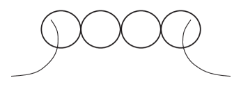
Figure 2. An open rosary of genus three

Note that since $a_{1},\dots,a_{r}$ are tacnodes, we are not able to apply the decomposition formula directly. However, in the proposition below, we shall demonstrate that a similar argument can be used to obtain a systematic analysis of the initial ideal.

Proposition 6.1.

The initial ideal of $R$ with respect to the $\rho$-weighted Lex order satisfies the following decomposition: Let $T_{l}^{d}$ denote the set of degree $d$ monomials in $x_{0},\dots,x_{3l+2}$ (resp. $x_{0},\dots,x_{3r}$) which involve $x_{i}$ and $x_{j}$ for $i<3l-2$ and $j>3l-1$ for $l=1,\dots,r-1$ (resp. $l=r$). We define $x_{l}=x_{0}$ if $l<0$ and $x_{l}=x_{3r}$ if $l>3r$.

1. (degree 2 piece)

   $$(\textup{\bf in}\,I_{R})_{2}\cup\{x_{3l-2}^{2}\}_{l=1}^{r}=\cup_{l=1}^{r+1}\textup{\bf in}\,\left(I_{L_{l}}\cap k[x_{3l-5},\dots,x_{3l-1}]\right)_{2}\cup(\cup_{l=1}^{r}T_{l}^{2})$$

2. (degree 3 piece)

   $$(\textup{\bf in}\,I_{R})_{3}\cup\{x_{3l-2}^{3},x_{3l-2}^{2}x_{3l-1}\}_{l=1}^{r}=\cup_{l=1}^{r+1}\textup{\bf in}\,\left(I_{L_{l}}\cap k[x_{3l-5},\dots,x_{3l-1}]\right)_{3}\cup(\cup_{l=1}^{r}T_{l}^{3})$$

Proof.

The proof follows the idea of Lemma 3.1 closely, but more care needs to be exercised because of the additional overlapping coordinates.

(i)   (degree 2 piece)   Suppose that $x^{\alpha}\in(\textup{\bf in}\,I_{R})_{2}$, then $x^{\alpha}=\textup{\bf in}\,f$ for some homogeneous quadratic $f\in I_{R}$. If $x^{\alpha}$ is not contained in $\cup_{l=1}^{r}T_{l}$, then $x^{\alpha}$ is contained in $k[x_{3l-5},\dots,x_{3l-1}]$ for some $l$. Let $g=f(0,\dots,0,x_{3l-5},\dots,x_{3l-1},0,\dots,0)$. Then $g\in I_{L_{l}}\cap k[x_{3l-5},\dots,x_{3l-1}]$ and therefore, $x^{\alpha}$ is contained in $(\textup{\bf in}\,I_{L_{l}}\cap k[x_{3l-5},\dots,x_{3l-1}])_{2}$. Since $x_{3l-2}^{2}-x_{3l-1}x_{3l}\in I_{L_{l+1}}$, we have $x_{3l-2}^{2}\in\textup{\bf in}\,I_{L_{l}+1}$.

For the other inclusion, suppose that $x^{\alpha}\in(\textup{\bf in}\,I_{L_{l}}\cap k[x_{3l-5},\dots,x_{3l-1}])_{2}$ for some $l=1,2,\dots,r+1$. If $l=1$ or $r+1$, then $x^{\alpha}=x_{0}x_{2}$ or $x_{3r-2}^{2}$ respectively, but we know that $x_{0}x_{2}=\textup{\bf in}\,(x_{0}x_{2}-x_{1}^{2}-x_{2}x_{3})\in\textup{\bf in}\,I_{R}$. Hence $x^{\alpha}$ is contained in the left hand side. If $l=2,3,\dots,r$, then

$$\begin{array}[]{l}I_{L_{l}}=\langle x_{3l-2}^{2}-x_{3l-3}x_{3l-1},x_{3l-3}x_{3l-2}-x_{3l-5}x_{3l-1},x_{3l-5}x_{3l-2}-x_{3l-4}x_{3l-1},\\ x_{3l-3}^{2}-x_{3l-4}x_{3l-1},x_{3l-5}x_{3l-3}-x_{3l-4}x_{3l-2},x_{3l-5}^{2}-x_{3l-4}x_{3l-3}\rangle.\end{array}$$

Let’s denote the generators of $I_{L_{l}}$ by $f_{i}$ for $i=1,2,\dots,6$ in the order shown above.
The initial ideal of $L_{l}$ is

$$\begin{array}[]{lll}\textup{\bf in}\,I_{L_{l}}&=&\langle x_{3l-3}x_{3l-1},x_{3l-4}x_{3l-1},x_{3l-4}x_{3l-2}^{2},x_{3l-5}x_{3l-1},x_{3l-5}x_{3l-2},\\ &&x_{3l-5}x_{3l-3},x_{3l-5}^{2}\rangle\end{array}$$

This shows that $x^{\alpha}$ comes from the initial term of some generator of $I_{L_{l}}$. That is, $x^{\alpha}=\textup{\bf in}\,(f_{i})$ for some $i$. But $f_{i}\in I_{R}$ for $i=2,3,4,5$, it suffices to consider the case $i=1,6$. For the case $i=1$, then $x^{\alpha}=x_{3l-3}x_{3l-1}$ and so $x^{\alpha}\in\textup{\bf in}\,(x_{3l-2}^{2}-x_{3l-3}x_{3l-1}-x_{3l-1}x_{3l})\in\textup{\bf in}\,I_{R}$. For $i=6$, then $x^{\alpha}=x_{3l-5}^{2}$. Obviously, $\cup_{l=1}^{r}T_{l}$ is contained in $\textup{\bf in}\,I_{R}$.

(ii)   (degree 3 piece)   Since $x_{3l-2}^{2}\in\textup{\bf in}\,I_{L_{l+1}}$, $x_{3l-2}^{3}$ and $x_{3l-2}^{2}x_{3l-1}$ are also elements in $I_{L_{l+1}}$. If $x^{\alpha}\in\textup{\bf in}\,I_{R}$ and not in $\cup_{l=1}^{r}T_{l}$, we can easily show that $x^{\alpha}$ is contained in the right hand side by the same proof of the degree 2 case.

For the other inclusion, suppose that $x^{\alpha}$ is a degree three monomial in $\textup{\bf in}\,(I_{L_{l}}\cap k[x_{3l-5},\dots,x_{3l-1}])$ for some $l$. If $l=1$, then $x^{\alpha}=x_{i}(x_{0}x_{2})$ for some $i=0,1,2$. Hence $x^{\alpha}=\textup{\bf in}\,(x_{i}(x_{0}x_{2}-x_{1}^{2}-x_{2}x_{3}))\in\textup{\bf in}\,I_{R}$. If $l=r+1$, then $x^{\alpha}=x_{i}(x_{3r-2})^{2}$ for some $i=3r-2,3r-1,3r$. For $i=3r$, we have $x^{\alpha}=\textup{\bf in}\,(x_{3r}(x_{3r-2}^{2}-x_{3r-1}x_{3r}))\in\textup{\bf in}\,I_{R}$.

Suppose that $l=2,3,\dots,r$, then by using the same notation in degree 2 case, we know that $x^{\alpha}=\textup{\bf in}\,(x_{i}f_{j})$ for $j=1,2,\dots,6$ and $i=3l-5,\dots,3l-1$ except for the case $x^{\alpha}=x_{3l-4}x_{3l-2}^{2}$. If $j=2,3,4,5$, then $x_{i}f_{j}\in I_{R}$ and so $x^{\alpha}\in\textup{\bf in}\,I_{R}$. If $j=1$, then $x^{\alpha}=\textup{\bf in}\,(x_{i}(x_{3l-2}^{2}-x_{3l-3}x_{3l-1}-x_{3l-1}x_{3l}))\in\textup{\bf in}\,I_{R}$. Hence it remains to consider the case $j=6$ and $x^{\alpha}=x_{3l-4}x_{3l-2}^{2}$.

For the case $j=6$, suppose that $x^{\alpha}=\textup{\bf in}\,(x_{i}f_{6})=x_{i}x_{3l-5}^{2}$. For $i=3l-5,3l-4$, there is nothing to prove. If $i>3l-4$, then $x^{\alpha}=\textup{\bf in}\,(x_{3l-5}f_{j})$ for $j=2,3,5$. Hence $x^{\alpha}\in\textup{\bf in}\,I_{R}$ since $f_{j}\in I_{R}$ where $j=2,3,5$. For the case $x^{\alpha}=x_{3l-4}x_{3l-2}^{2}$, $x^{\alpha}=x_{3l-4}x_{3l-2}^{2}=\textup{\bf in}\,\{x_{3l-4}(f_{1}-x_{3l-1}x_{3l})+x_{3l-3}(f_{4})\}\in\textup{\bf in}\,I_{R}$ since $f_{1}-x_{3l-1}x_{3l}$ and $f_{4}$ are elements in $I_{R}$. Finally, $\cup_{l=1}^{r}T_{l}$ is contained in $\textup{\bf in}\,I_{R}$. This completes the proof. ∎

By using the above proposition, we can compute inductively the sum of $\rho$-weights of degree 2 and 3 monomials in the initial ideal of $I_{R}$. Let $w_{i}(r)$ be the sum $\underset{x^{\alpha}\in\textup{\bf in}\,(I_{R})_{i}}{\Sigma}wt_{\rho}(x^{\alpha})$ for $i=2,3$ where $R$ is the open rosary of length $r+1$. Then

$$w_{2}(r)=\left\{\begin{array}[]{ll}w_{2}(r-2)+(72r-110)&\textrm{for odd $r>1$}\\ w_{2}(r-2)+(72r-92)&\textrm{for even $r>2$}\\ \end{array}\right.$$

For the degree 3 case,

$$w_{3}(r)=\left\{\begin{array}[]{ll}w_{3}(r-2)+(162r^{2}-162r-57)&\textrm{for odd $r>1$}\\ w_{3}(r-2)+(162r^{2}-108r-66)&\textrm{for even $r>2$}\\ \end{array}\right.$$

Since $w_{2}(1)=6,w_{2}(2)=52,w_{3}(1)=34,w_{3}(2)=366$, we can easily compute the $w_{i}(r)$ as follows.

$$w_{2}(r)=\left\{\begin{array}[]{ll}18r^{2}-19r+7&\textrm{for odd $r$}\\ 18r^{2}-10r&\textrm{for even $r$}\\ \end{array}\right.$$

and

$$w_{3}(r)=\left\{\begin{array}[]{ll}27r^{3}+\frac{81}{2}r^{2}-\frac{111}{2}r+22&\textrm{for odd $r$}\\ 27r^{3}+54r^{2}-33r&\textrm{for even $r$}\\ \end{array}\right.$$

which is consistent with the results in [HH13, Section 8.1].

References

- [AFS10] Jarod Alper, Maksym Fedorchuk, and David Ishii Smyth. Singularities with -action and the log minimal model program for , 2010. arXiv:1010.3751v1 [math.AG].
- [BM88] David Bayer and Ian Morrison. Standard bases and geometric invariant theory. I. Initial ideals and state polytopes. J. Symbolic Comput., 6(2-3):209–217, 1988. Computational aspects of commutative algebra.
- [GS] Daniel R. Grayson and Michael E. Stillman. Macaulay2, a software system for research in algebraic geometry. Available at http://www.math.uiuc.edu/Macaulay2/.
- [HH13] Brendan Hassett and Donghoon Hyeon. Log minimal model program for the moduli space of curves: the first flip. Ann. of Math. (2), 177(3):911–968, 2013.
- [HHL10] Brendan Hassett, Donghoon Hyeon, and Yongnam Lee. Stability computation via Gröbner basis. J. Korean Math. Soc., 47(1):41–62, 2010.
- [HM10] Donghoon Hyeon and Ian Morrison. Stability of tails and 4-canonical models. Math. Res. Lett., 17(4):721–729, 2010.
- [Kem78] George R. Kempf. Instability in invariant theory. Ann. of Math. (2), 108(2):299–316, 1978.
- [MS11] Ian Morrison and David Swinarski. Gröbner techniques for low-degree Hilbert stability. Exp. Math., 20(1):34–56, 2011.
- [Mum65] D. Mumford. Geometric invariant theory. Ergebnisse der Mathematik und ihrer Grenzgebiete, Neue Folge, Band 34. Springer-Verlag, Berlin, 1965.
- [Sch91] David Schubert. A new compactification of the moduli space of curves. Compositio Math., 78(3):297–313, 1991.
- [Stu96] Bernd Sturmfels. Gröbner bases and convex polytopes, volume 8 of University Lecture Series. American Mathematical Society, Providence, RI, 1996.